The Character of $\mathrm{Z}$-pole Data Constraints on
Standard Model Parameters

Abstract

Despite the impressive precision of the $\mathrm{Z}$-pole measurements made with the e+ e- colliders at CERN (LEP) and SLAC (SLC), the allowed region for the principle Standard Model parameters responsible for radiative corrections ($m_{\mathrm{H}}$, $m_{\mathrm{t}}$, and $\alpha(m_{\mathrm{Z}}^{2})$) is still large enough to encompass significant non-linearities. The nature of the experimental constraints therefore depends in an interesting way on the “accidental” relationships among the various measurements. In particular, the fact that the $\mathrm{Z}$-pole measurements favor values of $m_{\mathrm{H}}$ excluded by direct searches leads us to examine the effects of external Higgsstrahlung, a process ignored by the usual precision electroweak calculations.

I Introduction

The precise measurements of $\mathrm{Z}$ resonance properties made by the four collaborations at the CERN $\mathrm{e}^{+}\mathrm{e}^{-}$ collider LEP and by the SLAC Large Detector (SLD) at the SLC have confirmed all relevant predictions of the Standard Model, and established a strong experimental basis for the mechanism of symmetry breaking in the electroweak sector. The two fundamental equations of electroweak unification,

$$\sin^{2}\theta_{\mathrm{W}} = \frac{\pi\alpha}{\sqrt{2}m_{\mathrm{W}}^{2}G_{\mathrm{F}}},$$ (1)

$$\cos^{2}\theta_{\mathrm{W}} = \frac{m_{\mathrm{W}}^{2}}{m_{\mathrm{Z}}^{2}\rho_{0}},$$ (2)

establish the relations between the strengths of the electromagnetic and weak couplings, and the mass ratio of the neutral and charged heavy vector bosons. Here $G_{\mathrm{F}}$ is the Fermi constant determined in muon decay, $\alpha$ is the electromagnetic fine-structure constant, $m_{\mathrm{W}}$ and $m_{\mathrm{Z}}$ are the W and $\mathrm{Z}$ boson masses, and $\theta_{\mathrm{W}}$ is the electroweak mixing angle. The $\rho_{0}$ parameterRoss and Veltman (1975) is determined by the Higgs structure of the theory; in the Minimal Standard Model which we consider here, $\rho_{0}$ is unity.

$G_{\mathrm{F}}$, $m_{\mathrm{Z}}$, and $\alpha(m_{\mathrm{Z}}^{2})$ are known with relative precisions of (1, 2 and 40)$\times 10^{-5}$. This allows the radiative corrections to Equations 1 and 2 to be investigated in considerable detail. These radiative corrections depend principally on the masses of the top quark, $m_{\mathrm{t}}$, and the Higgs boson, $m_{\mathrm{H}}$. One of the great strengths of the $\mathrm{Z}$-pole data is that the measurements of the partial widths and charge asymmetries allow the effects of the Higgs boson and the top quark to be separated to a remarkable extent. The character of this separation is the primary topic of this paper.

Since the top quark has been observed directly, the agreement between the directly measured mass and its indirect measurement derived through the radiative corrections provides compelling evidence that the theoretical and experimental understanding of the $\mathrm{Z}$-pole measurements rests upon firm ground. The much smaller effects due to $m_{\mathrm{H}}$ then provide essentially the only experimental knowledge we have concerning this elusive particle, apart from the fact that it has so far escaped direct observation.

The broad range of $m_{\mathrm{H}}$ still consistent with the measurements provides sufficient room for non-linear effects to become important. Such non-linearities mean that the gaussian error hypothesis, which is implicit in the $\chi^{2}$ fits used to determine the error contours of the Standard Model parameters, approximates the true errors only imperfectly. The actual errors and even the shape of the measurement constraints depend significantly on the working point of the fit in the multi-dimensional space describing the range accessible to the parameters. The character of the $m_{\mathrm{t}}$, $m_{\mathrm{H}}$ separation therefore depends in an interesting manner on the “accidental” relations between the various measurements. Variations on the scale of the expected measurement uncertainties can, in some cases, lead to disproportionate shifts in the error contours. In other cases, the specific manner in which a measurement happens to lie within its band of uncertainty results in unanticipated stability. Some understanding of these subtle effects is necessary for a full appreciation of the measurements.

Since we are interested in describing how our knowledge is augmented by each individual measurement as well as sets of measurements in combination, we are led naturally to consider hypothetical situations which explicitly violate constraints lying beyond the set of measurements being considered at any particular moment. Chief among the constraints we often ignore is the experimental lower limit on $m_{\mathrm{H}}$ provided by the direct searches LEP (2003). A related complication in the analysis arises from what may be an historical accident. Due to the early and continued non-observation of the Higgs boson at LEP, the two most precise electroweak programs, ZFITTER Bardin et al. (1989, 1990, 1991a, 1991b, 1992, 2001) and TOPAZ0 Montagna et al. (1993a, b); Montagna et al. (1996, 1999), do not include the effects of external Higgs boson emission from the $\mathrm{Z}$ propagator. Since the $\mathrm{Z}$-pole measurements in fact favor a low-mass Higgs boson, we are led to consider the effects of such Higgsstrahlung in order to provide a self-consistent picture of what these measurements alone tell us about the Standard Model.

II Radiative Corrections

The largest radiative correction affecting the basic electroweak relations presented in the previous section is due to the running of the electromagnetic coupling constant in Equation 1. This running is due to the presence of fermion loops in the photon propagator, and is usually parametrized as:

$$\alpha(s)=\frac{\alpha(0)}{1-\Delta\alpha(s)}.$$ (3)

Near the $\mathrm{Z}$-pole, leptons, the top quark, and the five light quarks contribute to $\Delta\alpha(s)$:

$$\Delta\alpha(s)=\Delta\alpha_{\mathrm{e\mu\tau}}(s)+\Delta\alpha_{\mathrm{top}}(s)+\Delta\alpha_{\mathrm{had}}^{(5)}(s).$$ (4)

The $\mathrm{Z}$-pole data itself gives no useful experimental constraints on $\Delta\alpha(s)$. The first two terms of Equation 4 can be precisely calculated, but $\Delta\alpha_{\mathrm{had}}^{(5)}(s)$ is best determined by analyzing the measured rate of $\mathrm{e}^{+}\mathrm{e}^{-}$ annihilation to hadrons using a dispersion relation Burkhardt and Pietrzyk (2001), where low-energy data dominates the resulting uncertainty. At LEP/SLC energies, $\alpha$ is increased from the Thompson limit of $1/137.036$ to $1/128.945$, corresponding to $\Delta\alpha^{(5)}_{\mathrm{had}}(m_{\mathrm{Z}}^{2})=0.02761\pm 0.00036$ Burkhardt and Pietrzyk (2001).

Combining Equations 1 and 2, and including radiative corrections yields:

$$\cos^{2}\theta_{\mathrm{W}}\sin^{2}\theta_{\mathrm{W}} = \frac{\pi\alpha(0)}{\sqrt{2}m_{\mathrm{Z}}^{2}G_{\mathrm{F}}}\frac{1}{1-(\Delta\alpha+\Delta{r}_{\mathrm{w}})},$$ (5)

where $\Delta{r}_{\mathrm{w}}$ represents further weak corrections. Equation 5 directly links $\Delta\alpha$ and $\Delta{r}_{\mathrm{w}}$ to the value of $\theta_{\mathrm{W}}$, and hence to $m_{\mathrm{W}}$ via Equation 2.

Radiative corrections also affect the couplings of the $\mathrm{Z}$ to fermions. The bulk of these correctionsVeltman (1977) can be absorbed into an over-all scale factor for the couplings, $\rho_{\mathrm{f}}$, and a scale factor, $\kappa_{\mathrm{f}}$, for the electroweak mixing angle, resulting in “effective” quantities:

$$\rho_{\mathrm{f}} = 1+\Delta\rho_{\mathrm{se}}+\Delta\rho_{\mathrm{f}}$$ (6)

$$\kappa_{\mathrm{f}} = 1+\Delta\kappa_{\mathrm{se}}+\Delta\kappa_{\mathrm{f}}$$ (7)

$$\sin^{2}\theta_{\mathrm{eff}}^{{\rm f}} = \kappa_{\mathrm{f}}\sin^{2}\theta_{\mathrm{W}}$$ (8)

$$g_{\mathrm{Vf}} = \sqrt{\rho_{\mathrm{f}}}(T_{f}^{3}-2Q_{f}\sin^{2}\theta_{\mathrm{eff}}^{{\rm f}})$$ (9)

$$g_{\mathrm{Af}} = \sqrt{\rho_{\mathrm{f}}}T_{f}^{3}.$$ (10)

Here $T_{f}^{3}$ is the third component of weak isospin, $Q_{f}$ is the charge, $\theta_{\mathrm{eff}}^{{\rm f}}$ is the effective electroweak mixing angle, and $g_{\mathrm{Vf}}$ and $g_{\mathrm{Af}}$ are the effective vector and axial-vector couplings for the fermion species f. The quantities $\Delta\rho_{\mathrm{se}}$ and $\Delta\kappa_{\mathrm{se}}$ are universal corrections arising from the propagator self-energies, while $\Delta\rho_{\mathrm{f}}$ and $\Delta\kappa_{\mathrm{f}}$ are flavor-specific vertex corrections. The effective couplings $g_{\mathrm{Vf}}$ and $g_{\mathrm{Af}}$ are purely real, and describe that part of the $\mathrm{Z}$ interaction which can be treated as a resonance in the Improved Born Approximation. The remaining, complex parts, termed “remnants”, generate effects which are small compared to the experimental errors, but are nevertheless respected when determining $g_{\mathrm{Vf}}$ and $g_{\mathrm{Af}}$ from the data (see, for example Abbiendi et al. (2001)).

The $\mathrm{Z}$ partial width to each fermion species, $\Gamma_{\mathrm{f\bar{f}}}$, is proportional to $\rho_{\mathrm{f}}$, while $\sin^{2}\theta_{\mathrm{eff}}^{\mathrm{lept}}$, measured through the asymmetries, is proportional to $\kappa_{\mathrm{f}}$. Calculations at one-loop order illustrate the essential $m_{\mathrm{t}}$ and $m_{\mathrm{H}}$ dependenciesBurgers and Jegerlehner (1989), which are quadratic in $m_{\mathrm{t}}$ and logarithmic in $m_{\mathrm{H}}$. The dependence of $\Delta\kappa_{\mathrm{se}}$ remains the same over the entire range of $m_{\mathrm{H}}$:

$$\Delta\kappa_{\mathrm{se}}= \frac{3G_{\mathrm{F}}m_{\mathrm{W}}^{2}}{8\sqrt{2}\pi^{2}}\frac{m_{\mathrm{t}}^{2}}{m_{\mathrm{W}}^{2}}\frac{\cos^{2}\theta_{\mathrm{W}}}{\sin^{2}\theta_{\mathrm{W}}}-$$ (11)

$$\frac{10}{3}\frac{G_{\mathrm{F}}m_{\mathrm{W}}^{2}}{8\sqrt{2}\pi^{2}}\left(\ln\frac{m_{\mathrm{H}}^{2}}{m_{\mathrm{W}}^{2}}-\frac{5}{6}\right)+\cdots.$$

For $\Delta\rho_{\mathrm{se}}$, the sign of the dependence on $ln(m_{\mathrm{H}})$ is negative for $m_{\mathrm{H}}\gg m_{\mathrm{W}}$:

$$\Delta\rho_{\mathrm{se}}= \frac{3G_{\mathrm{F}}m_{\mathrm{W}}^{2}}{8\sqrt{2}\pi^{2}}\frac{m_{\mathrm{t}}^{2}}{m_{\mathrm{W}}^{2}}-$$ (12)

$$\frac{3G_{\mathrm{F}}m_{\mathrm{W}}^{2}}{8\sqrt{2}\pi^{2}}\frac{\sin^{2}\theta_{\mathrm{W}}}{\cos^{2}\theta_{\mathrm{W}}}\left(\ln\frac{m_{\mathrm{H}}^{2}}{m_{\mathrm{W}}^{2}}-\frac{5}{6}\right)+\cdots$$

and positive for $m_{\mathrm{H}}\ll m_{\mathrm{W}}$:

$$\Delta\rho_{\mathrm{se}}= \frac{3G_{\mathrm{F}}m_{\mathrm{W}}^{2}}{8\sqrt{2}\pi^{2}}\frac{m_{\mathrm{t}}^{2}}{m_{\mathrm{W}}^{2}}+$$ (13)

$$\frac{G_{\mathrm{F}}m_{\mathrm{Z}}^{2}}{4\sqrt{2}\pi^{2}}\ln\frac{m_{\mathrm{H}}^{2}}{m_{\mathrm{Z}}^{2}}-\frac{7G_{\mathrm{F}}m_{\mathrm{H}}m_{\mathrm{Z}}}{8\sqrt{2}\pi}\cdots.$$

Equation 8 shows that $\sin^{2}\theta_{\mathrm{eff}}^{\mathrm{lept}}$ receives radiative corrections from both $\Delta{r}_{\mathrm{w}}$, through $\sin^{2}\theta_{\mathrm{W}}$, and from $\Delta\kappa_{\mathrm{se}}$ directly. These corrections act along the same axis in the $m_{\mathrm{t}}\,vs\,\ln(m_{\mathrm{H}})$ plane, but in opposite senses due to the near equality, in single-loop approximation:

$$\Delta\kappa_{\mathrm{se}} = -\Delta{r}_{\mathrm{w}}+\cdots.$$ (14)

In the $m_{\mathrm{t}}\,vs\,\ln(m_{\mathrm{H}})$ plane lines of constant $\Delta\kappa_{\mathrm{se}}$ and $\Delta{r}_{\mathrm{w}}$, and hence $m_{\mathrm{W}}$ and $\sin^{2}\theta_{\mathrm{eff}}^{\mathrm{lept}}$ are therefore all approximately parallel. When moving along such lines, then, changes in the radiative effects of the top quark and the Higgs boson are seen to cancel. It is only through violations of this approximation that measurements of $m_{\mathrm{W}}$ and $\sin^{2}\theta_{\mathrm{eff}}^{\mathrm{lept}}$ have any power to separate the effects of $m_{\mathrm{t}}$ and $m_{\mathrm{H}}$.

The fact that $\Delta{r}_{\mathrm{w}}$ and $\Delta\kappa_{\mathrm{se}}$ oppose each other in Equation 8 reduces the sensitivity of $\sin^{2}\theta_{\mathrm{eff}}^{\mathrm{lept}}$ to the corrections. The effect of $\Delta{r}_{\mathrm{w}}$ is larger, so that changes in $\sin^{2}\theta_{\mathrm{eff}}^{\mathrm{lept}}$ are of the same sign as those in $\sin^{2}\theta_{\mathrm{W}}$, but are a factor of $\sin^{2}\theta_{\mathrm{W}}$/$\cos^{2}\theta_{\mathrm{W}}$ smaller in magnitude Jegerlehner (1991a), which is about $0.3$.

Since $\sin^{2}\theta_{\mathrm{W}}$ is present in the dominant, $m_{\mathrm{t}}$, term of Equation 11, but absent in the corresponding terms of Equations 12 and 13, the effects of $\Delta\alpha^{(5)}_{\mathrm{had}}(m_{\mathrm{Z}}^{2})$ are felt in $\Delta\kappa_{\mathrm{se}}$, but $\Delta\rho_{\mathrm{se}}$ is well isolated. The uncertainty in $\Delta\alpha^{(5)}_{\mathrm{had}}(m_{\mathrm{Z}}^{2})$ therefore dilutes the inherent precision of the $\sin^{2}\theta_{\mathrm{eff}}^{\mathrm{lept}}$ measurements, but not those of the partial widths.

Similarly, the weak effects of $\Delta{r}_{\mathrm{w}}$ are felt undiluted in $m_{\mathrm{W}}$, so that the relative effect of $\Delta\alpha$ is much smaller there than it is for $\sin^{2}\theta_{\mathrm{eff}}^{\mathrm{lept}}$, where about $0.7$ of the weak corrections are canceled through $\Delta\kappa_{\mathrm{se}}$.

The flavour dependence of the radiative corrections is very small for all fermions, except for the b quark, where vertex corrections are significant due to the large mass splitting between the bottom and top quarks Jegerlehner (1991b), resulting in:

$$\Delta\rho_{\mathrm{b}} = -\frac{G_{\mathrm{F}}m_{\mathrm{t}}^{2}}{2\sqrt{2}\pi^{2}}+\cdots.$$ (15)

Notice that $\Delta\rho_{\mathrm{b}}$ has no Higgs dependence, making the quantity $R_{\mathrm{b}}^{0}=\Gamma_{\mathrm{b\overline{b}}}/\Gamma_{\mathrm{had}}$ a straight-forward indicator of $m_{\mathrm{t}}$, since the $m_{\mathrm{H}}$ dependences entering through $\Delta\rho_{\mathrm{se}}$ cancel in numerator and denominator.

The partial Z decay widths contain final state radiative corrections and add up straightforwardly to yield the total width of the $\mathrm{Z}$ boson Bardin et al. (1999):

$$\Gamma_{\mathrm{f\bar{f}}}= N_{c}^{\rm f}\frac{G_{\mathrm{F}}m_{\mathrm{Z}}^{3}}{6\sqrt{2}\pi}\left(|{\cal G}_{\mathrm{Af}}|^{2}R_{\mathrm{Af}}+|{\cal G}_{\mathrm{Vf}}|^{2}R_{\mathrm{Vf}}\right)$$ (16)

$$+\Delta_{\rm ew/QCD}.$$

Here the complex effective couplings, ${\cal G}_{\mathrm{Vf}}$ and ${\cal G}_{\mathrm{Af}}$ differ only by small imaginary parts from the real effective couplings defined in Equations 9 and 10. The radiator factors $R_{\mathrm{Vf}}$ and $R_{\mathrm{Af}}$ take into account final state QED and QCD Chetyrkin et al. (1995) corrections including pair production; $\Delta_{\rm ew/QCD}$ accounts for small contributions from non-factorizable electroweak/QCD corrections.

Although the discussion of electroweak corrections presented above (Equations 11–15) is at the single loop level, serious quantitative calculations implemented in programs such as ZFITTER and TOPAZ0 include terms of higher order. These programs can not only calculate the effective couplings as a function of the free Standard Model parameters, but can also relate these couplings to observables such as cross sections and partial widths. The simple single-loop expressions are nevertheless useful in understanding the results of the elaborate, very precise calculations used in deriving our quantitative results.

III $\mathrm{Z}$-pole Constraints on $m_{\mathrm{t}}$ and $m_{\mathrm{H}}$

As $\mathrm{Z}$-pole input data we consider the set listed in Table 16.1 of reference Gro , which consists of $\Delta\alpha^{(5)}_{\mathrm{had}}(m_{\mathrm{Z}}^{2})$, plus the 14 $\mathrm{Z}$-pole measurements: $m_{\mathrm{Z}}$, $\Gamma_{\mathrm{Z}}$, $\sigma_{\mathrm{h}}^{0}$, $R^{0}_{\ell}$, $A^{0,\,\ell}_{\mathrm{FB}}$, ${\cal A}_{\ell}~{}(P_{\tau})$, $\sin^{2}\theta_{\mathrm{eff}}^{\mathrm{lept}}$(${\langle Q_{\mathrm{FB}}\rangle}$), ${\cal A}_{\ell}$ (SLD), $R_{\mathrm{b}}^{0}{}$, $R_{\mathrm{c}}^{0}{}$, $A^{0,\,{\mathrm{b}}}_{\mathrm{FB}}{}$, $A^{0,\,{\mathrm{c}}}_{\mathrm{FB}}{}$, ${\cal A}_{\mathrm{b}}$, and ${\cal A}_{\mathrm{c}}$, including their error correlations. We perform Standard Model fits to this data, using ZFITTER 6.36 to predict the observables as a function of the five free parameters: $\Delta\alpha^{(5)}_{\mathrm{had}}(m_{\mathrm{Z}}^{2})$, $m_{\mathrm{Z}}$, $\alpha_{\mathrm{S}}$, $m_{\mathrm{t}}$ and $m_{\mathrm{H}}$.

To illustrate the constraints imposed by these measurements, it is useful to group them according to their functional roles. Two quantities, $\Delta\alpha^{(5)}_{\mathrm{had}}(m_{\mathrm{Z}}^{2})$ and $m_{\mathrm{Z}}$, appear as both input data and fit parameters. The electromagnetic coupling, parametrized through $\Delta\alpha^{(5)}_{\mathrm{had}}(m_{\mathrm{Z}}^{2})$, is determined externally  Burkhardt and Pietrzyk (2001), and passes through the $\mathrm{Z}$-pole fit as an inert ingredient. Similarly, $m_{\mathrm{Z}}$ is determined with such precision that it is incapable of being pulled by its dynamic relation to other quantities. Both might just as well have been treated as external constants, like $G_{\mathrm{F}}$. The b- and c-quark asymmetry parameters, ${\cal A}_{\mathrm{b}}$, and ${\cal A}_{\mathrm{c}}$ are also inert in the fit, since they have essentially no dependence on the Standard Model parameters.

The three measurements $\Gamma_{\mathrm{Z}}$, $\sigma_{\mathrm{h}}^{0}$ and $R^{0}_{\ell}$ are equivalent to the more meaningful, but more correlated quantities $\Gamma_{\ell\ell}$, $\Gamma_{\mathrm{had}}$ and $\Gamma_{\mathrm{inv}}/\Gamma_{\ell\ell}$. Of these, the latter is insensitive to variations in the Standard Model Parameters, and serves to measure the number of light neutrino generations. The strong coupling constant, $\alpha_{\mathrm{S}}$, is determined by its effect on the hadronic width, $\Gamma_{\mathrm{had}}$, leaving $\Gamma_{\ell\ell}$ as the key quantity in constraining $\Delta\rho_{\mathrm{se}}$. The small size of $g_{\mathrm{V\ell}}$ compared to $g_{\mathrm{A\ell}}$ (see Equation 9) makes $\Gamma_{\ell\ell}$ essentially independent of $\sin^{2}\theta_{\mathrm{eff}}^{\mathrm{lept}}$.

As already discussed in connection with Equation 15, $R_{\mathrm{b}}^{0}$ serves as a direct indicator of $m_{\mathrm{t}}$. The role of $R_{\mathrm{c}}^{0}$ is diffuse and non-critical.

The six remaining measurements, $A^{0,\,\ell}_{\mathrm{FB}}$, ${\cal A}_{\ell}~{}(P_{\tau})$, $\sin^{2}\theta_{\mathrm{eff}}^{\mathrm{lept}}$(${\langle Q_{\mathrm{FB}}\rangle}$), ${\cal A}_{\ell}$ (SLD), $A^{0,\,{\mathrm{b}}}_{\mathrm{FB}}{}$, and $A^{0,\,{\mathrm{c}}}_{\mathrm{FB}}{}$ serve to determine the single quantity $\sin^{2}\theta_{\mathrm{eff}}^{\mathrm{lept}}$. Although there is a disturbing lack of consistency between the values of $\sin^{2}\theta_{\mathrm{eff}}^{\mathrm{lept}}$ derived from the two most precise measurements, ${\cal A}_{\ell}$ (SLD) and $A^{0,\,{\mathrm{b}}}_{\mathrm{FB}}{}$, the discrepancy ($\approx 2.9\sigma$) between them appears to elude explanation. Within the Standard Model all six of these measurements, and particularly the two most precise, appear to be valid and well-defined measurements of $\sin^{2}\theta_{\mathrm{eff}}^{\mathrm{lept}}$.

Both measurements claim to be dominated by statistical uncertainties. The measurements Gro of $A^{0,\,{\mathrm{b}}}_{\mathrm{FB}}{}$ are complex, but the level of agreement between the independent analyses of the four LEP Collaborations is excellent. Common QCD corrections play a role, but are believed to be well understood. The SLD measurement Abe et al. (2001) of ${\cal A}_{\ell}$ through $A_{\mathrm{LR}}$, the asymmetry between the interaction rate for right- and left-handed electron beam polarizations, is both simple and elegant. The least implausible source of systematic error, in the measurement of the beam polarization, is believed to be small and well-controlled.

Here we investigate the consequences of excluding either ${\cal A}_{\ell}$ (SLD) or $A^{0,\,{\mathrm{b}}}_{\mathrm{FB}}{}$ from the fit, but we make no attempt to choose between them. Either exclusion option restores acceptable consistency to the set of $\sin^{2}\theta_{\mathrm{eff}}^{\mathrm{lept}}$ measurements, but obviously introduces a bias.

The constraints on $m_{\mathrm{t}}$ and $m_{\mathrm{H}}$ imposed by the 14 $\mathrm{Z}$-pole measurements can therefore be almost completely expressed in terms of three quantities:

$\Gamma_{\ell\ell}$ - related directly to $\Delta\rho_{\mathrm{se}}$

$\sin^{2}\theta_{\mathrm{eff}}^{\mathrm{lept}}$ - related directly to $\Delta\kappa_{\mathrm{se}}$, and

$R_{\mathrm{b}}^{0}$ - related directly to $m_{\mathrm{t}}$.

III.1 $\mathrm{Z}$-pole Data Constraints Alone

How these components of the Z-pole data constrain $m_{\mathrm{t}}$ and $m_{\mathrm{H}}$ can be clearly illustrated on a plot of $m_{\mathrm{t}}\,vs\,\log_{10}(m_{\mathrm{H}}/\mathrm{GeV})$, as shown in Figure 1.

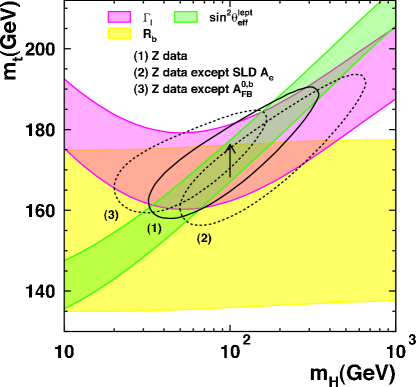
Figure 1: $m_{\mathrm{t}}$ and $m_{\mathrm{H}}$ constraints from the Z-pole measurements. Each band gives the $\pm 1\sigma$ constraint from the indicated measurement. The arrow indicates the additional variation in $\sin^{2}\theta_{\mathrm{eff}}^{\mathrm{lept}}$ due to a $\pm 1\sigma$ uncertainty in $\Delta\alpha^{(5)}_{\mathrm{had}}(m_{\mathrm{Z}}^{2})$. The ellipses give the 68% CL fit contours for the indicated data.

Shown here are the usual 68% CL error contours, plotted by finding the curve in the $m_{\mathrm{t}}\,vs\,\log_{10}(m_{\mathrm{H}}/\mathrm{GeV})$ plane where the $\chi^{2}$ of the fit exceeds its minimum by 2.28. For projections in a single parameter, 68% CL corresponds to $1.51\sigma$. Also plotted are measurement constraint bands, which show the contribution of each measurement. These are plotted by finding the curves in the $m_{\mathrm{t}}\,vs\,\log_{10}(m_{\mathrm{H}}/\mathrm{GeV})$ plane where the predicted value of the measured quantity equals the central value of the measurement $\pm 1\sigma$. Note that since each of these bands indicate the constraint imposed by a fixed measurement, it exhibits exactly the inverse parameter dependence compared to the Standard Model prediction for the measured quantity.

The diagonal band in Figure 1 indicates the $\pm 1\sigma$ constraint from the $\sin^{2}\theta_{\mathrm{eff}}^{\mathrm{lept}}$ measurements. Higher-order electroweak corrections do not significantly affect the linear relationship expected from the lowest-order terms, and the slope of this band is approximated by the ratio of the coefficients of $m_{\mathrm{t}}^{2}$ and $ln(m_{\mathrm{H}})$ in the expression for $\Delta\kappa_{\mathrm{se}}$:

$$\left.\frac{dm_{\mathrm{t}}}{dln(m_{\mathrm{H}})}\right|_{\kappa_{\mathrm{se}}} = \frac{10}{9}\frac{m_{\mathrm{Z}}^{2}\sin^{2}\theta_{\mathrm{W}}}{m_{\mathrm{t}}}.$$ (17)

The banana-shaped band in Figure 1 shows the $\pm 1\sigma$ constraint from the $\Gamma_{\ell\ell}$ measurement. The slope of this band at large $\log_{10}(m_{\mathrm{H}}/\mathrm{GeV})$ agrees reasonably with the linear relation expected from the ratio of coefficients in the lowest-order expression for $\Delta\rho_{\mathrm{se}}$ in this region:

$$\left.\frac{dm_{\mathrm{t}}}{dln(m_{\mathrm{H}})}\right|_{\rho_{\mathrm{se}}} = \frac{m_{\mathrm{Z}}^{2}}{m_{\mathrm{t}}}\sin^{2}\theta_{\mathrm{W}}.$$ (18)

Also at low $\log_{10}(m_{\mathrm{H}}/\mathrm{GeV})$ the slope, now negative, agrees with the lowest-order expression given in Equation 13:

$$\left.\frac{dm_{\mathrm{t}}}{dln(m_{\mathrm{H}})}\right|_{\rho_{\mathrm{se}}} = -\frac{2m_{\mathrm{Z}}^{2}}{3m_{\mathrm{t}}}.$$ (19)

Due to the fact that $R_{\mathrm{b}}^{0}$ is controlled by vertex corrections determined by the $t-b$ mass-splitting, its measurement provides a constraint on $m_{\mathrm{t}}$ almost independent of $\log_{10}(m_{\mathrm{H}}/\mathrm{GeV})$, as shown by the broad horizontal band in Figure 1 (also $\pm 1\sigma$).

The central ellipse in Figure 1 shows the 68% CL contour for the Standard Model fit to all Z-pole measurements. The dominant role played by $\sin^{2}\theta_{\mathrm{eff}}^{\mathrm{lept}}$ in determining the minor axis is evident, and the turn-over of the $\Gamma_{\ell\ell}$ banana provides the lower bound of the major axis. The $R_{\mathrm{b}}^{0}$ measurement provides the upper bound. If the $R_{\mathrm{b}}^{0}$ constraint is removed, the fit in fact no longer yields a 68% CL upper limit for $m_{\mathrm{H}}$ or $m_{\mathrm{t}}$.

The other two ellipses in Figure 1 show similar fit contours when either the $A_{\mathrm{LR}}$ or the $A^{0,\,{\mathrm{b}}}_{\mathrm{FB}}$ measurements are excluded from the fit. The noticeable shrinkage of the major axis in the case when the $A^{0,\,{\mathrm{b}}}_{\mathrm{FB}}$ measurement is dropped is due to the fact that the $\sin^{2}\theta_{\mathrm{eff}}^{\mathrm{lept}}$ constraint then begins to move around the corner of the $\Gamma_{\ell\ell}$ banana. If the $\sin^{2}\theta_{\mathrm{eff}}^{\mathrm{lept}}$ measurement moved even lower in $m_{\mathrm{H}}$, the $\sin^{2}\theta_{\mathrm{eff}}^{\mathrm{lept}}$ and $\Gamma_{\ell\ell}$ constraints would become almost perpendicular, eliminating the usual $m_{\mathrm{t}}-\log_{10}(m_{\mathrm{H}}/\mathrm{GeV})$ error correlation.

The agreement of the indirect measurement of $m_{\mathrm{t}}$ from the Z-pole measurements alone with the direct measurement made in $\mathrm{p\overline{p}}$ collisions Hagiwara et al. (2002) ($m_{\mathrm{t}}=174.3\pm 5.1$ GeV) is an important experimental confirmation of the validity of electroweak corrections. The remarkable stability of the indirect measurement’s central value under shifts in $\sin^{2}\theta_{\mathrm{eff}}^{\mathrm{lept}}$ can be seen to result from a complex interplay between the relatively weak constraint from $R_{\mathrm{b}}^{0}$, which happens to lie low, and the exact relation between the $\sin^{2}\theta_{\mathrm{eff}}^{\mathrm{lept}}$ measurement band and the position of the $\Gamma_{\ell\ell}$ corner.

The arrow in Figure 1 shows how the $\sin^{2}\theta_{\mathrm{eff}}^{\mathrm{lept}}$ measurement band would shift under a $\pm 1\sigma$ change in the $\Delta\alpha^{(5)}_{\mathrm{had}}(m_{\mathrm{Z}}^{2})$ determination. Only the $\sin^{2}\theta_{\mathrm{eff}}^{\mathrm{lept}}$ measurement is significantly sensitive to $\Delta\alpha^{(5)}_{\mathrm{had}}(m_{\mathrm{Z}}^{2})$ on the scale of the current errors, making the effective width of the $\sin^{2}\theta_{\mathrm{eff}}^{\mathrm{lept}}$ measurement band in the $m_{\mathrm{t}}\,vs\,m_{\mathrm{H}}$ plane about 50% wider than the band shown, which corresponds to $\Delta\alpha^{(5)}_{\mathrm{had}}(m_{\mathrm{Z}}^{2})$ fixed at its central value.

The effect of applying the constraint of the direct $m_{\mathrm{t}}$ measurement Hagiwara et al. (2002) can easily be visualized by imagining a horizontal band at $m_{\mathrm{t}}=174.3\pm 5.1$ GeV. Notice that at the operating point of the Z-pole fit, the direct $m_{\mathrm{t}}$ measurement essentially surplants not only $R_{\mathrm{b}}^{0}$, but also the constraints provided by $\Gamma_{\ell\ell}$.

It is perhaps interesting to remark on the fact that all measurements are compatible with the broad $\Gamma_{\ell\ell}$ extremum in $\log_{10}(m_{\mathrm{H}}/\mathrm{GeV})$. Only the failure to find direct production of the Higgs boson at LEP II indicates nature’s choice to lie on the $\Gamma_{\ell\ell}$ upper branch.

III.2 Additional Constraints from $m_{\mathrm{W}}$

Direct measurements of $m_{\mathrm{W}}$ also provide important constraints on the Standard Model parameters through the electroweak corrections $\Delta{r}_{\mathrm{w}}$. The high precision of the $m_{\mathrm{Z}}$ measurement means that the constraint imposed on $\sin^{2}\theta_{\mathrm{W}}$ through Equation 2 is effectively limited only by the measurement uncertainty in $m_{\mathrm{W}}$. Although further precision on $m_{\mathrm{W}}$, from both LEP II Gro and the Tevatron PP- can be expected, the available combined result, $m_{\mathrm{W}}=80.426\pm 0.034~{}\mathrm{GeV}$ Gro is already sufficient to provide constraints on $m_{\mathrm{t}}$ and $m_{\mathrm{H}}$ which are comparable in precision to those derived from the $\mathrm{Z}$-pole alone. The approximate equivalence $\Delta{r}_{\mathrm{w}}\approx-\Delta\kappa_{\mathrm{se}}$ of Equation 14 becomes less exact towards small values of $m_{\mathrm{H}}$, so that the direct $m_{\mathrm{W}}$ measurements allow some separation of Higgs and top effects when combined with the $\mathrm{Z}$-pole measurement of $\sin^{2}\theta_{\mathrm{eff}}^{\mathrm{lept}}$.

The diagonal $m_{\mathrm{W}}$ band in Figure 2 shows the constraint from the preliminary direct measurements of $m_{\mathrm{W}}$. The flattening of its slope at low values of $m_{\mathrm{H}}$, and the fact that it happens to lie relatively higher in $m_{\mathrm{t}}$ than the $\sin^{2}\theta_{\mathrm{eff}}^{\mathrm{lept}}$ band, leads to a clear divergence of the two measurement bands at low $m_{\mathrm{H}}$.

Compared to the solid error contour of the $\mathrm{Z}$-pole fit without $m_{\mathrm{W}}$, which is shown again in Figure 2, the dashed error contour which includes the $m_{\mathrm{W}}$ measurements is displaced along the converging $m_{\mathrm{W}}$ and $\sin^{2}\theta_{\mathrm{eff}}^{\mathrm{lept}}$ measurement bands like the slider of a zipper towards larger values of $m_{\mathrm{t}}$ and $m_{\mathrm{H}}$. This demonstrates that the $m_{\mathrm{W}}$ measurement provides a stronger lower bound along this axis than does $\Gamma_{\ell\ell}$.

The contour including $m_{\mathrm{W}}$ is also displaced perpendicularly and is therefore more compatible with the lower value of $\sin^{2}\theta_{\mathrm{eff}}^{\mathrm{lept}}$ derived from $A_{\mathrm{LR}}$ than the higher value favored by $A^{0,\,{\mathrm{b}}}_{\mathrm{FB}}$ (see Figure 1).

Without constraining $m_{\mathrm{t}}$ it is the first displacement, parallel to the $\sin^{2}\theta_{\mathrm{eff}}^{\mathrm{lept}}$ band which dominates, and the addition of $m_{\mathrm{W}}$ shifts the favored range for $m_{\mathrm{H}}$ upwards, as already mentioned, with respect to the $\mathrm{Z}$-pole-only fit.

When the direct measurement of $m_{\mathrm{t}}=174.3\pm 5.1$ GeV is imposed at the outset, however, not only is $m_{\mathrm{H}}$ constrained more tightly, but the second, perpendicular displacement of the error ellipse then dominates, and the addition of $m_{\mathrm{W}}$ shifts the favored range for $m_{\mathrm{H}}$ downwards, rather than upwards.

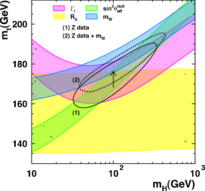
Figure 2: $m_{\mathrm{t}}$ and $m_{\mathrm{H}}$ constraints from Z-pole measurements and $m_{\mathrm{W}}$. Each band gives the $\pm 1\sigma$ constraint from the indicated measurement. The $\pm$ signs on each band show the sense of variation in the measurement. The arrow indicates the additional variation in $\sin^{2}\theta_{\mathrm{eff}}^{\mathrm{lept}}$ due to a $\pm 1\sigma$ uncertainty in $\Delta\alpha^{(5)}_{\mathrm{had}}(m_{\mathrm{Z}}^{2})$. The error contours are shown at 68% CL for fits to both the $\mathrm{Z}$-pole results alone (solid), and the $\mathrm{Z}$-pole results combined with $m_{\mathrm{W}}$ (dashed).

IV Higgsstrahlung

Since direct searches for the Higgs boson have demonstrated that $m_{\mathrm{H}}>114~{}\mathrm{GeV}$  at 95% CL LEP (2003), Figures 1 and 2 and Equation 13 follow the precision calculations of ZFITTER and TOPAZ0 in neglecting the Higgsstrahlung process shown in Figure 3.

Figure 3: Higgsstrahlung at the $\mathrm{Z}$-pole. The narrow width of the Higgs boson implies that its decay products have an invariant mass near $m_{\mathrm{H}}$, while the $\mathrm{Z}^{*}$ is sufficiently off-shell to ensure energy conservation.

However, the decrease of $\Delta\rho_{\mathrm{se}}$ at low $m_{\mathrm{H}}$ predicted by Equation 13 is due to the effect of virtual Higgs loops. These should properly be compensated by external Higgs corrections, which will enter with opposite sign. When choosing to ignore the direct Higgs search results to explore what the $\mathrm{Z}$-pole measurements alone tell us about the Standard Model, it is logically inconsistent to consider virtual Higgs corrections while neglecting the concomitant external corrections which the Standard Model predicts for low values of $m_{\mathrm{H}}$.

We have therefore undertaken calculations which account for the effects of the expected Higgsstrahlung at low $m_{\mathrm{H}}$. The fractional rate of such Higgsstrahlung is given in Franzini and Taxil (1989):

$$\frac{\Gamma(\mathrm{Z}\rightarrow H\,\mathrm{f\overline{f}})}{\Gamma(\mathrm{Z}\rightarrow\mathrm{f\overline{f}})}=\frac{\alpha}{4\,\pi\,\cos^{2}\theta_{\mathrm{W}}\,\sin^{2}\theta_{\mathrm{W}}}\times$$

$$\int_{2r}^{1+r^{2}}\frac{\left(1+\frac{2\,r^{2}}{3}-x+\frac{x^{2}}{12}\right)\,{\sqrt{x^{2}-4\,r^{2}}}}{\left(\frac{{\Gamma_{\mathrm{Z}}}^{2}}{{m_{\mathrm{Z}}}^{2}}+{\left(x-r^{2}\right)}^{2}\right)}dx\,,$$ (20)

where

$$x = 2E_{H}/m_{\mathrm{Z}}\,,$$ (21)

$$r = m_{\mathrm{H}}/m_{\mathrm{Z}}\,,$$ (22)

$$E_{H} = \frac{m_{\mathrm{Z}}^{2}+m_{\mathrm{H}}^{2}-m^{2}_{\mathrm{f\overline{f}}}}{2m_{\mathrm{Z}}}\,,$$ (23)

and $m_{\mathrm{f\overline{f}}}$ is the invariant mass of the $\mathrm{Z}^{*}$ decay products. The Higgsstrahlung of Equation 20 represents extra width for $\mathrm{Z}$ decay, which is not included in ZFITTER. Figure 4 shows the total width of the $\mathrm{Z}$ with and without this external Higgsstrahlung.

Figure 4: $\Gamma_{\mathrm{Z}}\,vs\,\log_{10}(m_{\mathrm{H}}/\mathrm{GeV})$, including and excluding external Higgsstrahlung.

At values of $m_{\mathrm{H}}$ below $\sim 50~{}\mathrm{GeV}$, which are still consistent with the $\mathrm{Z}$-pole measurements, the Standard Model Higgsstrahlung would have been appreciable, representing on the order of an $\mathrm{MeV}$ in the $\mathrm{Z}$ decay width.

In order to incorporate the effects of such Higgsstrahlung into the $\mathrm{Z}$-pole analysis, we re-interpret the experimental measurements, which we consider to include Higgsstahlung, in terms of the theoretical quantities as calculated by ZFITTER, without Higgsstrahlung. In the case of the total width this is particularly straight-forward:

$$\Gamma_{\mathrm{Z}}^{\mathrm{meas}}=\Gamma_{\mathrm{Z}}^{\mathrm{zf}}+\Gamma_{\mathrm{Z}}^{\mathrm{hs}}$$ (24)

where the superscripts have the obvious meanings: zf = ZFITTER, meas = measured, hs = Higgsstrahlung. Here $\Gamma_{\mathrm{Z}}^{\mathrm{hs}}=\Gamma(\mathrm{Z}\rightarrow H\,\mathrm{f\overline{f}})$, summed over all fermion species, is calculated according to Equation 20. Since $\Gamma_{\mathrm{Z}}$ is the resonance width of the $\mathrm{Z}$, determined by the decay lifetime and the uncertainty principle, its measurement is entirely independent of any details of the experimental event selection and analysis.

The manner in which the measurement of the partial widths will be affected is less obvious. Although experimental details differ among the four LEP collaborations, we take OPAL as a representative experiment Ahmet et al. (1991); Abbiendi et al. (2001) and study how Higgsstrahlung would have affected the measurements. Although it would be better to pursue these studies using detailed simulations of all four experiments, the precision which is necessary is sharply reduced by a very simple consideration: any Higgsstrahlung events classed as hadronic $\mathrm{Z}$ decays will simply increase the apparent value of $\alpha_{\mathrm{S}}$, and will otherwise not affect the analysis. This is the case since, while $\Gamma_{\mathrm{had}}$ and $\Gamma_{\ell\ell}$ share the same propagator corrections through $\Delta\rho_{\mathrm{se}}$, final-state QCD radiation increases the hadronic width alone by the factor $R_{\mathrm{QCD}}$:

$$R_{\mathrm{QCD}}=1+\frac{\alpha_{\mathrm{S}}}{\pi}+\cdots.$$ (25)

Any shift in the $\Gamma_{\mathrm{had}}/\Gamma_{\ell\ell}$ ratio is therefore interpreted by the fit as a change in $\alpha_{\mathrm{S}}$.

All four LEP experiments followed the natural strategy of essentially, if not formally, accepting all $\mathrm{Z}$ decays as hadronic unless they passed the stringent requirements to be identified as one of the three species of leptons. To an excellent approximation all Higgsstrahlung events in which the $\mathrm{Z}^{*}$ decays hadronically will remain classed as hadronic events. Since the dominant branching fraction of the Higgs boson in the relevant mass range is to $\mathrm{b\overline{b}}$, many other Higgsstrahlung events, except for very low values of $m_{\mathrm{H}}$, will also appear to be hadronic decays.

To clarify the experimental classification of the Higgsstrahlung events in which the $\mathrm{Z}^{*}$ decays leptonically we studied samples of fully simulated Higgstrahlung events in the OPAL detector. These samples were generated using the program HZHA-03 Janot (1989), included all accessible Higgs decays according to the Standard Model, and covered the $\mathrm{Z}^{*}$ decay channels $\mathrm{e}^{+}\mathrm{e}^{-}$, $\mu^{+}\mu^{-}$ and ${\mathrm{\nu\overline{\nu}}}$. Since $\mathrm{Z}^{*}$ decays to $\tau^{+}\tau^{-}$ were not available, we treated these as an average of $\mathrm{e}^{+}\mathrm{e}^{-}$ and $\mu^{+}\mu^{-}$.

For each $\mathrm{Z}^{*}$ decay channel, as a function of $m_{\mathrm{H}}$, we calculated the probability that the Higgstrahlung events would be classified as hadronic $\mathrm{Z}$ decays. If an event failed the hadronic selection, we assumed that it would be classified correctly according to the actual $\mathrm{Z}^{*}$ decay. Since the Standard Model assumes lepton universality, any cross-over between charged lepton channels would in any case be irrelevant.

We then calculated, as a function of $m_{\mathrm{H}}$, two fractions:

The fraction of Higgsstrahlung events, $\mathrm{F}^{had}_{\ell\ell}(m_{\mathrm{H}})$, in which the $\mathrm{Z}^{*}$ in fact decayed to charged leptons, but the event was identified as an hadronic $\mathrm{Z}$ decay.

The fraction of Higgsstrahlung events, $\mathrm{F}^{had}_{\mathrm{inv}}(m_{\mathrm{H}})$,in which the $\mathrm{Z}^{*}$ in fact decayed to neutrinos, but the event was identified as an hadronic $\mathrm{Z}$ decay.

Figure 5 displays these fractions along with a smooth function fitted to represent the Monte Carlo data.

Figure 5: As a function of $m_{\mathrm{H}}$, the fractions of Higgsstrahlung events where the $\mathrm{Z}^{*}$ in fact decayed, respectively, to charged leptons or neutrinos, but the event was identified as an hadronic $\mathrm{Z}$ decay.

We then calculate the measured partial widths, including the effects of Higgsstrahlung, using the smooth $\mathrm{F}^{had}_{\mathrm{xx}}$ functions:

$$\Gamma_{\mathrm{had}}^{\mathrm{meas}} = \Gamma_{\mathrm{had}}^{\mathrm{zf}}+\mathrm{F}^{had}_{\ell\ell}(m_{\mathrm{H}})\Gamma_{\ell\ell}^{\mathrm{hs}}+\mathrm{F}^{had}_{\mathrm{inv}}(m_{\mathrm{H}})\Gamma_{\mathrm{inv}}^{\mathrm{hs}}\,,$$ (26)

$$\Gamma_{\ell\ell}^{\mathrm{meas}} = \Gamma_{\ell\ell}^{\mathrm{zf}}+\left[1-\mathrm{F}^{had}_{\ell\ell}(m_{\mathrm{H}})\right]\Gamma_{\ell\ell}^{\mathrm{hs}}\,,$$ (27)

$$\Gamma_{\mathrm{inv}}^{\mathrm{meas}} = \Gamma_{\mathrm{inv}}^{\mathrm{zf}}+\left[1-\mathrm{F}^{had}_{\mathrm{inv}}(m_{\mathrm{H}})\right]\Gamma_{\mathrm{inv}}^{\mathrm{hs}}\,.$$ (28)

We take the effect of Higgsstrahlung on the measurement of $\sin^{2}\theta_{\mathrm{eff}}^{\mathrm{lept}}$ to be negligible. Clearly there is no effect on the SLD measurement of $A_{\mathrm{LR}}$, since it concerns only the initial state. Similarly, there can be no effect on the average $\tau$ polarization. The asymmetry measurements have a relative precision of at best a few percent, and any possible dilution of the asymmetry due to kinematic distortions in the few $10^{-3}$ fraction of Higgstrahlung events will not be significant.

With the relations of Equations 24 and 26-28, we then re-made the plot of Figure 1, using ZFITTER to calculate the measurement error bands and 68% CL contours for the re-intepreted measurements. The result is shown in Figure 6. Notice that the only visible change is the expected decrease in the slope of the $\Gamma_{\ell\ell}$ measurement band at low $m_{\mathrm{H}}$, due to failure of some leptonic Higgsstrahlung events to be identified as hadrons. The lower extremity of the 68% CL contour for the fit which drops the $A^{0,\,{\mathrm{b}}}_{\mathrm{FB}}$ measurement extends very slightly, reflecting the local shift in the $\Gamma_{\ell\ell}$ constraint. The lower $1\sigma$ error on $m_{\mathrm{t}}$ is only 2.4% larger than it was when Higgsstrahlung was ignored. As a test of our proceedures, we also carried out the same calculations assuming that all Higgsstrahlung was accepted as hadronic $\mathrm{Z}$ decay. As expected, the resulting plot was indistinguishable from Figure 1.

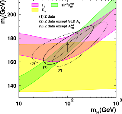
Figure 6: $m_{\mathrm{t}}$ and $m_{\mathrm{H}}$ constraints from Z-pole measurements with Higgsstrahlung taken into account. Each band gives the $\pm 1\sigma$ constraint from the indicated measurement. The arrow indicates the additional variation in $\sin^{2}\theta_{\mathrm{eff}}^{\mathrm{lept}}$ due to a $\pm 1\sigma$ uncertainty in $\Delta\alpha^{(5)}_{\mathrm{had}}(m_{\mathrm{Z}}^{2})$. The ellipses give the 68% CL fit contours for the indicated data.

In order to quantify the effect on $\alpha_{\mathrm{S}}$ of Higgsstrahlung being identified as hadronic $\mathrm{Z}$ decay, we performed a series of four-parameter fits, with $\alpha_{\mathrm{S}}$, $\alpha(m_{\mathrm{Z}}^{2})$, $m_{\mathrm{Z}}$, and $m_{\mathrm{t}}$ free, for a series of fixed $m_{\mathrm{H}}$ values. We plot the $1\sigma$ error bands of $\alpha_{\mathrm{S}}$ as a function of $\log_{10}(m_{\mathrm{H}}/\mathrm{GeV})$ in Figure 7, showing how $\alpha_{\mathrm{S}}$ shifts to compensate for the Higgsstrahlung which is identified as hadronic $\mathrm{Z}$ decay. Since $\Gamma_{\mathrm{had}}^{\mathrm{zf}}$, the hadronic width as re-interpreted for ZFITTER, is reduced from the fixed measured value, $\Gamma_{\mathrm{had}}^{\mathrm{meas}}$, by the Higgsstrahlung contribution, the hadronic final-state correction appears smaller, and the fit value of $\alpha_{\mathrm{S}}$ is reduced as $m_{\mathrm{H}}$ becomes small.

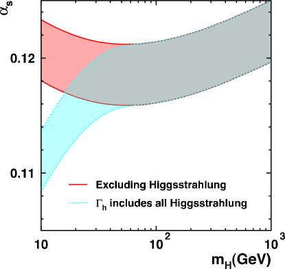
Figure 7: The $\pm 1\sigma$ error bands for $\alpha_{\mathrm{S}}$ found in the four-parameter fits as a function of $\log_{10}(m_{\mathrm{H}}/\mathrm{GeV})$, with and without Higgsstrahlung.

The $R_{\mathrm{b}}^{0}$ measurement band remains unchanged in Figure 6, since we have assumed that the Higgstrahlung events identified as hadrons do not disturb the quark flavor balance. Actually, since the Higgs boson decays predominantly to $\mathrm{b\overline{b}}$, it is likely that Higgsstrahlung will increase $\Gamma_{\mathrm{b\overline{b}}}$ proportionally more than the width of other flavors. A complete heavy flavor analysis was beyond the scope of this study, so we considered the limiting case that all Higgsstrahlung events where the Higgs boson decays to $\mathrm{b\overline{b}}$, and which are identified as hadrons, contribute to $\Gamma_{\mathrm{b\overline{b}}}$:

$$\Gamma_{\mathrm{b\overline{b}}}^{\mathrm{meas}}= \Gamma_{\mathrm{b\overline{b}}}^{\mathrm{zf}}+\mathrm{BR(Higgs}\rightarrow\mathrm{b\overline{b}})\times$$ (29)

$$\left[\mathrm{F}^{had}_{\ell\ell}(m_{\mathrm{H}})\Gamma_{\ell\ell}^{\mathrm{hs}}+\mathrm{F}^{had}_{\mathrm{inv}}(m_{\mathrm{H}})\Gamma_{\mathrm{inv}}^{\mathrm{hs}}\right]\,.$$

The result is shown in Figure 8.

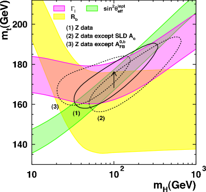
Figure 8: $m_{\mathrm{t}}$ and $m_{\mathrm{H}}$ constraints from Z-pole measurements with Higgsstrahlung taken into account. Here the assumption is made that all Higgstrahlung identified as hadrons contributes to $\Gamma_{\mathrm{b\overline{b}}}$. Each band gives the $\pm 1\sigma$ constraint from the indicated measurement. The arrow indicates the additional variation in $\sin^{2}\theta_{\mathrm{eff}}^{\mathrm{lept}}$ due to a $\pm 1\sigma$ uncertainty in $\Delta\alpha^{(5)}_{\mathrm{had}}(m_{\mathrm{Z}}^{2})$. The ellipses give the 68% CL fit contours for the indicated data.

The resulting dramatic upturn in the $\Gamma_{\mathrm{b\overline{b}}}$ measurement band flattens the lower extremity of the 68% CL contour for the $\mathrm{Z}$-pole fit in which the $A^{0,\,{\mathrm{b}}}_{\mathrm{FB}}$ measurement is dropped, but only modestly. The lower $1\sigma$ error on $m_{\mathrm{t}}$ for this fit is 11% smaller than it was when Higgsstrahlung was ignored. The corresponding shift in the lower $1\sigma$ error on $m_{\mathrm{t}}$ for the base fit including all $\mathrm{Z}$-pole measurements is only 1.7%. Other aspects of the error contours remain numerically unaffected.

V Conclusions

Our study of the manner in which the $\mathrm{Z}$-pole measurements constrain the Standard Model parameters $m_{\mathrm{t}}$ and $m_{\mathrm{H}}$ through their effect on radiative corrections shows that the measured leptonic width, $\Gamma_{\ell\ell}$ plays an important, and non-linear role. This non-linearity at low values of $m_{\mathrm{H}}$ contributes to a surprising stability in the agreement between the direct and indirect measurements of $m_{\mathrm{t}}$ under variations in $\sin^{2}\theta_{\mathrm{eff}}^{\mathrm{lept}}$. This singular demonstration of the consistency of our experimental and theoretical understanding of electroweak radiative corrections therefore remains undisturbed by the apparent discrepancy between the values of $\sin^{2}\theta_{\mathrm{eff}}^{\mathrm{lept}}$ derived from the measurements of $A^{0,\,{\mathrm{b}}}_{\mathrm{FB}}$ and $A_{\mathrm{LR}}$.

The neglect of external Higgstrahlung in ZFITTER and TOPAZ0 in the analysis of the $\mathrm{Z}$-pole measurements is found to have negligible impact on the central values of all the extracted Standard Model parameters, with the exception of $\alpha_{\mathrm{S}}$. Within a CL of 68% the error contours of these parameters also remain essentially unaffected.

References

- Ross and Veltman (1975) D. A. Ross and M. J. G. Veltman, Nucl. Phys. B95, 135 (1975).
- LEP (2003) Phys. Lett. B565, 61 (2003), eprint hep-ex/0306033.
- Bardin et al. (1989) D. Y. Bardin, M. S. Bilenkii, G. Mitselmakher, T. Riemann, and M. Sachwitz, Z. Phys. C44, 493 (1989).
- Bardin et al. (1990) D. Y. Bardin, M. S. Bilenkii, T. Riemann, M. Sachwitz, and H. Vogt, Comput. Phys. Commun. 59, 303 (1990).
- Bardin et al. (1991a) D. Y. Bardin et al., Nucl. Phys. B351, 1 (1991a), eprint arXiv:hep-ph/9801208.
- Bardin et al. (1991b) D. Y. Bardin et al., Phys. Lett. B255, 290 (1991b), eprint arXiv:hep-ph/9801209.
- Bardin et al. (1992) D. Y. Bardin et al., Zfitter: An analytical program for fermion pair production in annihilation (1992), eprint arXiv:hep-ph/9412201.
- Bardin et al. (2001) D. Y. Bardin et al., Comput. Phys. Commun. 133, 229 (2001), recently updated with results from Arbuzov (1999), eprint arXiv:hep-ph/9908433.
- Montagna et al. (1993a) G. Montagna, F. Piccinini, O. Nicrosini, G. Passarino, and R. Pittau, Nucl. Phys. B401, 3 (1993a).
- Montagna et al. (1993b) G. Montagna, F. Piccinini, O. Nicrosini, G. Passarino, and R. Pittau, Comput. Phys. Commun. 76, 328 (1993b).
- Montagna et al. (1996) G. Montagna, O. Nicrosini, G. Passarino, and F. Piccinini, Comput. Phys. Commun. 93, 120 (1996), eprint arXiv:hep-ph/9506329.
- Montagna et al. (1999) G. Montagna, O. Nicrosini, F. Piccinini, and G. Passarino, Comput. Phys. Commun. 117, 278 (1999), recently updated to include initial state pair radiation (G. Passarino, priv. comm.), eprint arXiv:hep-ph/9804211.
- Burkhardt and Pietrzyk (2001) H. Burkhardt and B. Pietrzyk, Phys. Lett. B513, 46 (2001).
- Veltman (1977) M. J. G. Veltman, Nucl. Phys. B123, 89 (1977).
- Abbiendi et al. (2001) G. Abbiendi et al. (OPAL), Eur. Phys. J. C19, 587 (2001), eprint arXiv:hep-ex/0012018.
- Burgers and Jegerlehner (1989) G. Burgers and F. Jegerlehner, in Z PHYSICS AT LEP 1. PROCEEDINGS, WORKSHOP, GENEVA, SWITZERLAND, SEPTEMBER 4-5, 1989. VOL. 1: STANDARD PHYSICS, edited by G. Altarelli, R. Kleiss, and C. Verzegnassi (CERN, Geneva, Switzerland, 1989), p. 55, yellow Report CERN 89-08.
- Jegerlehner (1991a) F. Jegerlehner, Prog. Part. Nucl. Phys. 27, 1 (1991a).
- Jegerlehner (1991b) F. Jegerlehner, in Testing the Standard Model - TASI-90, proceedings: Theoretical Advanced Study Institute in Elementary Particle Physics, Boulder, Colo., Jun 3-27, 1990, edited by M. Cvetic and P. Langacker (World Scientific, Singapore, 1991b), p. 916, pSI-PR-91-08.
- Bardin et al. (1999) D. Y. Bardin, M. Grünewald, and G. Passarino, Precision calculation project report (1999), eprint arXiv:hep-ph/9902452.
- Chetyrkin et al. (1995) K. Chetyrkin et al., in Reports of the working group on precision calculations for the Z resonance, edited by D. Bardin, W. Hollik, and G. Passarino (CERN, Geneva, Switzerland, 1995), CERN 95-03, p. 175, yellow Report CERN 95-03.
- (21) The LEP Collaborations ALEPH, DELPHI, L3, OPAL and the LEP Electroweak Working Group, and the SLD Heavy Flavour and Electroweak Groups, A Combination of Preliminary Electroweak Measurements and Constraints on the Standard Model, hep-ex/0312023.
- Abe et al. (2001) K. Abe et al. (SLD), Phys. Rev. Lett. 86, 1162 (2001), eprint arXiv:hep-ex/0010015.
- Hagiwara et al. (2002) K. Hagiwara et al. (Particle Data Group), Phys. Rev. D66, 010001 (2002).
- (24) Combination of CDF snd DØ Results on W Boson Mass and Width, Tevatron Electroweak Working Group and the CDF and DØ Collaborations, CDF Note 5888, DØ Note 3963, FERMILAB-FN-0716, July 2002.
- Franzini and Taxil (1989) P. Franzini and P. Taxil, in Z PHYSICS AT LEP 1. PROCEEDINGS, WORKSHOP, GENEVA, SWITZERLAND, SEPTEMBER 4-5, 1989. VOL. 2: HIGGS SEARCH AND NEW PHYSICS, edited by G. Altarelli, R. Kleiss, and C. Verzegnassi (CERN, Geneva, Switzerland, 1989), p. 84, yellow Report CERN 89-08.
- Ahmet et al. (1991) K. Ahmet et al. (OPAL), Nucl. Instrum. Meth. A305, 275 (1991).
-
Janot (1989)
P. Janot, in
Physics at LEP, CERN 96-01, vol. 2, edited by
T. S. G. Altarelli
and F. Zwirner
(CERN, Geneva, Switzerland,
1989), p. 309, for a
description of the updates and for the code see:
http://alephwww.cern.ch/janot/Generators.html. - Arbuzov (1999) A. B. Arbuzov, Light pair corrections to electron positron annihilation at lep/slc (1999), eprint arXiv:hep-ph/9907500.