WHITE PAPER REPORT on
Using Nuclear Reactors to Search for a value of $\theta_{13}$
January 2004

1. Academia Sinica, Taiwan

2. University of Alabama

3. Argonne National Laboratory

4. Lawrence Berkeley National Lab (Nuclear Science)

5. Lawrence Berkeley National Lab (Physics)

6. University of Bologna and INFN-Bologna, Italy

7. Centro Brasileiro de Pesquisas F sicas

8. University of California, Berkeley

9. California Institute of Technology

10. Universidade Estadual de Campinas

11. Catholic University of Rio de Janero

12. University of Chicago

13. Columbia University

14. Fermi National Accelerator Laboratory

15. College de France

16. Illinois Institute of Technology

17. IHEP Beijing

18. Kansas State University

19. Kurchatov Institute

20. Louisiana State University

21. Max-Plank-Institut für Kernphysik (Heidelberg)

22. Max-Plank-Institut für Physik (Munich)

23. University of Michigan

24. University of Minnesota at Crookston

25. Niigata University

26. Northwestern University

27. University of Pittsburgh

28. Rikkyo University

29. Saclay

30. SISSA Trieste

31. State University of New York, Stony Brook

32. University of Tennessee

33. Technical University Munich

34. University of Texas at Austin

35. Tohoku University

36. Tokyo Institute of Technology

37. Tokyo Metropolitan University

38. INFN Trieste

39. Virginia Tech

40. University of Washington

 

This document is available at
http://www.hep.anl.gov/minos/reactor13/white.html
or by writing:
Maury Goodman
HEP 362
Argonne Illinois 60439

Executive Summary

Purpose of this White Paper
There has been superb progress in understanding the neutrino sector of elementary particle physics in the past few years. It is now widely recognized that the possibility exists for a rich program of measuring CP violation and matter effects in future accelerator $\nu$ experiments, which has led to intense efforts to consider new programs at neutrino superbeams, off-axis detectors, neutrino factories and beta beams. However, the possibility of measuring CP violation can be fulfilled only if the value of the neutrino mixing parameter $\theta_{13}$ is such that $\sin^{2}(2\theta_{13})$ greater than or equal to on the order of 0.01. The authors of this white paper are an International Working Group of physicists who believe that a timely new experiment at a nuclear reactor sensitive to the neutrino mixing parameter $\theta_{13}$ in this range has a great opportunity for an exciting discovery, a non-zero value to $\theta_{13}$. This would be a compelling next step of this program. We are studying possible new reactor experiments at a variety of sites around the world, and we have collaborated to prepare this document to advocate this idea and describe some of the issues that are involved.

Purpose of the Experiment
In the presently accepted paradigm to describe the neutrino sector, there are three mixing angles. One is measured by solar neutrinos and the KamLAND experiment, one by atmospheric neutrinos and the long-baseline accelerator projects. Both angles are large, unlike mixing angles among quarks. The third angle, $\theta_{13}$, has not yet been measured to be nonzero but has been constrained to be small in comparison by the CHOOZ reactor neutrino experiment.

The basic feature of a new reactor experiment is to search for energy dependent $\bar{\nu}_{e}$ disappearance using two (or more) detectors, to see $\bar{\nu}_{e}\rightarrow\bar{\nu}_{e}$ disappearance. The detectors need to be located underground in order to reduce backgrounds from cosmic rays and cosmic ray induced spallation products. The detectors need to be designed identically in order to reduce systematic errors to 1% or less. Control of the relative detector efficiency, fiducial volume, and good energy calibration are needed.

A measurement of or stringent limit on $\theta_{13}$ would be crucial as part of a long term program to measure CP parameters at accelerators, even though a reactor $\bar{\nu}_{e}\rightarrow\bar{\nu}_{e}$ disappearance experiment does not measure any CP violating parameter. A sufficient value of $\theta_{13}$ measured in a reactor experiment would strongly motivate the investment required for a new round of accelerator $\nu$ experiments. A reactor experiment’s unambiguous measurement of $\theta_{13}$ would also strongly support accelerator measurements by helping to resolve degeneracies and ambiguities. The combination of measurements from reactors and neutrino results from accelerators will allow early probes for CP violation without the necessity of long running at accelerators with anti-neutrino beams.

Anticipated Sensitivity
The best current limit on $\theta_{13}$ comes from the CHOOZ experiment and is a function of $\Delta m^{2}_{atm}$, which has been measured using atmospheric neutrinos by Super-Kamiokande and others. The latest reported value of $\Delta m^{2}_{atm}$ from Super-Kamiokande is $1.2~{}<~{}\Delta m^{2}_{atm}~{}<~{}3.0~{}\times~{}10^{-3}$eV² with a best fit reported at 2.0. The CHOOZ limits for $\Delta m^{2}_{atm}$ of 2.6 and 2.0 $\times~{}10^{-3}$eV² are $\sin^{2}(2\theta_{13})~{}<~{}$ 0.14 and 0.20. Global fits using the solar data limit the value for small $\Delta m^{2}_{atm}$ to less than 0.12. In order to improve on the CHOOZ experiment, a new reactor experiment needs more statistics and better control of systematic errors. The relative sensitivity at low $\Delta m^{2}_{atm}$ can be improved by locating the far detector further than 1 km. Increased statistics can be achieved by running longer, using a larger detector, and judicious choice of a nuclear reactor. The dominant systematic errors in an absolute measurement of the reactor neutrino flux, such as cross-sections, flux uncertainties, and the absolute target volume, will be largely eliminated in a relative measurement with two or multiple detectors. Good understanding of the relative detector response and the backgrounds is required for a precise relative measurement of the reactor neutrino flux and spectrum. Experiments are being considered which increase the luminosity from the CHOOZ value of 12 t GW y (ton-Gigawatt-years) to 400 t GW y or more. This will allow a mixing angle sensitivity of $\sin^{2}(2\theta_{13})~{}>~{}0.01$. For example, 400 t GW y would be obtained with a 10 (40) ton far detector, and a 14 (3.5) GW reactor in 3 years. One design consideration of the new experiment is the possibility for upgrades to achieve even greater luminosity and sensitivity. The ability to phase upgrades to achieve a luminosity of 8000 t GW y is being considered.

Major Challenges
A new reactor experiment will build on the experience of several previous reactor experiments, such as CHOOZ, Palo Verde and KamLAND (described in Section 4 of this white paper). These experiments had different goals, mostly being designed for signals due to large mixing. Important experience on calibration, control of systematic errors and the reduction of background has also been obtained by the Super-Kamiokande, SNO and Borexino collaborations.

A next-generation reactor experiment will be designed to make a precision measurement of the reactor electron anti-neutrino survival probability at different distances from the reactor and search for subdominant oscillation effects associated with the mass splitting of the m₁ and m₃ mass eigenstates. A measurement at the $\mathcal{O}$(1%) level will require careful control of possible systematic errors. Most of the technical requirements of this experiment are well understood but the details of the detector design still need to be optimized. Some of the open questions under consideration are the following: liquid scintillator loaded with 0.1% of gadolinium has been used in the past, but there are concerns regarding its stability in solution and possible attenuation length degradation which need to be fully understood. If movable detectors are chosen, there must be confidence that moving the detector does not introduce additional time-dependent effects. The use of a second detector will certainly help to control many systematic errors, but also will present a challenge in maintaining a known relative calibration over time. Another challenge is reduction of cosmic ray associated backgrounds such as neutrons and ⁹Li spallation and their accurate estimation. The reduction of gamma ray background is also important because it will affect the ability to reduce the threshold to below 1 MeV. These and other design issues are discussed in Sections 5-8 of this white paper.

Experimental Prospects
The International Working Group has held two workshops (April 30-May 1, 2003 at the University of Alabama and October 9-11, 2003 at Technical University of Munich) and we are planning a third one (March 20-22, 2004 at Niigata University.) During the past year, the International Working Group has identified a large number of reactors as possible sites for a new experiment. Many of these sites are discussed in Section 9, and a few are described in more detail in seven Appendices. These include the Angra reactor in Brazil; the possibility of a new experiment at CHOOZ, called Double-CHOOZ (or CH$\theta_{13}\theta_{13}$Z); Daya Bay near Hong Kong in China, Diablo Canyon in California; a reactor in Illinois; the reactor complex at Kashiwazaki in Japan, and the Krasnoyarsk reactor underground at Zhelezhnogorsk in Russia.

It is not the role of this document to provide a cost estimate or schedule for any of the experiments which will be proposed. But it is appropriate to try to set the scale of the endeavor in order to compare to other kinds of initiatives in neutrino physics. A two-detector system as described in this document seems to cost in the range $5M to $15M. The civil construction costs to place these detectors underground will be very site dependent and require a detailed engineering cost estimate as described in Section 11. Estimates are in the range of several tens of millions of dollars, depending on site condition and tunnel length. Since reactors with an underground site already exist, such as those at CHOOZ and Krasnoyarsk, there is a strong incentive to consider those sites for the earliest experiment, though there may be physics trade-offs which must be considered. Some of the envisioned reactor experiments might start taking data in 2007-2008. First results could be achieved as early as 2009.

None of these efforts has yet resulted in a proposal to a funding agency, but site specific proposals and R&D proposals will be submitted during 2004. This white paper is a step in that direction. Given the importance of the measurement of $\theta_{13}$ and the enthusiasm of the proponents, we are hopeful that two or more of these experiments will move forward on a favorable time scale.

1 Introduction

The discovery of neutrino oscillations is a direct indication of physics beyond the Standard Model and it provides a unique new window to explore physics at high mass scale including unification, flavor dynamics, and extra dimensions. The smallness of neutrino masses and the large lepton flavor violation associated with neutrino mixing are both fundamental properties that give insights into modifications of current theories. Other possibilities that may reveal themselves in the neutrino sector include extra “sterile” neutrinos, CP violation in the neutrino mixing matrix, and CPT violation associated with the neutrino mass hierarchy. Since neutrino oscillations have now been established, the next step is to map out the parameters associated with neutrino masses and mixings. The experimental program to accomplish this goal will require a wide range of experiments using neutrinos from solar, atmospheric, reactor, and accelerator sources. Due to the relations between these various measurements, it will be important for the world-wide community to set up a structured program to work through the experimental measurements in a coherent and logical manner.

The existing experimental results fit rather nicely into a picture with three massive neutrinos, which corresponds to the simplest scenario for three generations (for recent global analyses see, e.g., References [1, 2]). Neutrino oscillations then involve two mass-squared differences ($\Delta m^{2}_{21}$ and $\Delta m^{2}_{32}$, where $\Delta m^{2}_{ij}=m(\nu_{i})^{2}-m(\nu_{j})^{2}$), three mixing angles ($\theta_{12}$, $\theta_{23}$, and $\theta_{13}$), and a CP-violating phase ($\delta$). The present status of these parameters is summarized in Figure 1. Atmospheric neutrino data [3] and the first results from the K2K long-baseline accelerator experiment [4] determine $|\Delta m^{2}_{32}|=(2^{+1.2}_{-0.9})\times 10^{-3}$ eV² (errors at $3\sigma$) and $\theta_{23}\approx 45^{\circ}$ [3, 2], whereas most solar data [5, 6], combined with the results from the KamLAND reactor experiment [7], lead to $\Delta m_{21}^{2}=(6.9^{+2.6}_{-1.5})\times 10^{-5}$ eV² and $\sin^{2}\theta_{12}=0.3^{+0.09}_{-0.07}$ at $3\sigma$ [1].

The neutrino sector may contain more than three neutrinos by including mixing to sterile neutrinos (for example to account for the LSND [8] anomaly), but in these cases the mixing matrix most likely factors to a good approximation into a $(3\times 3)$ submatrix with the parameters given above. The investigation of oscillations involving sterile neutrinos will demand measurements such as MiniBooNE as well as improved disappearance measurements at high $\Delta m^{2}$.

The current experimental situation can thus be summarized by two more or less decoupled oscillations governed by the “atmospheric” and “solar/reactor” quadratic mass splittings $\Delta m^{2}_{atm}=\Delta m^{2}_{13}$ and $\Delta m^{2}_{sol}=\Delta m^{2}_{21}$, respectively, and the corresponding mixing angles $\theta_{12}=\theta_{sol}$ and $\theta_{23}=\theta_{atm}$, which turned out to be surprisingly large. This leads in the future to two equally important experimental directions: The first task is to improve the knowledge of the above (leading) oscillation parameters and to make precision measurements. Conceptually at least equally important is the fact that three flavors imply also three flavor oscillations and thus one further mixing angle, $\theta_{13}$ as well as a CP violating phase $\delta$ . The CP phase $\delta$ is a very interesting, but so far a completely unknown, parameter. The fact the LMA solution has been confirmed means that $\delta$ is in principle accessible in future experiments if $\theta_{13}$ is not too small. In many models of neutrino masses the see-saw mechanism leads to connections of the leptonic CP phase $\delta$ to the CP phases in the heavy Majorana sector and thus to leptogenesis, one of the best known mechanism to explain the baryon asymmetry of the universe (see e.g. [9]). Neutrino masses may therefore explain a second indication for physics beyond the Standard Model, since the observed baryon asymmetry cannot be generated from CP violation in the Standard Model with massless neutrinos. Future neutrino experiments aim therefore indirectly at another key question in physics, namely what causes the baryon asymmetry in the Universe.

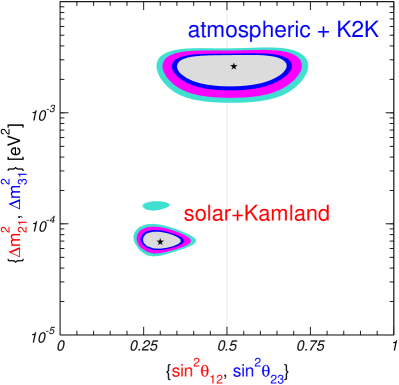
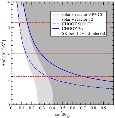
Figure 1: Status of neutrino oscillation parameters from a combined analysis of current global data [1]. Left panel: allowed regions of solar ($\Delta m^{2}_{21},\sin^{2}\theta_{12}$) and atmospheric ($\Delta m^{2}_{31},\sin^{2}\theta_{23}$) parameters at 90%, 95%, 99% and $3\sigma$ CL. Right panel: upper bound on $\sin^{2}2\theta_{13}$ from the CHOOZ experiment at 90% (dashed) and $3\sigma$ (solid) CL for 1 DOF as a function of $\Delta m^{2}_{31}$. The light (dark) shaded region is excluded from CHOOZ + solar + KamLAND data at 90% ($3\sigma$) CL for 1 DOF. The horizontal lines indicate the current best fit value and the $3\sigma$ allowed regions for $\Delta m^{2}_{31}$.

The mixing angle $\theta_{13}$, the parameter relevant for three flavor effects in neutrino oscillations, is known to be small from the CHOOZ [10, 11] and also from the Palo Verde experiment [12]. The current bound from global data is summarized in the right hand panel of Figure 1. It depends somewhat on the true value of the atmospheric mass squared difference, since the bound from the CHOOZ experiment gets rather weak for $\Delta m^{2}_{31}\lesssim 2\times 10^{-3}$ eV². However, in that region an additional constraint on $\theta_{13}$ from global solar neutrino data becomes important [1]. At the current best fit value of $\Delta m^{2}_{31}=2\times 10^{-3}$ eV² we have the bounds at 90% ($3\sigma$) CL for 1 DOF

$$\sin^{2}2\theta_{13}\leq 0.16~{}(0.25)\,,\quad\sin^{2}\theta_{13}\leq 0.053~{}(0.066)\,,\quad\theta_{13}\leq 10.8^{\circ}~{}(14.9^{\circ})\,.$$ (1)

Genuine three flavor oscillation effects occur only for a finite value of $\theta_{13}$ and establishing a finite value of $\theta_{13}$ is therefore one of the next milestones in neutrino physics. Leptonic CP violation is also a three flavor effect, but it can only be tested if $\theta_{13}$ is finite. There is thus a very strong motivation to establish a finite value of $\theta_{13}$ in order to aim in the long run at a measurement of leptonic CP violation (see e.g. [13, 14]).

Future measurements of $\bar{\nu}_{e}$ disappearance using a two detector reactor experiment and long-baseline $\nu_{\mu}\rightarrow\nu_{e}$ and $\bar{\nu}_{\mu}\rightarrow\bar{\nu}_{e}$ experiments will be crucial in determining $\theta_{13}$, the sign of $\Delta m_{32}^{2}$, and the CP phase $\delta$. If $\theta_{13}\gtrsim 0.01$, the design of experiments to measure the sign of $\Delta m_{32}^{2}$ and the CP phase $\delta$ become straight forward extensions of current experiments. For this reason, there is general agreement that a $\theta_{13}$ measurement should be the prime goal of the next round of experiments. On the theoretical side these experiments could test if the small value of $\theta_{13}$ could be a numerical coincidence or if e.g. some symmetry argument is required to explain a tiny value.

Future measurements of $\theta_{13}$ are possible using reactor neutrinos and accelerator neutrino beams. As will be shown in subsequent sections, reactor measurements have the property of determining $\theta_{13}$ without the ambiguities associated with matter effects and CP violation. In addition, the needed detector for an initial reactor measurement is small ($\lesssim 50$ tons) and the construction of a neutrino beam is not necessary. For this reason, a precision reactor experiment could lead the way in establishing the future oscillation program by setting the scale of the $\theta_{13}$ mixing angle. The previous most accurate measurements were by the CHOOZ and Palo Verde experiments where a single detector was placed about 1 km from the reactor. Future reactor experiments using two detectors ($\sim 50$ tons) at near (100 - 200 m) and far (1 - 2 km) locations will have significantly improved sensitivity for $\theta_{13}$ down to the 0.01 level. With $\theta_{13}$ determined, measurements of $\nu_{\mu}\rightarrow\nu_{e}$ and $\bar{\nu}_{\mu}\rightarrow\bar{\nu}_{e}$ oscillations using accelerator neutrino beams impinging on large detectors at long baselines will improve the knowledge of $\theta_{13}$ and also allow access to matter or CP violation effects. For the field to exploit the physics opportunities available for neutrino oscillation measurements, it is clear that a suite of experiments including both reactor and long-baseline accelerator measurements will be necessary.

In addition to the general physics arguments, there are two factors that lend urgency to this initiative. Our studies indicate that a reactor experiment to measure $\sin^{2}2\theta_{13}$ to the level of 0.01 could be done at significantly less cost and on a more rapid time scale than an accelerator long-baseline neutrino experiment with comparable sensitivity. This conclusion is influenced by several recent developments, including the High Energy Physics Roadmap for the future, February 2002 [16], the prioritizations made in “High Energy Physics Facilities on the DOE Office of Science Twenty-Year Roadmap” issued by the U.S. Department of Energy in March, 2003 [17] and the “Facilities for the Future of Science: a Twenty-year Outlook” issued by the Office of Science of the DOE in November, 2003 [18]. In particular, the latter document envisions that a high-intensity neutrino beam is more than 15 years in the future. For comparison with an off-axis long baseline experiment, we use cost and time estimates based on current work for the Fermilab proposal P929, the NuMI Off-Axis Experiment. We emphasize that a new reactor experiment does not reduce the motivation for the latter experiment; it obtains information complementary to that obtained by the reactor $\theta_{13}$ experiment, such as the mass hierarchy between $m(\nu_{3})$ and $m(\nu_{1})$. Instead, we would envision that, since the reactor experiment can be performed more quickly, its findings concerning $\theta_{13}$ will provide very important guidance for the long baseline program.

In this White Paper, we outline the capabilities of next generation reactor experiments and summarize the design considerations that groups are considering in developing this program. The International Working Group on $\theta_{13}$ is sharing ideas on how to best design a new reactor experiment, and one goal of this White Paper is to document the present status of our understanding of these issues.

In the next section, we discuss in more detail the physics opportunities and the motivation for a new reactor experiment. The following Section 3 deals with the optimal baseline, luminosity scaling and the impact of systematic errors. Previous reactor experiments are described in Section 4, and in Section 5 we present some thoughts about the general layout of the detector, a multi-layered volume of scintillator designed to define the fiducial volume well, and also carefully control other potential systematic errors. In Section 6, the calibration requirements for the detector are reviewed. Section 7 considers the issues of backgrounds and how they affect the required overburden. Depths that provide an overburden of 400 mwe to 1100 mwe are desirable. The goal of carefully minimizing systematic errors is qualitatively different than has been required of neutrino experiments at reactors in the past. We are confident that the two detector concept will provide lower systematic errors than have been previously achieved, but the ultimate limit on achievable systematic error has yet to be identified. A discussion of a variety of systematic errors is presented in Section 8. Characteristics of a large number of sites are reviewed in Section 9 and some more detailed experimental site plans for seven of the possible locations are included in the Appendices to this document. Next we discuss other physics that can be done in Section 10. Depending on the site, the costs of a new reactor experiment will potentially be dominated by the civil construction of a shaft or tunnel. Those civil engineering issues are reviewed in Section 11. Safety issues are discussed in Section 12. Section 13 is finally devoted to outreach and educational issues. The appendices contain further details of potential sites.

2 Physics Opportunities and Motivation

2.1 Road Map for Future Neutrino Oscillation Measurements

There is now a world-wide experimental program underway to measure the parameters associated with neutrino oscillations. The current experiments include K2K that measures $\nu_{\mu}$ disappearance over a 250 km baseline from KEK to SK. Another experiment is MiniBooNE that is searching for $\nu_{\mu}\rightarrow\nu_{e}$ appearance signal in the LSND $\Delta m^{2}$ region from 0.2 to 1 eV². Upcoming longer-baseline ($\sim 700$ km) experiments are NuMI/MINOS at Fermilab and CNGS at CERN that will study $\nu_{\mu}$ oscillations in the atmospheric $\Delta m^{2}$ region. Groups in all the world-wide regions are also pursuing sites and experiments for a precision reactor experiment using detectors with fiducial volumes of 5 to 50 ton. Several near-term new long-baseline experiments are planned which will use off-axis beams including the approved J-PARC (previously called JHF) to Super-K (22.5 kton) experiment and the developing NuMI off-axis experiment (50 kton detector). Following these experiments, the next stage might be neutrino superbeam experiments with even longer baselines that could possibly be combined with large proton decay detectors. Four such projects under consideration are: (i) BNL with an AGS upgrade, (ii) Fermilab with a proton driver upgrade, (iii) J-PARC (phase II), and (iv) a CERN Superconducting Proton LINAC experiment. Future neutrino factories, using a muon storage ring, will provide the ultimate in sensitivity and precision in oscillation measurements.

It is clear that developments in the field will dictate how the community should proceed through these studies. As stated previously, the size of $\theta_{13}$ is the small parameter that sets the scale for further studies in a three neutrino scenario. It is also clear that the final resolution of the LSND anomaly by MiniBooNE could significantly affect the direction for new investigations. To bring this information together in a coherent way, we present a roadmap for neutrino oscillations which tries to point out the relations between the various measurements:

• Stage 0: The Current Program

  • There are improved measurements of $\Delta m_{12}^{2}$ (5-10%) by solar neutrino and the KamLAND experiments.

  • NuMI, CNGS, and K2K experiments check the atmospheric oscillation phenomenology and measure $\Delta m_{23}^{2}$to $\sim 10$%.

  • MiniBooNE makes a definitive check of the LSND effect and measures the associated $\Delta m^{2}$ if the effect is confirmed.

• Stage 1: Measurement or tight constraint’s on the $\theta_{13}$ angle
  

  • The NuMI/MINOS on-axis experiment probes $\sin^{2}2\theta_{13}>0.06$ at 90% CL.

  • Two-detector, long-baseline reactor experiments probe $\sin^{2}2\theta_{13}>0.01$ at 90% CL.

  • The NuMI and J-PARC off-axis experiments with 20-50 kton detectors investigate $\nu_{\mu}\rightarrow\nu_{e}$ transitions for oscillation probabilities greater than 1%.

• Stage 2: Measurements of the sign of $\Delta m_{23}^{2}$ and CP violation using superbeams and very large detectors (500 to 1000 kton)
  (This is feasible if $\sin^{2}2\theta_{13}>0.01$ and if $\delta$ is large enough.)

  • Measurements of $\nu_{\mu}\rightarrow\nu_{e}$ at several baselines need to be combined with either precision reactor measurements of $\nu_{e}\rightarrow\nu_{e}$ or with $\bar{\nu}_{\mu}\rightarrow\bar{\nu}_{e}$

  • Increased neutrino beam rates are needed, especially for the $\bar{\nu}_{\mu}$ running, which make high intensity proton sources necessary.

• Stage 3: Measurements with a Neutrino Factory

  • New facilities probe a mix of $\overset{(-)}{\nu}_{\mu/e}\rightarrow\overset{(-)}{\nu}_{e/\mu}$ transitions with sensitivities below the 0.001 level

  • They also map out CP violation with precision for $\sin^{2}2\theta_{13}>0.001$.

A flow chart with these ideas is shown in Figure 2.

Figure 2: Flow chart for a possible future neutrino program

2.2 Where do reactor oscillation experiments fit in?

Any oscillation effect in $\bar{\nu}_{e}$ survival is governed, assuming three flavor mixing, by the equation

$$P(\bar{\nu}_{e}\rightarrow\bar{\nu}_{e})\cong 1-\sin^{2}2\theta_{13}\sin^{2}(\frac{\Delta m^{2}_{atm}L}{4E})-\cos^{4}\theta_{13}\sin^{2}2\theta_{12}\sin^{2}(\frac{\Delta m^{2}_{12}L}{4E}).$$ (2)

This equation is plotted in Figure 3 as a function of $\mathrm{L/E}$ with the current best values for the $\Delta m^{2}$s and mixing angles ($\sin^{2}(2\theta_{13})$ is set to the maximum value allowed by current limits).

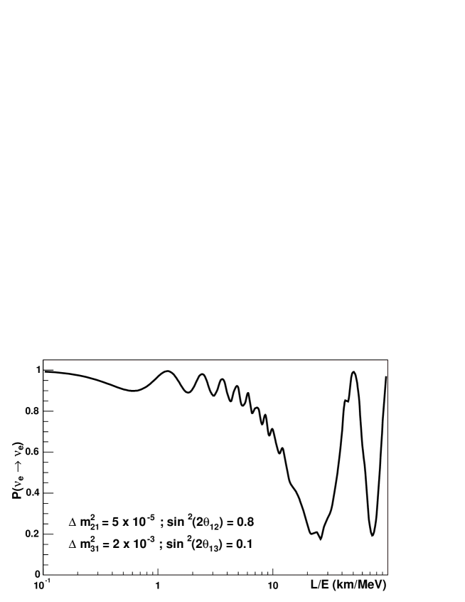
Figure 3: Probability of $\nu_{e}$ disappearance versus $\mathrm{L/E}$ for $\theta_{13}$ at its current upper limit

One can clearly see the two oscillations governed by the two $\Delta m^{2}$s. Experimentally, a judicious choice of $\mathrm{L/E}$ should be able to distinguish one effect from the other. The KamLAND experiment is the first reactor experiment to see oscillation effects, by measuring a 40% disappearance of $\bar{\nu}_{e}$. Given that the average baseline for KamLAND is 180 km, the detected deficit is presumably associated with the third ($\Delta m^{2}_{12}$) term in Equation (2).

The current best limit on $\theta_{13}$ comes from a lack of observed oscillations at CHOOZ and Palo Verde ($\sin^{2}2\theta_{13}<0.20$ for $\Delta m^{2}_{atm}~{}=~{}2.0\times 10^{-3}$eV²). These experiments were at a baseline distance of about 1 km and thus more sensitive to the second ($\Delta m^{2}_{atm}$) term of Equation (2). Those experiments could not have had greatly improved sensitivity to $\theta_{13}$ because of uncertainties related to knowledge of the flux of neutrinos from the reactors. They were designed to test whether the atmospheric neutrino anomaly might have been due to $\nu_{\mu}\rightarrow\nu_{e}$ oscillations, and hence were searching for large oscillation effects.

Since the effective disappearance will be very small (see Figure 3), any new experiment which is designed to look for non-zero values of $\theta_{13}$ would need to move beyond the previous systematic limitations. This could be achieved by utilizing the following properties:

• two or more detectors to reduce uncertainties to the reactor flux

• identical detectors to reduce systematic errors related to detector acceptance

• carefully controlled energy calibration

• low backgrounds and/or reactor-off data

Note that CP violation does not affect a disappearance experiment, and that the short baseline distances involved in a reactor measurement of oscillations at the atmospheric $\Delta m^{2}$ allow us to safely ignore matter effects.

A next generation reactor oscillation experiment would use at least two detectors placed at various distances from a high power reactor (Figure 4). The reactor provides a high intensity, isotropic source of neutrinos with a well-known spectrum as shown in Figure 5. The neutrino cross section for this process is well known as described in Reference [19]. Antineutrinos are detected through the inverse-$\beta$ decay process followed by neutron capture.

$$\bar{\nu}_{e}+p\rightarrow e^{+}+n.$$

The detector would most likely be composed of a vat of scintillator oil viewed from its surface by an array of photomultipliers. In order to reduce the background from cosmic-ray spallation, the detectors will need to be underground with at least 300 mwe of shielding. A detected event would correspond to a coincidence signal of an electron and capture neutron. The incident neutrino energy is directly related to the measured energy of the outgoing electron. The search for oscillations would then involve comparing the neutrino rate in the two detectors and looking for a non-$1/r^{2}$ dependence.

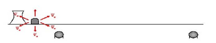
Figure 4: Schematic layout of a two detector reactor neutrino oscillation experiment.

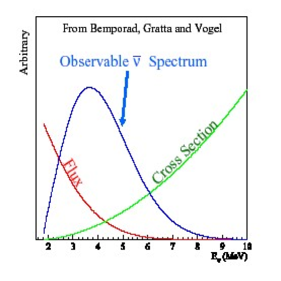
Figure 5: Antineutrino flux, cross section, and relative event rate using a reactor source [20].

As stated above, $\theta_{13}$ is a key parameter in developing the future neutrino oscillation program. Reactor experiments offer a straightforward and cost effective method to measure or constrain the value of this parameter. The sensitivity of a two detector experiment is comparable to that of the proposed initial off-axis long-baseline experiment. Since a reactor experiment would be much smaller and use an existing reactor neutrino source with a well understood neutrino rate, the experiment should be able to be done fairly quickly and at reduced costs. It is likely that an early measurement of $\theta_{13}$ will be necessary before the community invests a large amount of resources for a full off-axis measurement. For the longer term, a reactor experiment would be complementary to the off-axis experiments in separating the measurement of $\theta_{13}$ from other physics parameters associated with matter effects and CP violation. A follow-up reactor experiment with much larger detectors at various baselines will continue to be an important component of the neutrino oscillation program.

2.3 Reactor experiment as a clean laboratory for the $\theta_{13}$-measurement

In this section, we demonstrate that a reactor measurement of $\theta_{13}$ is a clean measurement which is free from any contamination, such as from effects of the other mixing parameters or from the Earth matter effect [84]. This key feature is one of the most important advantages of the reactor experiments. We use the standard notation of the lepton flavor mixing matrix:

$$U=\left[\begin{array}[]{ccc}c_{12}c_{13}&s_{12}c_{13}&s_{13}e^{-i\delta}\\ -s_{12}c_{23}-c_{12}s_{23}s_{13}e^{i\delta}&c_{12}c_{23}-s_{12}s_{23}s_{13}e^{i\delta}&s_{23}c_{13}\\ s_{12}s_{23}-c_{12}c_{23}s_{13}e^{i\delta}&-c_{12}s_{23}-s_{12}c_{23}s_{13}e^{i\delta}&c_{23}c_{13}\\ \end{array}\right].$$ (6)

Due to the low neutrino energy of a few MeV, the reactor experiments are inherently disappearance experiments, i.e., they can only measure the survival probability $P(\bar{\nu}_{e}\rightarrow\bar{\nu}_{e})$. Unlike the case of the $\nu_{e}$ appearance probability, it is well-known that the survival probability does not depend on the CP phase $\delta$ in arbitrary matter densities (for more details, see [84]). For reactor experiments, the matter effect is very small because the energy is quite low and the effect can be ignored to a good approximation. This can be seen by the comparison of the matter and the vacuum effects

$$\frac{a}{|\frac{\Delta m^{2}_{31}}{2E}|}=3.4\cdot 10^{-4}\left(\frac{|\Delta m^{2}_{31}|}{2.5\cdot 10^{-3}\,\mbox{eV}^{2}}\right)^{-1}\left(\frac{E}{4\,\mbox{MeV}}\right)\left(\frac{\rho}{2.8\,\mbox{g}\cdot\mbox{cm}^{-3}}\right)\left(\frac{Y_{e}}{0.5}\right).$$ (7)

Here $E$ is the neutrino energy. In addition, $a=\sqrt{2}G_{F}N_{e}$ denotes the index of refraction in matter with the Fermi constant $G_{F}$ and the electron number density $N_{e}$ in the Earth (which is related to the Earth matter density $\rho$ by $N_{e}=Y_{e}\rho/m_{p}$ with the proton fraction $Y_{e}$).

Since we know that the matter effect is negligible, we immediately understand that the survival probability is independent of the sign of $\Delta m^{2}_{31}$. Therefore, one can use the vacuum probability formula for the analysis of a reactor measurement of $\theta_{13}$. The expression for $P(\bar{\nu}_{e}\rightarrow\bar{\nu}_{e})$ in vacuum is given by [21]

$$1-P(\bar{\nu}_{e}\rightarrow\bar{\nu}_{e}) = \sin^{2}{2\theta_{13}}\sin^{2}\Delta_{31}$$ (8)

$$+ 1/2\,c^{2}_{12}\sin^{2}{2\theta_{13}}\sin{2\Delta_{31}}\sin{2\Delta_{21}}$$

$$+ c^{4}_{13}\sin^{2}{2\theta_{12}}\sin^{2}{\Delta_{21}}$$

$$+ c^{2}_{12}\sin^{2}{2\theta_{13}}\cos{2\Delta_{31}}\sin^{2}{\Delta_{21}},$$

where $\Delta_{ij}\equiv\Delta m_{ij}^{2}L/(4E)$ and $c_{ij}=\cos\theta_{ij}$. Defining the mass hierarchy parameter $\alpha$ as $\alpha\equiv\Delta m^{2}_{21}/\Delta m^{2}_{31}$, where $|\alpha|\simeq 0.03$, the second term in Equation (8) is suppressed relative to the main depletion term (first term) by a factor of $|\alpha|\,\sin^{2}{2\theta_{13}}\leq 6\times 10^{-3}$, the fourth term even by a factor of $\alpha^{2}\,\sin^{2}{2\theta_{13}}$. Thus, we can re-write Equation (8) for $\Delta_{21}\ll 1$ (for the baselines considered) as

$$1-P(\bar{\nu}_{e}\rightarrow\bar{\nu}_{e})\quad\simeq\quad\sin^{2}2\theta_{13}\,\sin^{2}\Delta_{31}+\alpha^{2}\,\Delta_{31}^{2}\,c^{4}_{13}\,\sin^{2}2\theta_{12}.$$ (9)

Though the second term on the right-hand side of this equation could be of the order of the first term for very large $|\alpha|$, it can be neglected for the first atmospheric oscillation maximum (where the first term is large) and $\sin^{2}2\theta_{13}$ larger than about $10^{-3}$. Therefore, the disappearance probability can be well approximated by the two-flavor depletion term in vacuum, which is the first term in Equation (8). Assuming that $|\Delta m^{2}_{31}|$ is accurately determined by a long-baseline $\nu_{\mu}$ disappearance measurement, the reactor experiments thus serve for a clean measurement of $\theta_{13}$ independent of other mixing parameters.

2.4 Comparison to superbeams

We have demonstrated in the last section that reactor measurements allow a degeneracy-free measurement of $\sin^{2}2\theta_{13}$. In order to qualitatively discuss the difference between reactor experiments and superbeams, we can compare the oscillation probabilities of the dominant oscillation channels. For the superbeams, one can expand the appearance probability $P_{\mu e}$ (or $P_{\bar{\mu}\bar{e}}$) in terms of the small mass hierarchy parameter $\alpha\equiv\Delta m_{21}^{2}/\Delta m_{31}^{2}$ and the small mixing angle $\sin 2\theta_{13}$ using the standard parameterization of the leptonic mixing matrix $U$ in Equation (6). As a first approximation for a qualitative discussion, one can use the vacuum formula from References [14, 22, 23] with the terms up to the second order (i.e., proportional to $\sin^{2}2\theta_{13}$, $\sin 2\theta_{13}\cdot\alpha$, and $\alpha^{2}$):

$$P_{\mu e} \simeq |\sin 2\theta_{13}\,\sin\theta_{23}\sin{\Delta_{31}}e^{i(\Delta_{32}\pm\delta_{\mathrm{CP}})}+\cos\theta_{13}\,\cos\theta_{23}\sin 2\theta_{12}\sin{\Delta_{21}}|^{2}$$ (10)

$$\approx \sin^{2}2\theta_{13}\,\sin^{2}\theta_{23}\sin^{2}{\Delta_{31}}$$

$$\mp\alpha\;\sin 2\theta_{13}\,\sin\delta_{\mathrm{CP}}\,\cos\theta_{13}\sin 2\theta_{12}\sin 2\theta_{23}\,\Delta_{31}\sin^{2}{\Delta_{31}}$$

$$+\alpha\;\sin 2\theta_{13}\,\cos\delta_{\mathrm{CP}}\,\cos\theta_{13}\sin 2\theta_{12}\sin 2\theta_{23}\,\Delta_{31}\cos{\Delta_{31}}\sin{\Delta_{31}}$$

$$+\alpha^{2}\,\cos^{2}\theta_{23}\sin^{2}2\theta_{12}\,\Delta^{2}_{31}.$$

Here $\Delta_{ij}\equiv\Delta m_{ij}^{2}L/(4E)\equiv(m_{i}^{2}-m_{j}^{2})L/(4E)$ and the sign of the second term refers to neutrinos (minus) or antineutrinos (plus). We have used the approximations that $\sin\Delta_{21}\simeq\alpha\Delta_{31}\ll 1$ and that $\Delta_{32}\simeq\Delta_{31}$.

For the reactor experiments, we have, up to the same order in $\sin 2\theta_{13}$ and $\alpha$, Equation (9). Comparing Equation (9) to Equation (10) clearly demonstrates that the superbeams are quite rich in physics and much more complex to analyze. Depending on the true values of $\alpha$ and $\sin 2\theta_{13}$, each of the individual terms in Equation (10) obtains a relative weight. The result is then determined by the mutual interaction of the four terms in Equation (10) leading to multi-parameter correlations and degeneracies. Correlations and degeneracies are degenerate solutions in parameter space, where the correlations are connected solutions and the degeneracies are disconnected solutions in parameter space (at the chosen confidence level). For example, many of the degeneracy problems originate in the summation of the four terms in Equation (10) especially for large $\alpha$ and $\sin 2\theta_{13}$, since changes of one parameter value can be often compensated by adjusting another one in a different term. This leads to the well-known $(\delta,\theta_{13})$ [24], $\mathrm{sign}(\Delta m_{31}^{2})$ [25], and $(\theta_{23},\pi/2-\theta_{23})$ [26] degeneracies, i.e., an overall “eight-fold” degeneracy [27], which can severely affect the potential of many experiment types [28]. On the other hand, the reactor Equation (9) contains the product $\sin^{2}2\theta_{13}\cdot\sin^{2}\Delta_{31}$ as the main contribution, which leads to a simple two-parameter correlation between $\sin^{2}2\theta_{13}$ and $\sin^{2}\Delta_{31}$. In this correlation, $\sin^{2}2\theta_{13}$ acts as the (energy independent) amplitude of the modulation and $\sin^{2}\Delta_{31}$ contains the spectral information. Thus, with sufficiently good spectral information and the current knowledge about $\Delta m_{31}^{2}$, it is easy to disentangle these two parameters. In addition, the reactor measurement hardly depends on the true value of $\Delta m_{21}^{2}$.

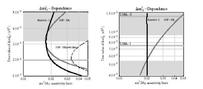
Figure 6: The $\sin^{2}2\theta_{13}$ sensitivity limit as function of the atmospheric (left) and solar (right) mass squared differences for the JPARC-SK (black curves) and Reactor-I (gray curves) experiments from References [29, 30] (five years of neutrino running for JPARC-SK and an integrated luminosity for Reactor-I of $400\,\mathrm{t\,GW\,y}$). In addition, JPARC-SK$@443\,\mathrm{km}$ is shown for a modified baseline of $1.5\times 295\,\mathrm{km}\simeq 443\,\mathrm{km}$ in the left-hand plot (dashed curve). For the oscillation parameters, $\Delta m_{31}^{2}=2.0\cdot 10^{-3}\,\mathrm{eV}^{2}$, $\sin^{2}2\theta_{23}=1.0$, $\Delta m_{21}^{2}=7.5\cdot 10^{-5}\,\mathrm{eV}^{2}$, and $\sin^{2}2\theta_{12}=0.8$ are used (if not varied) [31, 1]. Furthermore, the $3\sigma$ excluded regions are gray shaded and the current best-fit values are marked. The analysis includes systematics, multi-parameter correlations, and degeneracies as in Refs. [32, 30].

The dependence on the true values of the atmospheric and solar mass squared differences is, for the current best-fit values and ranges, illustrated in Figure 6. The figure compares a reactor experiment with an integrated luminosity of $400\,\mathrm{t\,GW\,y}$ to the JPARC to Super-Kamiokande first-generation superbeam experiment with a running time of five years (neutrino running only). The two plots illustrate that the considered reactor experiment would be better than the JPARC-SK superbeam at the current best-fit values of $\Delta m_{31}^{2}$ and $\Delta m_{21}^{2}$, as well as in most of the still allowed parameter ranges. Since the energy spectrum of a reactor experiment is broader than the one of an off-axis (narrow band) superbeam, the reactor experiment is less affected by the smaller value of $\Delta m_{31}^{2}$ after the Super-Kamiokande re-analysis [33]. In addition, it is hardly affected by the true value of $\Delta m_{21}^{2}$ as we discussed above. In the left plot of Figure 6, we also show the JPARC-SK experiment for the (artificial) baseline of $1.5\times 295\,\mathrm{km}\simeq 443\,\mathrm{km}$, which means that for this baseline the oscillation peak is shifted to $\Delta m_{31}^{2}=2.0\cdot 10^{-3}\,\mathrm{eV}^{2}$. The figure clearly demonstrates that this shifting would not solve the problem due to the $1/L^{2}$ luminosity scaling. Because of the over-proportional loss of events for a lower neutrino energy due to the production mechanism and the cross section energy dependence, a lower energy instead of the longer baseline would also not help.

We have now demonstrated that the reactor measurement could provide a more robust limit on $\sin^{2}2\theta_{13}$ with respect to the (within certain ranges) true parameter values of $\Delta m_{31}^{2}$ and $\Delta m_{21}^{2}$. However, it is obvious from Equation (9) that reactor experiments at a baseline of a few kilometers are not sensitive to the mass hierarchy or $\delta_{\mathrm{CP}}$, which means that superbeams will still be needed to test these parameters. On the other hand, a large reactor experiment could help to resolve the degeneracies in Equation (10) by measuring $\sin^{2}2\theta_{13}$. In this case, one could talk about synergies between a reactor experiment and a superbeam. For example, it has been demonstrated in Reference [30] that there are several advantages from a large reactor experiment (e.g., with an integrated luminosity of $8000\,\mathrm{t\,GW\,y}$). First of all, a reactor experiment could help to determine the mass hierarchy very well independently of the true value of $\Delta m_{21}^{2}$. Secondly it could improve the CP sensitivity by allowing to operate the superbeam with neutrinos only (instead of using a fraction of antineutrino running). A reactor experiment performed on a shorter timescale than a superbeam would change the main goal of a superbeam from finding a non-zero value for $\sin^{2}2\theta_{13}$ to measuring $\delta$ and the sign of $\Delta m_{21}^{2}$.

2.5 Theoretical Motivation for non-zero $\theta_{13}$

One may ask if there exist theoretical reasons why $\theta_{13}$ should be within the reach of a new experiment, with a sensitivity down to $\sin^{2}2\theta_{13}\simeq 0.01$. This question is of course connected to the origin of neutrino masses. For example, there exist apparent regularities in the fermionic field content which make it very tempting to introduce right-handed neutrino fields leading to both Dirac and Majorana mass terms for neutrinos. The diagonalization of the resulting mass matrices yields Majorana mass eigenstates and generically very small neutrino masses. This is the well known see-saw mechanism [34]. It can be nicely accommodated in embeddings of the SM into a larger gauge symmetry, such as SO(10).

A reason for expecting a particular value of $\theta_{13}$ does clearly not exist as long as one extends the SM only minimally to accommodate neutrino masses. $\theta_{13}$ is then simply some unknown parameter which could take an arbitrarily small value, including zero. The situation changes in models of neutrino masses. Even then one should acknowledge that in principle any value of $\theta_{13}$ can be accommodated. Indeed, before the discovery of large leptonic mixing, many theorists who did consider lepton mixing expected it to be similar to quark mixing, characterized by small mixing angles. Experiment led theory in showing the striking results that $\sin^{2}2\theta_{23}\simeq 1$ and $\tan^{2}\theta_{12}\simeq 0.44$, while $\theta_{13}$ is small. Indeed, the most remarkable property of leptonic mixing is that two angles are large. Therefore, today there is no particular reason to expect the third angle, $\theta_{13}$, to be extremely small or even zero. This can be seen in neutrino mass models which are able to predict a large $\theta_{12}$ and $\theta_{23}$. They often have a tendency to predict also a sizable value of $\theta_{13}$. This is both the case for models in the framework of Grand Unified Theories and for models using flavor symmetries. There exist also many different texture models of neutrino masses and mixings, which accommodate existing data and try to predict the missing information by assuming certain elements of the mass matrix to be either zero or equal. Again one finds typically a value for $\theta_{13}$ which is not too far from current experimental bounds. A similar behavior is found in so-called “anarchic mass matrices”. Starting essentially with random neutrino mass matrix elements one finds that large mixings are actually quite natural.

An overview of various predictions is given in Table 1. For more extensive reviews, see for example [35, 36, 37, 38]. The conclusion from all these considerations about neutrino mass models is that a value of $\theta_{13}$ close to the CHOOZ bound would be quite natural, while smaller values become harder and harder to understand as the limit on $\theta_{13}$ is improved.

Reference	$\sin\theta_{13}$	$\sin^{2}2\theta_{13}$
SO(10)
Goh, Mohapatra, Ng [40]	0.18	0.13
Orbifold SO(10)
Asaka, Buchmüller, Covi [41]	0.1	0.04
SO(10) + flavor symmetry
Babu, Pati, Wilczek [42]	$5.5\cdot 10^{-4}$	$1.2\cdot 10^{-6}$
Blazek, Raby, Tobe [43]	0.05	0.01
Kitano, Mimura [44]	0.22	0.18
Albright, Barr [45]	0.014	$7.8\cdot 10^{-4}$
Maekawa [46]	0.22	0.18
Ross, Velasco-Sevilla [47]	0.07	0.02
Chen, Mahanthappa [48]	0.15	0.09
Raby [49]	0.1	0.04
SO(10) + texture
Buchmüller, Wyler [50]	0.1	0.04
Bando, Obara [51]	0.01 .. 0.06	$4\cdot 10^{-4}$ .. 0.01
Flavor symmetries
Grimus, Lavoura [52, 53]	0	0
Grimus, Lavoura [52]	0.3	0.3
Babu, Ma, Valle [54]	0.14	0.08
Kuchimanchi, Mohapatra [55]	0.08 .. 0.4	0.03 .. 0.5
Ohlsson, Seidl [56]	0.07 .. 0.14	0.02 .. 0.08
King, Ross [57]	0.2	0.15
Textures
Honda, Kaneko, Tanimoto [58]	0.08 .. 0.20	0.03 .. 0.15
Lebed, Martin [59]	0.1	0.04
Bando, Kaneko, Obara, Tanimoto [60]	0.01 .. 0.05	$4\cdot 10^{-4}$ .. 0.01
Ibarra, Ross [61]	0.2	0.15
$3\times 2$ see-saw
Appelquist, Piai, Shrock [62, 63]	0.05	0.01
Frampton, Glashow, Yanagida [64]	0.1	0.04
Mei, Xing [65] (normal hierarchy)	0.07	0.02
Mei, Xing [65] (inverted hierarchy)	$>0.006$	$>1.6\cdot 10^{-4}$
Anarchy
de Gouvêa, Murayama [66]	$>0.1$	$>0.04$
Renormalization group enhancement
Mohapatra, Parida, Rajasekaran [67]	0.08 .. 0.1	0.03 .. 0.04

Table 1: Incomplete selection of predictions for $\theta_{13}$. The numbers should be considered as order of magnitude statements.

Besides, neutrino masses and mixing parameters are subject to quantum corrections between low scales, where measurements are performed, and high scales where some theory predicts $\theta_{13}$. Even in the “worst case” scenario, where $\theta_{13}$ is predicted to be exactly zero, they cause $\theta_{13}$ to run to a finite value at low energy. Strictly speaking, $\theta_{13}=0$ cannot be excluded completely by this argument, as the high-energy value could be just as large as the change due to running and of opposite sign. However, a severe cancellation of this kind would be unnatural, since the physics generating the value at high energy are not related to those responsible for the quantum corrections. The strength of the running of $\theta_{13}$ depends on the neutrino mass spectrum and whether or not supersymmetry is realized. For the Minimal Supersymmetric Standard Model one finds a shift $\Delta\sin^{2}2\theta_{13}>0.01$ for a considerable parameter range, i.e. one would expect to measure a finite value of $\theta_{13}$ [39]. Conversely, limits on model parameters would be obtained if an experiment were to set an upper bound on $\sin^{2}2\theta_{13}$ in the range of 0.01. In any case, it should be clear that a precision of the order of quantum corrections to neutrino masses and mixings is very interesting in a number of ways.

Altogether there exist very good reasons to push the sensitivity limit from the current CHOOZ value by an order of magnitude and to hope that a finite value of $\theta_{13}$ will be found. But as already mentioned, at this precision even a negative result would be very interesting, since it would test or rule out many neutrino mass models and restrict parameters relevant for quantum corrections to masses and mixings. From a larger point of view the experiments discussed in this white paper might probe if a small value of $\theta_{13}$ is a numerical coincidence or the result of some underlying symmetry.

3 Optimal Baseline Distances, Luminosity Scaling, and the Impact of Systematics

3.1 Total Flux vs. Baseline

The equation for the survival probability of reactor neutrinos under full three flavor mixing was previously described in Equation (2). It was pointed out by reference to Figure 3 that a judicious choice of baseline distance could restrict one to oscillations dominated by one or the other of the $\Delta m^{2}$ oscillations. For this experiment, we are choosing to focus on the shorter baseline, which corresponds to $\Delta m^{2}_{atm}$. Thus, neglecting the other oscillation term, Equation (2) reduces to

$$P(\bar{\nu}_{e}\rightarrow\bar{\nu}_{e})=1-\sin^{2}(2\theta_{13})\sin^{2}(\Delta m^{2}_{atm}L/4E)$$ (11)

where the current best estimate from Super-Kamiokande has $\Delta m^{2}_{atm}=0.002$ [33]. To measure this oscillation effect, the optimal choice in baseline distance will depend on the energy of the neutrinos. As shown previously in Figure 5, the detected spectrum for reactor neutrinos is between 1-10 MeV with a peak at about 3.8 MeV. In addition, recall that the flux of neutrinos will fall as the square of the baseline distance.

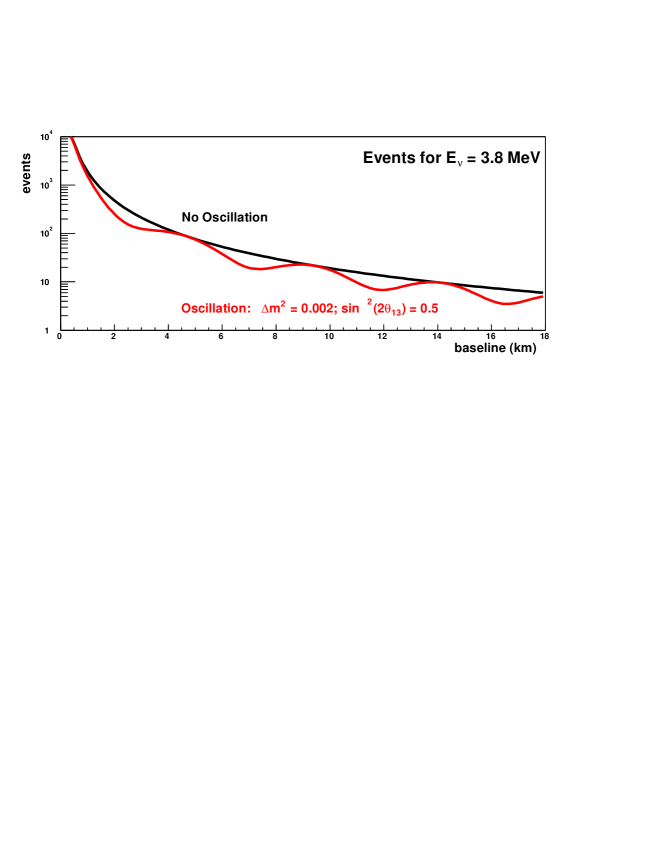
Figure 7: Illustrative expected number of detected neutrino events as a function of baseline distance from the reactor core. The two curves show the expectations for the case of no oscillations and for an oscillation with $\Delta m^{2}=0.002$ and an amplitude of $\sin^{2}(2\theta_{13})=0.5$ which is 2.5 times the current limit. The curves are calculated for a luminosity of $\mathrm{600\,t\,GW\,y}$ and a mono-energetic neutrino flux at 3.8 MeV.

A comparison of the expected flux with and without oscillations is shown in Figure 7 for a mono-energetic neutrino beam of 3.8 MeV. Note that the amplitude of the oscillation shown is set to $\sin^{2}(2\theta_{13})=0.5$ which is 2.5 times the current limit from CHOOZ in order to amplify the effect. As would be expected, one sees the disappearance effect at regular intervals. However, when the full energy spectrum, shown in Figure 5, is folded in, the regular disappearance effect is washed out even with the magnified amplitude (see Figure 8).

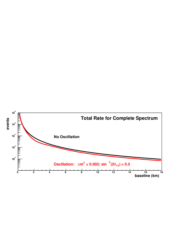
Figure 8: Expected number of detected neutrino events as a function of baseline distance from the reactor core. The two curves show the expectations for the case of no oscillations and for an oscillation with $\Delta m^{2}=0.002$ and an amplitude of $\sin^{2}(2\theta_{13})=0.5$ which is 2.5 times the current limit. The curves are calculated using the complete energy spectrum from a nuclear reactor and a luminosity of $\mathrm{600\,t\,GW\,y}$.

In order to make the oscillation effect in Figure 8 visible, the ratio of the two curves is shown in Figure 9.

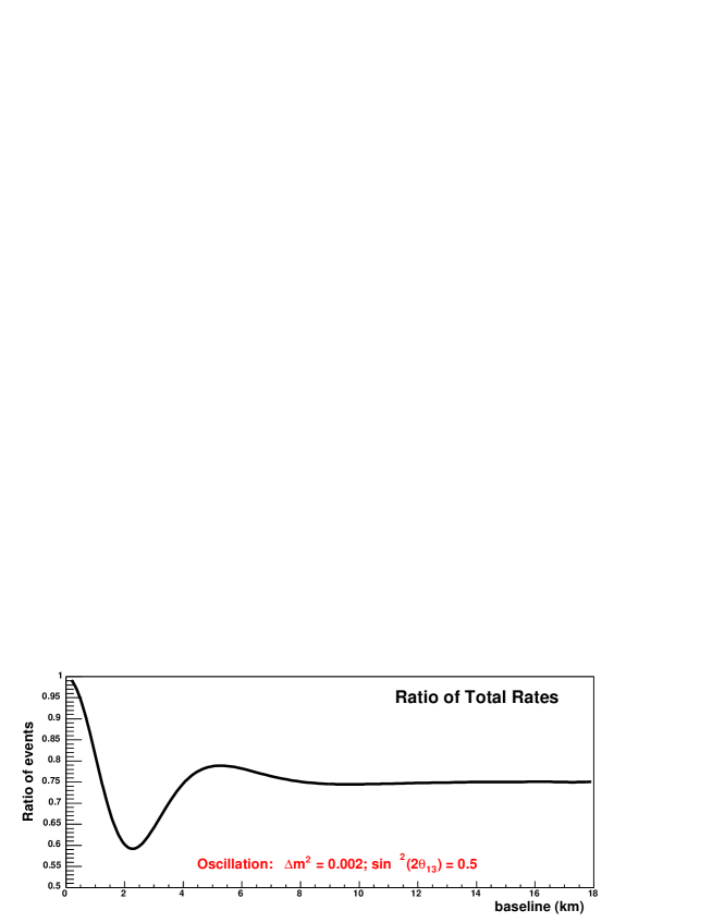
Figure 9: The ratio of the expected number of neutrino events with and without oscillations as a function of distance from the reactor core. This calculation was made for a luminosity of $\mathrm{600\,t\,GW\,y}$ and includes the true neutrino energy spectrum. The oscillation is assumed to have $\Delta m^{2}=0.002$ and an amplitude of $\sin^{2}(2\theta_{13})=0.5$ which is 2.5 times the current allowed limit.

Notice that the largest deviation occurs at a baseline distance of just over 2 kilometers. This corresponds to the first oscillation for $E_{\nu}=3.8$ MeV as shown in Figure 7. This makes sense since this is the peak of the neutrino energy spectrum and therefore has the most statistical power. However, it is clear that as baseline distance increases, the effect of other parts of the energy spectrum being at their respective maxima and minima of oscillation effectively neutralizes any ability to detect a specific oscillation signature.

3.2 Spectral Shape Information

From Equation (11), it is clear that neutrinos of differing energies oscillate with different frequencies. Figure 9 shows that observable oscillation effects in the total number of neutrinos detected wash out with increasing baseline distance. But by looking at the specific energy distribution of the detected neutrinos, more information is available.

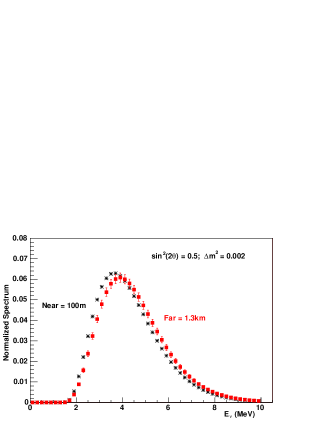
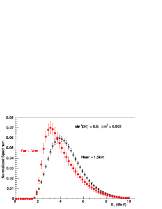
Figure 10: Comparisons of the expected measured neutrino energy spectra at various baseline distances in the case of oscillations. The oscillations are assumed to have $\Delta m^{2}=0.002$ and an amplitude of $\sin^{2}(2\theta_{13})=0.5$ which is 2.5 times the current limit in order to magnify the effect. These plots show the expected statistics for a luminosity of $\mathrm{600\,t\,GW\,y}$ at the specified baseline distance.

In Figure 10, two comparisons of the normalized energy spectra are shown. These plots show statistical errors only for 0.2 MeV bins and a luminosity of $\mathrm{600\,t\,GW\,y}$ at each location. As with the previous plots, the amplitude of the oscillation has been magnified by a factor of 2.5 ($\sin^{2}(2\theta_{13})=0.5$) and a mass difference of $\Delta m^{2}=0.002$ has been used. In addition, an energy resolution of 10%/$\sqrt{E}$ has been assumed. The plot on the left compares the spectrum at 100 meters, which is effectively unoscillated, with the spectrum at 1.3 kilometers. One can notice that at this distance, the low energy part of the spectrum is showing a deficit with respect to the near detector spectrum. However, one could also confuse this with an overall shift in the absolute energy scale between the two detector locations.

The right plot of Figure 10, however, compares two oscillated spectra from 1.5 and 3 kilometers. Notice that the shapes of the spectra are vastly different. This arises from the fact that at 3 kilometers it is the high energy part of the spectrum which is fully oscillated away while the low energy part has returned to full presence. It is interesting to note that the statistical significance of the spectral distortions in the two plots is nearly identical. While the total number of events is significantly higher in the plot with baselines of 100 m and 1.3 km, the spectral distortion is much more pronounced in the plot with baselines of 1.5 and 3 km. These two effects appear to compensate one another.

3.3 Combining Shape and Rate Information

It turns out that the most statistically significant spectral shape distortion, given the assumed oscillation parameters above, is achieved for a near detector at the closest possible location and a far detector at about 1 kilometer. Thus the spectral shape information has a different optimal baseline than the depletion of the total flux, which was previously observed to be maximal at just over 2 kilometers from the source.

Since the spectral shape measurement requires the use of a normalized energy spectrum at each location, the statistical significance of each measurement (each bin) is weighted by the total flux at that location. This gives a 1/L² reduction in the statistical sensitivity. Therefore, from a strictly statistical perspective, the total flux measurement will have slightly more than a factor of two more power. However, the total flux measurement is susceptible to systematic differences between the two detectors. Since the normalized energy spectra are normalized to the total number of events at that location, all systematic effects, except those which will be uncorrelated bin-to-bin within a detector, will be removed. This additional freedom from systematic effects implies that in the limit of infinite statistics, a more precise measurement can be made with the information from the energy spectrum.

This interplay between the two methods can be seen graphically by referring to the plot in Figure 11 (see also the discussion in Sec. 3.4). There, the sensitivity to $\sin^{2}(2\theta_{13})$ is shown as a function of luminosity. At low luminosity ($\cal L<\mathrm{400t\,GW\,y}$) the sensitivity is directly proportional to statistics and is dominated by the total flux measurement. Then, for luminosities between $\mathrm{400}$ and $\mathrm{6000\,t\,GW\,y}$, additional statistics do not make significant gains in the sensitivity. In this region, the systematic uncertainties between the two detectors (called $\sigma_{norm}$ in this plot) become dominant. However, beyond $\mathrm{6000\,t\,GW\,y}$, notice that the sensitivity again becomes proportional to the statistics. This is caused by the fact that enough statistics have been gained to allow the spectral measurements to dominate over the systematically limited flux measurement.

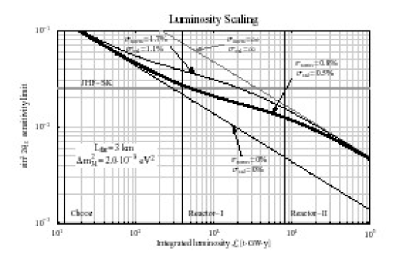
Figure 11: The sensitivity to $\sin^{2}2\theta_{13}$ at 90% CL as a function of the integrated luminosity for different values of the normalization error $\sigma_{\mathrm{norm}}$ and the energy calibration error $\sigma_{\mathrm{cal}}$. The vertical lines mark the luminosities of the CHOOZ experiment and our standard setups Reactor-I and Reactor-II. We take $\Delta m^{2}_{31}=2\times 10^{-3}$ eV² and $L_{FD}=3$ km.The horizontal line shows a typical sensitivity limit obtainable by the JHF-SK superbeam experiment (also known as JPARC-$\nu$) for the same parameter values.

Realization of this interplay between the methods implies that the optimal choice of baseline distance depends on the expected luminosity of the experiment. Since most of the discussion in this paper does not expect a luminosity of greater than $\mathrm{6000\,t\,GW\,y}$ (which would require kiloton sized detectors), we will focus on measurements in which the total flux measurement is not systematically limited. To make optimal use of the available statistics, we therefore wish to combine the information from the total flux and energy spectral measurements at both detectors. One can rather simply create a chi-squared comparison of the two statistical distributions which takes into account both sets of information with the following definition:

$$\chi^{2}=\sum_{i}\frac{\left[N^{far}_{i}-\left(\frac{L_{near}}{L_{far}}\right)^{2}N^{near}_{i}\right]^{2}}{\left[N^{far}_{i}+\left(\frac{L_{near}}{L_{far}}\right)^{4}N^{near}_{i}\right]}$$ (12)

where $L$ refers to the baseline distance to the near or far detectors and $N_{i}$ refers to the number of events in the $i$-th bin of the measured energy spectrum at that detector. By using the definition of Equation (12), one can determine the 90% confidence level limit on a measurement of $\sin^{2}(2\theta_{13})$ for a given luminosity. This is shown as a function of baseline distance in Figure 12 assuming a luminosity of $\mathrm{600\,t\,GW\,y}$. For this estimation, the near detector is assumed to be fixed at 300 meters and a 1% systematic limit has been used.

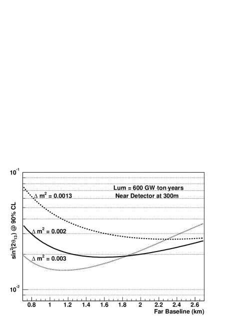
Figure 12: Statistical sensitivity to $\sin^{2}(2\theta_{13})$ as a function of baseline distance to the far detector. The statistical power is calculated using Equation (12) with a luminosity of $\mathrm{600\,t\,GW\,y}$ and a 1% systematic limit bin-to-bin. Curves are shown for three values of $\Delta m^{2}$ representing the best fit and the upper and lower limits of the 90% allowed region from the Super-Kamiokande experiment.

One can see that for the current best fit value of $\Delta m^{2}=0.002$, the optimal baseline distance for the far detector is at 1.6 kilometers. However, given that the optimal distance depends quite strongly on the value of $\Delta m^{2}$, we also show the sensitivity plots for values of $\Delta m^{2}$ which match the upper and lower bounds of the 90% allowed region from Super-Kamiokande. Notice that for each curve, the sensitivity to $\sin^{2}(2\theta_{13})$ is relatively flat around the optimum. Therefore, a reasonable sensitivity can be reached, with flexibility to various values of $\Delta m^{2}$, for a far detector baseline distance between 1.2 and 2.4 kilometers.

3.4 Statistical Analysis and Luminosity Scaling

In this section some general analysis methods are proposed to investigate the sensitivity to $\theta_{13}$ in a reactor experiment with two detectors and one single reactor. The impact of the integrated luminosity, positions of the near detector, various systematic errors, and a possible background on the sensitivity limit are discussed. As a measure for the “size” of the experiment the integrated luminosity $\mathcal{L}$ is useful, which is defined as $\mathcal{L}$ = fiducial detector mass [tons] $\times$ thermal reactor power [GW] $\times$ running time [years] (assuming 100% detection efficiency and no deadtimes). We define two benchmark setups Reactor-I ($\mathcal{L}=400$ t GW y) and Reactor-II ($\mathcal{L}=8000$ t GW y) corresponding roughly to 31 500 and 630 000 reactor neutrino events for no oscillations, respectively, assuming a PXE-based scintillator.

We take into account that spectral information is available in the near, as well as in the far detector in form of $N_{\mathrm{bins}}$ bins in positron energy. For the theoretical prediction for the number of reactor neutrino events in the $i$th energy bin of the near ($A=N$) and far ($A=F$) detector, respectively, we write

$$T^{A}_{i}=(1+a+b^{A}+c_{i})N_{i}^{A}+g^{A}M_{i}^{A}\,,$$ (13)

and consider a $\chi^{2}$-function including the full spectral information from both detectors:

$$\chi^{2} = \sum_{i=1}^{N_{\mathrm{bins}}}\left[\sum_{A=N,F}\frac{(T_{i}^{A}-O_{i}^{A})^{2}}{O_{i}^{A}+\sigma_{\mathrm{exp}}^{2}(O_{i}^{A})^{2}+B_{i}^{A}+\sigma_{\mathrm{BG}}^{2}(B_{i}^{A})^{2}}+\left(\frac{c_{i}}{\sigma_{\mathrm{shape}}}\right)^{2}\right]$$ (14)

$$+ \sum_{A=N,F}\left[\left(\frac{b^{A}}{\sigma_{b}}\right)^{2}+\left(\frac{g^{A}}{\sigma_{\mathrm{cal}}}\right)^{2}\right]+\left(\frac{a}{\sigma_{a}}\right)^{2}\,.$$

Here, $N_{i}^{A}$ is the expected number of events in the $i$th energy bin of the corresponding detector, which depends on the oscillation parameters. $N_{i}^{A}$ is calculated by folding the reactor neutrino spectrum, the detection cross section for inverse beta decay, the $\bar{\nu}_{e}$ survival probability, and the energy resolution function. In the numerical calculations we assume an energy resolution of $5\%/\sqrt{E_{\mathrm{vis}}[\mathrm{MeV}]}$, and we use $62$ bins in the range between $E_{\bar{\nu}_{e}}=1.8\,\mathrm{MeV}$ and $E_{\bar{\nu}_{e}}=8.0\,\mathrm{MeV}$, corresponding to a bin width of $0.1\,\mathrm{MeV}$. $O_{i}^{A}$ is the observed number of events. In the absence of real data, we take for $O_{i}^{A}$ the expected number of events for some fixed “true values” of the oscillation parameters, e.g., to calculate a sensitivity limit the expected number of events for $\theta_{13}=0$ is used. If the near detector is so close to the reactor that no oscillations will occur, the $T_{i}^{N}$ will not depend on the oscillation parameters, and in that case one can set $O_{i}^{N}=N_{i}^{N}$. The quantities $T_{i}^{A}$ and $O_{i}^{A}$ correspond only to reactor neutrino events. If a certain background has to be subtracted from the actual number of events it will contribute to the statistical and systematic errors. In Equation (14) $B_{i}^{A}$ is the number of background events in the $i$th bin of detector $A$, and we assume that it is known with an (uncorrelated) error $\sigma_{\mathrm{BG}}$.

For each point in the space of oscillation parameters, the $\chi^{2}$-function has to be minimized with respect to the parameters $a,b^{N}$, $b^{F}$, $g^{N}$, $g^{F}$, and $c_{i}$ modeling various systematic errors.

1. The parameter $a$ refers to the error on the overall normalization of the number of events common to near and far detectors, and $\sigma_{a}$ is typically of the order of a few percent. The main source for such an error is the uncertainty of the neutrino flux normalization.

2. The parameters $b^{N}$ and $b^{F}$ parameterize the uncorrelated normalization uncertainties of the two detectors. Here contributes, for instance, the error on the fiducial mass of each detector. We assume that in this case an error below 1% can be reached.

3. The energy scale uncertainty in the two detectors is taken into account by the parameters $g^{N}$ and $g^{F}$. To this aim we replace in $N_{i}^{A}$ the visible energy $E_{\mathrm{vis}}$ by $(1+g^{A})E_{\mathrm{vis}}$, and to first order in $g^{A}$ we have $N_{i}^{A}(g^{A})\approx N_{i}^{A}(g^{A}=0)+g^{A}\,M_{i}^{A}$. A typical value for this error on the energy calibration is $\sigma_{\mathrm{cal}}\sim 0.5\%$.

4. In order to model an uncertainty on the shape of the expected energy spectrum, we introduce a parameter $c_{i}$ for each energy bin, known with an error $\sigma_{\mathrm{shape}}$. This corresponds to a completely uncorrelated error between different energy bins, which is the most pessimistic assumption of no knowledge of possible shape distortions. However, we choose this error fully correlated between the corresponding bins in the near and far detector (the same coefficient is used for the corresponding bins in the two detectors), since shape distortions should affect the signals in both detectors of equal technology in the same way.

5. We include the possibility of an uncorrelated experimental systematic error $\sigma_{\mathrm{exp}}$. In this way we assume that the observed number of events in each bin and each detector $O_{i}^{A}$ has in addition to the statistical error $\pm\sqrt{O_{i}^{A}}$ the (uncorrelated) systematic error $\pm\sigma_{\mathrm{exp}}O_{i}^{A}$. We call this uncertainty “bin-to-bin error”. Taking it completely uncorrelated between energy bins as well as between the near and far detectors corresponds again to the worst case scenario. Values of $\sigma_{\mathrm{exp}}$ at the per mil level should be realistic.

Note that all the parameters describing the systematic errors are at most at the percent level, which means that the linear approximation in Equation (13) is justified. The following discussion of general features of such an analysis is based on the results reported in Reference [30].

Let us first assume that the near detector is close enough to the reactor, such that no oscillations develop ($L_{ND}\lesssim 200$ m). Furthermore, we first assume that the background is negligible, and $\sigma_{\mathrm{exp}}\lesssim 0.1\%$ and $\sigma_{\mathrm{shape}}\lesssim 2\%$, which means that these errors can be neglected. Then the $\chi^{2}$-analysis can be significantly simplified. In particular, it is not necessary to explicitly include the near detector in the analysis and Equation (14) becomes [30]

$$\chi^{2}_{F}=\sum_{i}\frac{(T_{i}^{F}-O_{i}^{F})^{2}}{O_{i}^{F}}+\left(\frac{g^{F}}{\sigma_{\mathrm{cal}}}\right)^{2}+\left(\frac{\alpha}{\sigma_{\mathrm{norm}}}\right)^{2}$$ (15)

with

$$\sigma_{\mathrm{norm}}^{2}=\bar{\sigma}^{2}+\sigma_{b}^{2}\,,\qquad\frac{1}{\bar{\sigma}^{2}}\approx\frac{1}{\sigma_{a}^{2}}+\frac{1}{\sigma_{b}^{2}}\,.$$ (16)

For example, assuming typical values of $\sigma_{a}=2\%$ for the flux uncertainty and $\sigma_{b}=0.6\%$ for the detector-specific uncertainty, we obtain with Equation (16) an effective normalization error of $\sigma_{\mathrm{norm}}\simeq 0.8\%$. This is the value which is used for the numerical calculations.

In Figure 11, we show the sensitivity to $\sin^{2}2\theta_{13}$ as a function of the integrated luminosity ${\cal L}$. In this figure, the lower diagonal curve corresponds to the idealized case of statistical errors only, and shows just the expected $1/\sqrt{\cal L}$ scaling, whereas the values $\sigma_{\mathrm{norm}}=0.8\%$ and $\sigma_{\mathrm{cal}}=0.5\%$ lead to the thick curve. At a luminosity around $100\,\mathrm{t\,GW\,y}$, we detect a departure from the statistics dominated regime into a flatter systematics dominated region. This effect is dominated by the error on the normalization $\sigma_{\mathrm{norm}}$, whereas the energy calibration error $\sigma_{\mathrm{cal}}$ only plays a minor role. In fact, we find that for all considered cases (including Reactor-I and Reactor-II) the impact of the energy scale uncertainty is very small, as long as the oscillation minimum is well inside the observable energy spectrum. Hence, we will neglect this error in the following.

At large luminosities $\gtrsim 10^{4}\,\mathrm{t\,GW\,y}$, the slope of the curve changes, and we are entering again a statistics dominated region with a $1/\sqrt{\cal L}$ scaling. This interesting behavior can be understood as follows. For low luminosities the sensitivity to $\sin^{2}2\theta_{13}$ comes mainly for the total number of events, hence the absolute normalization is important. The turnover of the sensitivity line into the second statistics dominated region occurs at the point where the spectral shape distortion becomes more important than the total rate, which implies that the overall normalization, and consequently also the actual value of $\sigma_{\mathrm{norm}}$, becomes irrelevant. We illustrate this by the upper thin black line, which shows the luminosity scaling for the case of larger systematic errors. As an example, we choose values of $\sigma_{\mathrm{norm}}=1.7\%$ for the normalization and $\sigma_{\mathrm{cal}}=1.1\%$ for the energy calibration. We find that, in this case, the transition to the systematics dominated regime occurs at much smaller luminosities. However, for large luminosities, the same limit is approached as for the more optimistic case. The diagonal gray curve shows the limit for no constraint at all on the normalization and energy calibration. Even in this extreme case, we obtain the same limit for high luminosities.

Figure 13: Sensitivity to $\sin^{2}2\theta_{13}$ at 90% CL as a function of the luminosity for an uncorrelated experimental systematic error (“bin-to-bin error”) $\sigma_{\mathrm{exp}}=0.1\%$ and 0.5%, and background levels in the far detector relative to the total number of events for no oscillations of 1% and 5%. Here $L_{ND}=0.2$ km, $L_{FD}=1.7$ km, $\Delta m^{2}_{31}=2\times 10^{-3}$ eV², and $\sigma_{\mathrm{shape}}=2\%$. Identical detector masses are assumed for near and far detectors.

3.5 Systematics, Background, and the Position of the Near Detector

In the following we investigate the impact of various systematic effects beyond the simple overall normalization. To this end we apply the full $\chi^{2}$ function as given in Equation (14). In Figure 13 the luminosity scaling of the $\sin^{2}2\theta_{13}$-limit is shown for various choices for the experimental bin-to-bin error $\sigma_{\mathrm{exp}}$ (see item 5 above) and background levels in the far detector. For the sake of concreteness we assume a flat background in each detector $B_{i}^{A}=B^{A}$ with an error of $\sigma_{\mathrm{BG}}=10\%$. The size of the backround is measured by $f_{\mathrm{BG}}$, which is defined as the fraction of the total number of background events relative to the total number of reactor neutrino events for no oscillations, i.e., $B^{A}=f_{\mathrm{BG}}\sum_{i}N^{A}_{i,\mathrm{no\,osc}}/N_{\mathrm{bins}}$. From the figure we find that Reactor-I is not affected by a bin-to-bin error up to 0.5%, nor by backgrounds in the far detector up to 5%. In contrast, such errors and backgrounds are important to some extent for big experiments like Reactor-II. In that case values of $\sigma_{\mathrm{exp}}\gtrsim 0.1\%$ start to deteriorate the sensitivity limit, and the background in the far detector should be smaller than 1% of the reactor neutrino signal. We note that backgrounds in the near detector up to a few percent do not affect the result. Regarding the huge number of reactor neutrino events in the near detector it should be possible to obtain backgrounds below 1%.

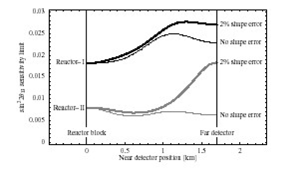
Figure 14: The sensitivity to $\sin^{2}2\theta_{13}$ at the 90% CL for Reactor-I and Reactor-II as a function of the near detector position. The far detector is situated at 1.7 km and we assume identical detector masses and $\Delta m^{2}_{31}=3\times 10^{-3}$ eV². Furthermore, the impact of an uncorrelated theoretical shape uncertainty $\sigma_{\mathrm{shape}}=2\%$ is shown.

For practical reasons it might be hard to find a reactor station where a near detector can be situated very close ($\lesssim 200\,\mathrm{m}$) to the core with sufficient rock overburden. Therefore, it is interesting to investigate the impact of larger near detector baselines on the $\sin^{2}2\theta_{13}$ limit. In this case the information provided by the near detector on the initial flux normalization and energy shape is already mixed with some oscillation signature. The results of such an analysis are presented in Figure 14. We find that for the case of Reactor-I the limit starts deteriorating around a near detector distance of 400 m, whereas for Reactor-II the limit even improves slightly up to near detector baselines of $\sim 1\,\mathrm{km}$. Due to the high statistics in the case of Reactor-II, flux normalization and shape are very well determined by the near detector even in the presence of some effect of $\theta_{13}$, and the additional information on oscillations improves the limit a bit. Furthermore, we find from Figure 14 that the shape uncertainty becomes important for near detector baselines $\gtrsim 1.1\,\mathrm{km}$, especially for Reactor-II. A reduction of this theoretical error would be helpful in such a situation. We note that assuming the shape error to be completely uncorrelated corresponds to the worst case. A more realistic implementation of the shape uncertainty including correct correlations will lead to results somewhere in between the curves for no and 2% shape error in Figure 14. We have verified that for Reactor-I the worsening of the limit comes mainly from the fact that with increasing near detector baselines the number of events decreases rapidly, i.e., it is statistics dominated, whereas for Reactor-II the loss in sensitivity is driven by the systematic shape uncertainty and cannot be compensated by larger near detectors.

		Reactor-I	Reactor-II
Effective normalization	$\sigma_{\mathrm{norm}}=0.8\%$	important	not important
Energy calibration	$\sigma_{\mathrm{cal}}\simeq 0.5\%$	not important	not important
Exp. bin-to-bin uncorr. error	$\sigma_{\mathrm{exp}}\lesssim 0.1\%$	not important	important
background in far detector	$f_{\mathrm{BG}}\lesssim 1\%$	not important	important
near detector baseline		$L_{ND}\lesssim 400$ m	$L_{ND}\lesssim 1$ km
theor. shape uncertainty	$\sigma_{\mathrm{shape}}=2\%$	important for $L_{ND}\gtrsim 1$ km

Table 2: Relevance of various systematic errors for the two reactor benchmark setups Reactor-I and Reactor-II.

To summarize, for the case of the Reactor-I setup (400 t GW y) the main information comes from the total number of events and the systematic normalization error dominates. In order to obtain a reliable limit, it should therefore be well under control. For large luminosities, such as for the Reactor-II setup (8000 t GW y), the sensitivity limit comes mainly from spectral shape information and is independent of normalization errors. In that case a bin-to-bin uncorrelated experimental systematic error should be below 0.1% and the background should be at the 1% level. Furthermore, for the case of Reactor-I-like experiments one should look for a site where the near detector can be placed at a distance of at most 400 m from the reactor. For large detectors, such as Reactor-II, near detector baselines of up to 1 km will perform well. For near detector baselines longer than about 1 km the correct treatment of the theoretical shape uncertainty becomes important. These results are summarized in Table 2.

4 Previous Reactor Experiments

Here we review the three most recent previous neutrino experiments at reactors. The best current limit on $\theta_{13}$ comes from CHOOZ. An experiment with similar distance and running time, but smaller overburden, was conducted at Palo Verde. Finally the KamLAND experiment was conducted with much larger overburden, and larger size, but much longer baseline, which resulted in a reduced sensitivity to $\theta_{13}$ but unprecedented sensitivity to $\theta_{12}$. These previous experiments are reviewed in order to present several lessons which are needed to show that a future experiment can control systematics to the level below one percent.

4.1 CHOOZ

The CHOOZ experiment [10, 11, 69] was located close to the Chooz nuclear power plant, in the North of France, 10 km from the Belgian border. The power plant consists of two twin pressurized water reactors (PWR), the first of a series of the newly developed PWR generation in France. The thermal power of each reactor is 4.25 GW (1.3 GW electrical). These reactors started respectively in May and August 1997, just after the start of the data taking of the CHOOZ detector (April 1997). This opportunity allowed a measurement of the reactor-OFF background and a separation of individual reactor’s contributions.

The detector was located in an underground laboratory about 1 km from the neutrino source. The 300 mwe rock overburden reduced the external cosmic ray muon flux, by a factor about 300, to a value of $0.4\,$m${}^{-2}\,s^{-1}$. This was the main criterion to choose this site. Indeed, the previous experiment at the Bugey reactor power plant showed the necessity of reducing by 2 orders of magnitude the flux of fast neutrons produced by muon-induced nuclear spallations in the material surrounding the detector. The neutron flux in CHOOZ was measured at energies larger than 8 MeV (endpoint of the neutrino flux from nuclear reactors) and found to be 1/day, in good agreement with expectation.

The detector envelope consisted of a cylindrical steel vessel, 5.5 m in diameter and 5.5 m in height. The vessel was placed in a pit (7 m diameter and 7 m deep), and was surrounded by 75 cm of low activity sand. It was composed of three concentric regions:

• a central 5 ton target in a transparent plexiglass container filled with a 0.09 % Gd-loaded scintillator

• an intermediate 70 cm thick region, filled with non loaded scintillator and used to protect the target from PMT radioactivity and to contain the gamma from neutron capture on Gd. These 2 first regions were viewed by 192 PMTs

• an outer veto, filled with the same scintillator.

The scintillator showed a degradation of the transparency over time, which resulted in a decrease of the light yield (live time around 250 days). The event position was reconstructed by fitting the charge balance, with a typical precision of 10 cm for the positron and 20 cm for the neutron. The time reconstruction was found to be less precise on source and laser tests, due to the small size of the detector. The reconstruction became more difficult when the event was located near the PMTs, due to the $1/r^{2}$ divergence of the light collected (see Figure 31 of [10]).

The final event selection used the following cuts :

• positron energy smaller than 8 MeV (only 0.05 % of the positrons have a bigger energy)

• neutron energy between 6 and 12 MeV

• distance from the PMT surface bigger than 30 cm for both positron and neutron

• distance between positron and neutron smaller than 100 cm

• only one neutron

• time window between positron and neutron signals is from 2 to 100 $\mu$s.

The 6 MeV cut on the gamma ray’s total energy from a neutron capture on Gd cannot be computed from a simulation, because only the global released energy is known. The number of gammas and their individual energies were very poorly known. The scintillating buffer around the target was important to reduce the gamma escape. This cut was calibrated with a neutron source (0.4 % systematic error). The 3 cuts on the distances were rather difficult to calibrate, due to the difficulty of the reconstruction described above. This created a tail of mis-reconstructed events, which was very difficult to simulate (0.4 % systematic error on the positron-neutron distance cut). The positron threshold was carefully calibrated, as shown in Figure 39 of [10]. The value of the threshold depends upon the position of the event, due to the variation of solid angles and to the shadow of some mechanical pieces such as the neck of the detector (0.8 % systematic error). The time cut relied on MC simulation. The time spectrum happened to be exponential to $>20\,\mu$s, but there was no reason for this (the Gamow law, which allows to demonstrate an exponential behavior is wrong for Gd, whose capture cross section is only epithermal). The corresponding systematic error was estimated to be 0.4%.

The final result was given as the ratio of the number of measured events versus the number of expected events, averaged on the energy spectrum. It was:

R = 1.01 $\pm$ 2.8 % (stat) $\pm$ 2.7 % (sys)

Two components were identified in the background :

• a correlated one, which has a flat distribution for energies bigger than 8 MeV, and is due to the recoil protons from fast spallation neutrons. It was extrapolated to 1 event/day.

• an accidental one, which is obtained from the measure of the single rates.

The background was measured while the reactor was off, and by extrapolating the signal versus power straight line (see Figure 49 of [10]). It is in good agreement with the sum of the correlated and accidental components measured as $1.41\pm 0.24$ events per day. These numbers have to be compared to a signal of 26 events/day at full power.

The systematic errors were due mostly to the reactor uncertainties (2 %), to the detector efficiency (1.5 %), and to the normalization of the detector, dominated by the error on the proton number from the H/C ratio in the liquid (0.8 %). The resulting exclusion plot is shown in Figure 58 of [10]. The corresponding limit on $\sin^{2}2\theta$ is 0.14 for $\Delta m^{2}=2.6\times 10^{-3}$eV², and 0.2 for $\Delta m^{2}=2.0\times 10^{-3}$eV². Due to specific source-detector distance of about 1 km, no limit on $\sin^{2}(2\theta)$ can be set for $\Delta m^{2}=0.8\times 10^{-3}$eV², due to the limited distance from the between the cores and the CHOOZ detector.

4.2 Palo Verde

The Palo Verde experiment was motivated by the discovery of the atmospheric neutrino anomaly [70, 71, 72], which could be explained by neutrino oscillations with large mixing angle and a mass–squared difference in the range of $10^{-3}-10^{-2}$ eV². The Palo Verde experiment, together with the CHOOZ experiment [10, 11, 69] with a similar baseline, were able to exclude the $\nu_{\mu}\rightarrow\nu_{\rm e}$ oscillations as the dominant mechanism for the atmospheric neutrino anomaly. While Palo Verde pursued its goal of exploring the then unknown region of small $\Delta m^{2}$, results from Super-Kamiokande [73] were published which favored the $\nu_{\mu}\rightarrow\nu_{\tau}$ oscillation channel over $\nu_{\mu}\rightarrow\nu_{\rm e}$. In this section, we provide a brief description of the Palo Verde experiment and its final results. Details on the experiment can be found in its physics publications [74, 12, 75, 76] and in technical publications cited below.

The Palo Verde experiment was carried out at the Palo Verde Nuclear Generating Station, located about 80 km west of Phoenix, Arizona. The largest nuclear power plant in the Americas, Palo Verde consists of three identical pressurized water reactors with a total thermal power of 11.63 GW. The detector, containing 11.3 tons of liquid scintillator for the neutrino target, was located at a shallow underground site, 890 m from two of the reactors and 750 m from the third. The 32 meter-water-equivalent overburden entirely eliminated any hadronic component of cosmic radiation and reduced the cosmic muon flux. The collaborating institutions on the experiment were the California Institute of Technology, Stanford University, University of Alabama, and Arizona State University. Data were collected from 1998 to 2000.

A schematic view of the detector is shown in Figure 15. The central detector was an 11 $\times$ 6 matrix of cells. Each cell was 9 m long, subdivided into a 740–cm central section filled with Gd–loaded liquid scintillator [77] and an 80–cm section of mineral oil at either end. The cell was viewed at each end by a 5–inch PMT. Surrounding the central detector along the long sides were tanks providing a layer of water shielding 1 m thick. The water and mineral oil shielding sections attenuate gammas and neutrons emitted from the laboratory walls and outer components of the detector, e.g. the glass of the PMTs. The detector was fully enclosed by liquid scintillator detectors used to veto cosmic muons.

Figure 15: Schematic view of the detector and the inverse $\beta$-decay reaction producing a triple coincidence pattern inside the detector.

Electron antineutrinos were detected via inverse beta decay, manifested experimentally as a prompt energy deposit due to the kinetic energy and annihilation energy of the positron followed an average of $\sim$28 $\mu$s later by a gamma cascade of 8 MeV total energy due to capture of the neutron on Gd. The central detector was segmented in order to improve the discrimination between positrons from inverse beta decay and electrons, gammas and recoil protons. The experimental signature required for a positron was an energy deposit in one cell greater than $\sim$1 MeV (kinetic energy of the positron) and energy deposits in adjacent cells consistent with those expected from back–to–back 511 keV annihilation gammas.

The event trigger was based on a so–called triple. For triggering, the anode output of the PMT was split and sent to two sets of discriminators, one set having a threshold corresponding to an energy deposit of $\sim$50 keV (“LO”) in the cell and the other set having a threshold corresponding to $\sim$500 keV (’‘HI”). The discriminator outputs were fed into a fast trigger processor [78] which generated a triple if there was a coincidence between at least 2 LOs and 1 HI in any 5 $\times$ 3 cell submatrix in the detector. The occurrence of a triple initiated digitization of the associated event. Readout was carried out if two triples occur within 450 $\mu$s of each other. Given the proximity in time of the “prompt” and “delayed” part of a candidate event, two banks of Fastbus ADCs and TDCs had to be used for digitization. The trigger rates for triples and correlated triples were approximately 50 Hz and 1 Hz, respectively.

The muon veto hit rate was about 2 kHz. A hit in the veto generated 5 $\mu$s of deadtime for the triple trigger processor. Otherwise, muon hits were only clocked and latched for readout, and the main $\mu$ veto cuts were applied off–line.

Detector calibration for energy and position reconstruction was carried out using $\gamma$ point sources, blue LED’s, and a fiber optic flasher system. The detector simulation program used to estimate the triple trigger efficiencies was tuned and checked against data taken with ${}^{22}\!\rm{Na}$ and ${}^{68}\!\rm{Ge}$ sources for the case of positrons and with a ${}^{252}\!\rm{Cf}$ source and a tagged Am–Be source for the case of neutron capture. Detector stability between calibrations was monitored using the LED’s and fiberoptic flasher system.

The expected $\bar{\nu}_{\rm e}$ flux was calculated from the reactor power and fuel composition. The expected $\bar{\nu}_{\rm e}$ interaction rate in the whole target, both scintillator and the acrylic cells, is plotted in Figure 16 for the case of no oscillation from July 1998 to July 2000. Around 220 interactions per day are expected with all three units at full power. Four periods of sharply reduced rate occurred when one of the three reactors was off for refueling, the more distant reactors contributing each approximately 30% of the rate and the closer reactor the remaining 40%. The short spikes of decreased rate are due to accidental reactor outages, usually less than a day. The gradual decline in rate between refuelings is caused by fuel burn-up, which changes the fuel composition in the core and the relative fission rates of the isotopes, thereby affecting slightly the yield and spectral shape of the emitted $\bar{\nu}_{\rm e}$ flux.

Figure 16: The calculated $\bar{\nu}_{\rm e}$ interaction rate in the detector target for the case of no oscillations. The four long periods of reduced flux from reactor refuelings were used for background subtraction. The decreasing rate during the full power operation is a result of the changing core composition as the reactor fuel is burned.

Inverse beta decay candidates were selected according to the following criteria. Each subevent (prompt and delayed) had at least one hit with energy greater than 1 MeV and at least two additional hits with energy greater than 30 keV. The energy thresholds of this cut were chosen to select events in the energy ranges where the triggers were efficient. Any event with hits greater than 8 MeV in either subevent was discarded. The magnitude and pattern of energy deposits in the prompt subevent were required to resemble what was expected from the kinetic energy of the positron and its annihilation. The prompt and delayed subevents of the event were required to be correlated in space and time. To further suppress backgrounds, an event was accepted if it started at least 150 $\mu$s after the last veto hit and at least 3.5 MeV of energy was deposited in either the prompt or delayed subevent. For the case of no oscillations, the energy-dependent combined efficiency of the trigger and selection cuts on neutrino interactions is about 18%. The deadtime induced by the veto–dependent hardware and software cuts further reduced the efficiency to about 11%. The event rate of $\sim$55 day^-1 after selection may be compared to an expected signal rate of about 20 day^-1 for no oscillations. Below, “positron cuts” refer to cuts applied to the prompt subevent and “neutron capture cuts” to the cuts applied to the delayed subevent.

Backgrounds surviving the event selection may be naturally classified as uncorrelated and correlated. Uncorrelated backgrounds are due to random coincidences between triple triggers within the delayed coincidence window. The dominant source of uncorrelated events is natural radioactivity. Correlated background events are events in which both subevents are due to the same process. The main source of this type of background are neutrons from muon spallation or capture. These events are mainly comprised of proton–neutron events–in which a single neutron deposits its kinetic energy by scattering from protons and is then captured–and double neutron events–in which two (typically thermal) neutrons from the same spallation event are captured in the detector. The interevent time distribution for uncorrelated background events followed an exponential function with a time constant of 500 $\mu$s, as would be expected given the muon veto rate of $\sim$2 kHz and the veto–dependent event selection requirements. This time dependence is slow compared to that of signal and correlated backgrounds, hence the contribution of the uncorrelated background was isolated and studied by looking at long interevent times. Based on these studies, the contribution of uncorrelated backgrounds to the event rate after selection was estimated to be about 7 day^-1.

To estimate the contribution of the correlated backgrounds, two different approaches were used. In the first approach, the so–called “reactor power” method, the correlation between reactor power and observed event rate was analyzed: the signal rate would vary with reactor power while the background rate is independent of reactor power. In the second approach, the so–called “swap” method [79], the cuts on the prompt and delayed subevent were interchanged and the resulting event rate was subtracted from the event rate obtained with the standard cuts. This approach efficiently removed backgrounds such as uncorrelated events and double neutrons, which are symmetric in the prompt and delayed subevents while keeping most ($\sim$80%) of the neutrino signal. The remaining important source of background, namely proton–neutron events, was estimated from simulation. Owing to the fact that only one reactor was refueled at a time and the refueling time was short (approximately 30 days every 6 months), the swap analysis had more statistical power than the reactor power analysis, but the swap analysis had an additional contribution to the systematic error from the uncertainty in the background.

Table 3 summarizes the observed and corrected rates for the main data taking periods of the experiment. Data was accumulated at full reactor power for four periods and one reactor out of three was off for four periods.

Table 3: Data taking periods, efficiencies (including livetime), measured event rates $N_{1}$ and $N_{2}$ ($N_{1}$ - event rate after applying the neutrino selection cuts, $N_{2}$ - event rate obtained by applying the “swapped” selection cuts), $\Delta B_{\rm{pn}}$ - the residual contribution to ($N_{1}-N_{2}$), mainly due to the proton-neutron component of the correlated background, and estimates of the background. $N_{\nu}$ and $N_{calc}$ are corrected measured neutrino event rate and calculated expected rate for no oscillations. Uncertainties are statistical only.

Period	1998		1999-I
Reactor	on	890m off	on	750m off
time (days)	30.4	29.4	68.2	21.8
efficiency (%)	8.0	8.0	11.5	11.6
$N_{1}$ (day-1	39.6 $\pm$ 1.1	34.8 $\pm$ 1.1	54.9 $\pm$ 0.9	45.1 $\pm$ 1.4
$N_{2}$ (day-1	25.1 $\pm$ 0.9	21.8 $\pm$ 0.9	33.4 $\pm$ 0.7	32.0 $\pm$ 1.2
$\Delta B_{\rm{pn}}$ (day-1)	0.88	0.89	1.11	1.11
	efficiency corrected results
Background	292 $\pm$ 11	255 $\pm$ 10	265 $\pm$ 6	266 $\pm$ 10
$N_{\nu}$	202 $\pm$ 19	182 $\pm$ 18	212 $\pm$ 10	124 $\pm$ 17
$N_{calc}$	216	154	218	129
Period	1999-II		2000
Reactor	on	890m off	on	890m off
time (days)	60.4	29.6	83.2	27.5
efficiency (%)	11.6	11.6	10.9	10.8
$N_{1}$ (day-1	54.2 $\pm$ 0.9	49.4 $\pm$ 1.3	52.9 $\pm$ 0.8	43.1 $\pm$ 1.3
$N_{2}$ (day-1	32.5 $\pm$ 0.7	32.6 $\pm$ 1.0	30.2 $\pm$ 0.6	30.4 $\pm$ 1.1
$\Delta B_{\rm{pn}}$ (day-1)	1.11	1.11	1.07	1.07
	efficiency corrected results
Background	256 $\pm$ 6	265 $\pm$ 9	249 $\pm$ 5	272 $\pm$ 9
$N_{\nu}$	214 $\pm$ 11	161 $\pm$ 15	237 $\pm$ 10	129 $\pm$ 16
$N_{calc}$	220	155	218	154

Figure 17 shows the energy spectrum of the neutrino candidates after background subtraction using the reactor power method. Also shown are the expected spectra for no oscillations and for oscillations based on the Kamiokande best fit (assuming it is due to $\nu_{\mu}\rightarrow\nu_{e}$ transitions). The observed spectrum is consistent in shape and normalization with the hypothesis of no oscillations.

Figure 17: The prompt energy spectrum after on-off subtraction averaged over the 4 pairs of on/off periods. The histograms show the corresponding expectations for no oscillations (solid line) and the Kamiokande best fit (dashed line).

Estimates of the systematic uncertainties in the reactor power and swap analyses are presented in Table 4. The systematic uncertainty received contributions from the detection efficiency and the flux calculation. In addition, the reactor power method suffered a systematic error from background variations, and the systematic uncertainty in the swap method had a contribution from the uncertainty in the estimate of $\Delta B_{\rm{pn}}$.

Table 4: Contributions to the systematic error of the reactor power and swap analysis.

Error source	on-off(%)	swap(%)
e+ efficiency	2.0	2.0
n efficiency	2.1	2.1
$\bar{\nu}_{e}$ flux prediction	2.1	2.1
$\bar{\nu}_{e}$ selection cuts	4.5	2.1
Bpn estimate	N/A	3.3
Background variation	2.1	N/A
Total	6.1	5.3

A $\chi^{2}$ analysis, using the Feldman–Cousins prescription [80] for determining the 90% CL acceptance region and taking into account statistical and systematic uncertainties, was performed on the data to determine the regions in $\Delta m^{2}-\sin^{2}(2\theta)$ space excluded at the 90% CL. The analysis was performed for the reactor power method and for the swap method. The results are shown in Figure 18.

Figure 18: Regions of $\Delta m^{2}-\sin^{2}2\theta$ plane (two flavor oscillations) excluded at the 90% CL by the reactor power analysis (dashed curve) and swap analysis (solid curve). Also shown is the Kamiokande allowed region and best fit and the region excluded by the CHOOZ experiment.

4.3 KamLAND

The KamLAND experiment, located in the underground Kamioka laboratory was conceived to test, in a wholly terrestrial experiment, the MSW LMA neutrino oscillation solution to the solar neutrino problem by searching for disappearance of $\bar{\nu}_{e}$’s emitted by Japanese nuclear power plants. The power–weighted average distance between Kamioka and Japanese nuclear power plants is approximately 175 km. The total reactor power is such that, for no disappearance, one would expect to see about 1.5 inverse beta decay events per day at Kamioka in a 1 kton liquid scintillator detector. Assuming two–flavor oscillations with mass–squared difference $\Delta m^{2}$ and mixing angle $\theta$, the probability that a $\bar{\nu}_{e}$ of energy $E$ survives over a distance $L$ is given by

$$P=1-\sin^{2}2\theta\sin^{2}{\frac{1.27\Delta m^{2}L}{E}}$$

for $\Delta m^{2}$ in eV², $L$ in m, and $E$ in MeV. Given that the mean cross–section–weighted neutrino energy is about 5 MeV, KamLAND would thus be sensitive to values of $\Delta m^{2}$ below 10^-5 eV² for large mixing angle, reasonable running time, and well–controlled backgrounds.

The KamLAND experiment is being carried out by a collaboration of universities and laboratories from the United States and Japan. The international character of the collaboration has been essential for realizing an experiment which has the the advantages of an excellent site, sophisticated detector technologies, and a team of physicists with experience and expertise in mounting reactor neutrino experiments.

In this section we briefly describe the KamLAND experiment and summarize its first published results [7]. While the design of the experiment allows it to measure other quantities, e.g. the ⁷Be component of the solar neutrino flux, the focus of this section is exclusively on the reactor neutrino measurement. Further details on the detector and data analysis can be found in [7].

A schematic view of the KamLAND detector is shown in Figure 19.

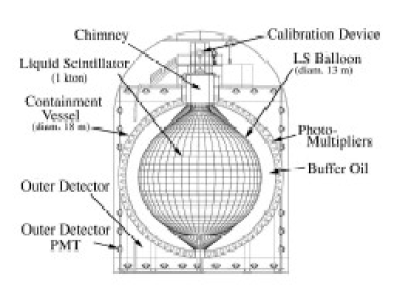
Figure 19: Schematic view of the KamLAND detector

The experiment target consists of 1 kton of ultra pure liquid scintillator [20% pseudocumene, 80% mineral oil (dodecane), and 1.52 g/l PPO] contained in a 13–m–diameter transparent balloon. The target is viewed by 1,879 PMTs, of which 1,325 are 17–inch and the balance 20–inch, providing a photocathode coverage of about 34%. The PMTs are bolted to a 18–m–diameter stainless steel sphere (containment vessel). The volume between the balloon and stainless steel sphere is filled with mineral oil, buffering the target against natural radioactivity in the PMTs, stainless steel sphere, and surrounding rock and against fast neutrons generated by muon spallation outside the containment vessel. A UV–transparent acrylic sheet 3 mm thick mounted just in front of the PMT faces acts as a barrier to radon emanating from the PMTs. The stainless steel sphere is enclosed by the outer detector, a water Cerenkov muon detector which consists of a cylindrical tank of pure water viewed by 225 PMTs. The detector is located in the Kamioka Underground Observatory, in the cavern formerly occupied by the Kamiokande Experiment. The rock overburden exceeds 2,700 mwe, resulting in a muon rate through the experiment target of about 0.34 Hz.

There are 16 commercial nuclear power plants in Japan, accounting for 97% of the neutrino flux at KamLAND. The bulk of the flux–about 80%–is due to reactors 138–214 km away. The mean $\bar{\nu}_{e}$ energy, weighted by the inverse beta decay cross section, is about 5 MeV. Records on thermal power, burn–up, and fuel–exchange are furnished to the experiment on a continuing basis by the plant operators. The total reactor power varies by 20–30% throughout the year (down to 50% in 2003), which provides a means of subtracting backgrounds by investigating the correlation of the event rate with reactor power.

The primary trigger for the experiment presently requires 200 PMT hits, corresponding to an energy threshold of about 0.7 MeV. Following each primary trigger, the threshold is lowered to 120 PMT hits for 1 ms to detect low–energy delayed activity. In addition to being discriminated for the trigger, the PMT voltages are sampled and digitized by waveform analyzers (ATWDs). There are two ATWDs per PMT, allowing two–step sequential events to be fully recorded. The ATWD sampling rate is about 630 MHz, and 128 samples are acquired per waveform. Signals in the outer detector are recorded as part of the standard data stream for offline analysis. The trigger rate is about 20 Hz. The amount of data recorded per day is about 150 GB.

Energy estimation, vertex reconstruction, and detection efficiency are calibrated using gamma sources ranging in energy from 0.279 MeV to 7.7 MeV, neutron sources (Am–Be), and light flashers (LEDs and lasers). Sources are deployed along the vertical axis of the experiment by winch operated from a sealed glove box at the top of the detector; in addition, there are blue LEDs permanently mounted on the stainless steel sphere. Besides detailed calibrations carried out from time to time, the detector is monitored on a weekly basis with gamma sources. Natural sources, namely spallation neutrons, cosmogenics, and natural radioactivity, are also used for detector calibration.

The signal process is inverse beta decay

$$\bar{\nu}_{e}+p\rightarrow e^{+}+n.$$

The experimental signature is a prompt energy deposit of 1–8 MeV, due to the positron kinetic energy and annihilation, followed an average of 200 $\mu$s later by emission of a 2.2 MeV gamma from neutron capture on hydrogen. Exploiting the delayed coincidence is key to controlling backgrounds.

Following the first publication [7], we now describe event selection, background estimation, experimental uncertainties, and interpretation of data in the context of $\bar{\nu}_{e}$ disappearance and neutrino oscillations.

The cuts applied to select inverse beta decay candidates are the following:

1. Both the prompt and delayed subevent vertices lie within 5 m of the detector center.

2. The delayed subevent occurs within 0.5–660 $\mu$s after prompt subevent.

3. The prompt and delayed subevent vertices are separated by less than 1.6 m.

4. The delayed subevent energy lies between 1.8 and 2.6 MeV.

5. The delayed subevent vertex lies more than 1.2 m from the central vertical axis.

6. The event occurs at least 2 s after a showering muon (energy deposit greater than $\sim$3 GeV) and at least 2 s after, or more than 3 m away from, any other muon track.

7. The prompt subevent energy is greater than 2.6 MeV.

Cut 1 is applied to control backgrounds due to natural radioactivity in the balloon system, the PMTs, and beyond and backgrounds due to muon spallation in the surrounding rock. Cut 5 controls backgrounds from natural radioactivity in the thermometers suspended in the central detector. Cut 6 is made to suppress backgrounds from cosmogenics, e.g. ⁸He and ⁹Li, and spallation due to muons passing through the central detector. We have included Cut 7 to eliminate the low–energy region in which terrestrial radioactivity is expected to contribute.

The efficiency of the Cuts 2–5 plus Cut 1 applied to the delayed subevent on inverse beta decay events is 78.3$\pm$1.6%. The effect of Cut 6 is taken into account in the livetime calculation.

Applied to the data set acquired March 4 – October 6, 2002, which includes in all 145.1 d of live time, 54 events are selected. Figure 20 shows the energies of the delayed versus prompt subevents after all cuts have been applied but Cuts 4 and 7.

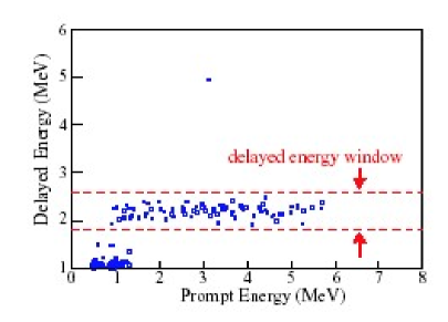
Figure 20: The energies of the delayed subevents in KamLAND versus the energies of the respective prompt subevents for events passing all selection cuts but Cuts 4 and 7 (see text).

The contribution to the event sample from accidental delayed coincidences has been estimated by repeating the event selection with an off–time delayed coincidence window. The contribution is found to be small, namely 0.0086 $\pm$ 0.0005 events.

The residual cosmogenic background in the candidate sample has been estimated by analyzing the time and spatial correlations between muon tracks and event candidates. The result of this analysis is that the expected cosmogenic contribution to the sample is 0.94 $\pm$ 0.85 events.

Fast neutrons from muon spallation can easily mimic inverse beta decay events and thus are a potentially dangerous background. Their contribution is, however, suppressed by the fiducial volume cut (r $<$ 5 m). The contribution of this background has been estimated from a sample of muon events–where the muon misses the inner detector–which contain an inner detector event that passes the event selection cuts. The vertex distribution for this sample is extrapolated into the fiducial volume and then normalized to the muon track reconstruction inefficiency. This approach yields the result that less than 0.5 events are due to fast neutrons.

In summary, the total expected background in the event sample is 0.95$\pm$0.99 events.

For comparing the observed events with the expected number of events under different scenarios (no oscillations, two–flavor neutrino oscillations, etc.), a number of quantities enter which carry systematic uncertainties. These quantities and the estimated magnitudes of the systematic uncertainties are: total liquid scintillator mass–2.1%; fraction of mass within fiducial volume–4.1%; energy scale at 2.6 MeV–2.1%; selection cut efficiency–2.1%; experiment live time–0.07%; reactor power–2.0%; fuel composition–1.0%; finite lifetime of fission products–0.3%; neutrino spectra–2.5%; and inverse beta decay cross section–0.2%.

Adding the individual contributions in quadrature, the total systematic uncertainty is estimated to be 6.4%.

The integrated number of events expected for no disappearance is 86.8 $\pm$ 5.6 events. Figure 21 shows, including accidental background and $\bar{\nu}_{e}$’s from terrestrial radioactivity, both (a) the expected prompt energy distribution for the case of no disappearance and (b) the corresponding distribution for the observed events.

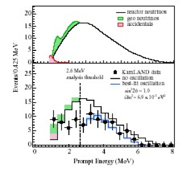
Figure 21: Upper panel: Prompt KamLAND energy distributions for the expected (no disappearance) case. Lower panel: same as upper panel except binned in energy and including energy spectrum of observed events. Also shown is the result of a fit to the observed events above 2.6 MeV in terms of two–flavor neutrino oscillations; the shaded area superimposed on this fit indicates the systematic uncertainty in the best–fit result.

Accounting for the $\sim$1 background event, the 54 events observed above 2.6 MeV are inconsistent with the hypothesis of no disappearance at the 99.95% confidence level.

One may instead interpret the observed events in terms of two–flavor neutrino oscillations. Figure 22 shows the result for analysis of the total rate and of the rate and shape of the energy spectrum. The best fit to the rate and shape gives $\Delta m^{2}$ = 6.9$\times$10^-5 eV² and $\sin^{2}2\theta$ = 1.0. Assuming CPT invariance, it can be seen that the KamLAND observation is consistent with the MSW LMA solution to the solar neutrino problem and further restricts the allowed LMA region.

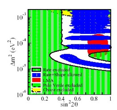
Figure 22: Excluded regions of neutrino oscillation parameters for the rate analysis and allowed regions for the combined rate and shape analysis from KamLAND at 95% CL At the top are the 95% CL excluded region from CHOOZ and Palo Verde experiments, respectively. The 95% CL allowed region of the LMA solution of solar neutrino experiments is also shown. The solid circle shows the best fit to the KamLAND data in the physical region

In summary, since starting to take data in January 2002, KamLAND has observed reactor anti–neutrino disappearance with a very high level of confidence (99.95%). The MSW LMA solution is the only neutrino oscillation solution to the solar neutrino problem which is consistent with the KamLAND result and CPT invariance.

KamLAND continues to take data and make improvements to the detector and data analysis. These improvements include inclusion of the 20–inch tubes in the data analysis, installation of a 4$\pi$ deployment system for calibration sources, deployment of a $\beta$ source and additional gamma sources for better understanding of the detector energy response, and development of a full detector simulation. These improvements are expected to reduce significantly the uncertainties on the amount of mass contained within the fiducial volume, the energy scale at 2.6 MeV, and the selection cut efficiency. Improvement in the accuracy to which the reactor–related quantities, e.g. reactor power, are known is also anticipated. Achieving a total systematic error in the range of 3–4% appears realistic, in which case the dominant source of error for the experiment after several years of data taking will be statistical.

5 Detector Design

From the discovery of the neutrinos by Reines and Cowan [81] at Savannah River to the evidence for $\bar{\nu}_{e}$ disappearance at KamLAND [7], reactor neutrino experiments have used the same fundamental design. A single detector, placed at a given baseline distance from the reactor core, is used to measure the absolute flux and energy spectrum of $\bar{\nu}_{e}$ through the inverse beta decay process. As detectors have moved further away from the reactors over the years, it has become more important to shield them from background sources (primarily derived from cosmic muons) since the flux of reactor neutrinos falls with the square of the baseline distance. Experiments at baseline distances of one kilometer or more (Chooz, Palo Verde and KamLAND) have accomplished this by placing their detectors at significant depths underground.

5.1 Detector Target and Buffer

Any detector to measure reactor antineutrinos takes advantage of the inverse beta decay reaction:

$$\bar{\nu}_{e}p\rightarrow e^{+}n$$ (17)

followed by neutron capture and measures a coincidence between the signal from the $e^{+}$ and the neutron. The prompt positron will exhibit 1-8 MeV of visible energy when it annihilates, with a minimum energy from the $e^{+}e^{-}$ masses. The inverse beta decay reaction takes place on hydrogen, an element which occurs in water and all forms of liquid scintillator. Liquid scintillator has been used in CHOOZ, KamLAND and earlier experiments. Since scintillator consists of long organic molecules, one issue is to accurately determine the hydrogen fraction.

A neutron will capture on hydrogen and form deuterium giving gamma rays with an energy 2.2 MeV. This is the process measured in the large KamLAND experiment. Smaller experiments find it advantageous to load the scintillator with about 0.1% Gadolinium (Gd) which has a very large capture cross section for neutrons and also leads to a higher energy gamma shower, 8 MeV. In CHOOZ, 86.6 $\pm$ 1.0 % of the neutrons were captured in Gadolinium [10]. However the Gadolinium lowers the optical attenuation length and, more importantly, time dependent effects have been noticed regarding the optical properties. Time dependent effects will need to be minimized or thoroughly understood, at least in the way that they might manifest themselves differently in multiple detectors. Gd loaded targets are presently favored for a new reactor experiment, but if the time dependent effects cannot be adequately controlled, then a larger detector for a future 8000 t GW y experiment might consider not using it.

There are some issues to be considered in the choice of scintillator. In some forms, Gadolinium loaded scintillator is not compatible with an acrylic vessel. One example is pure PXE with 0.1-0.15% Gd. The compound Gd-ACAC or Gd-Carbolylate is being investigated at Max-Plank-Institut für Kernphysik in Heidelberg. The aromatic component is $C_{16}H_{18}$ which has a low concentration of hydrogen. The alternative is 40% PXE/PC with 60% mineral oil and 0.1% Gd, the cocktail already used by Palo Verde. It is compatible with acrylic, though there have been problems of degradation of attenuation length versus time seen in certain solutions of as much as 2 cm/day. Aromatics and alkenes provide more hydrogen per unit volume than pure PXE. To compare, 10 cubic meters of PXE weigh about 10 tons and contain $5.15~{}\times 10^{29}$ atoms of H, compared with 10 cubic meters in CHOOZ, which weighed 8.54 tons and contained $6.87~{}\times~{}10^{29}$, an increase of 33%.

The glass in the phototubes themselves emits gamma rays from which the fiducial volume must be shielded. This will be accomplished with a scintillating buffer, a non-scintillating buffer, or both.

The advantage of a scintillating buffer is that the positron energy is fully contained. No neutron will capture on the Gd in the buffer (because there isn’t any), but a positron which crosses the target/buffer boundary will not lose any less visible energy if the buffer is scintillating, so the minimum energy of 1 MeV is seen, i.e. $E_{threshold}<E_{min}(e^{+})$. This reduces a systematic error which was 0.8% in CHOOZ to 0% [82].

The disadvantage of a scintillating buffer is that it contributes to a greater accidental background from ⁴⁰K radioactivity present in the PMTs. This would argue for the presence of both scintillating and non-scintillating buffers. One conceptual design of a detector with two buffers is shown in Figure 23.

The inner volume of the conceptual 10 ton detector design shown in Figure 23 is 1.4 m (radius) Gadolinium loaded scintillator to serve as the neutrino target. The size of this volume is determined by the desired target mass, but may be constrained by the overall size of the target hall. This volume will serve to well define the fiducial volume in which neutron capture takes place. The 2nd volume is 0.35 m scintillator without Gadolinium, the gamma catcher. This distance is defined by the absorption length of gamma rays and assures that all gammas from neutron capture in the fiducial volume are visible. With a scintillating buffer, there is no need for a fiducial volume cut. The 3rd volume is 1.0 m mineral oil without scintillator, the PMT buffer. This boundary, a few photon interaction lengths, buffers the central region against photons coming from radioactivity associated with the phototubes. The outside volume from 0.6 to 1.0 m thick is filled with water has an independent set of phototubes is used to veto cosmic ray muons and other entering tracks. Alternatively, there may be layers of active and passive material to serve as a cosmic veto. There may also be an additional meter of water in some directions to serve as a neutron catcher.

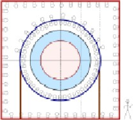
Figure 23: Conceptual detector design. Inner volume is Gadolinium loaded scintillator. The second volume is non-doped scintillator. The third volume is mineral oil. Outside is veto region.

The disadvantage of the second buffer is that it makes a detector larger for a fixed fiducial volume. The size of the detector will affect the civil construction costs of the detector hall and tunnel, which are expected to be the dominant costs for the experiment. This is especially true if movable detectors are considered, because the path on which the detector moves will need to be that much larger. Therefore the advantage of the buffer will have to be evaluated quantitatively together with the construction costs for any site. For example, in a design with two buffers, 2.7 m of diameter is needed for the buffers. This means that there is a maximum of 15 ton target volume if the detector needs to be moved through a tunnel with a diameter of 6 meters.

5.2 Mechanical Structure

The structure will be a significant part of the mechanical design of the detector. There will need to be an optical structure, to separate the target from any buffer regions and another one to separate the buffers from each other. The optical structures will perhaps be made from acrylic. KamLAND and Borexino have had success using nylon balloons, but a flexible container is probably not a good way to maintain fiducial volumes to better than the 1% accuracy required for this experiment. There will also need to be an opaque structure to separate the buffers from the veto region and to support a frame which holds the PMTs. This will perhaps be made from steel. The acrylic vessels will need to have access ports through which the volumes can be filled and also in which sources can be put in and moved around. All structures will need to be designed so that proper buoyancy can be maintained during fill.

5.3 Muon veto

A sufficient volume of water is needed to shield the detector from neutrons created by muon cascades outside the veto region. The veto region will need to have enough phototubes to efficiently tag all muons which enter the muon region. If movable detectors are chosen, it is not foreseen that the veto detector would be movable. But it would then need to be designed so that the fiducial target could be removed.

Another design for a muon veto involves layers of passive shielding, such as concrete, and a layer or layers of high efficiency planar detectors to measure the incoming muon.

There are reasons to also consider passive shielding outside the veto region, depending on the conditions of local radioactivity and the orientation of any shafts or tunnels.

5.4 Liquid Handling System

There will need to be a safe and careful system for handling and testing the different liquids. There will need to be very accurate measurements of the volume of each liquid during fill, particularly in the target region. Spills of liquid scintillator will need to be avoided, particularly with regards to any contamination of ground water.

The conceptual design for the detector shown in Figure 23 is accompanied with the need to handle four different liquids: Gd loaded scintillator, scintillator, mineral oil, and water. All will need to be maintained with well-known optical properties. One possible solution for the issue of optical changes in Gd loaded scintillator is mixing through recirculation, with or without filtering. A recirculation system will have to be designed to evenly affect each liquid throughout its volume. Filtering might be designed to deal with optical degradation due to organic compound production, but it may also remove Gd, and a system which removes and precisely reloads solutions in the liquid may be difficult to accomplish. Another concern about recirculation is the introduction of microbubbles, which could both change the optical properties as a function of time and also lead to small time-dependent density changes. The advantages and disadvantages of recirculating each volume will need to be carefully reviewed, probably by extensive testing.

5.5 Detector Shape

The ideal detector has a spherical design. This design offers the lowest ratio of surface to volume, which implies the least number of photomultipliers per ton, the lowest surface radioactivity, the most buffer material to absorb external neutrons, the lowest cross section to cosmic rays, and hence the lowest total mass per ton of target. With SNO, KamLAND, MiniBooNE and Borexino, there is a great deal of experience with the design and construction of spherical liquid scintillator detectors. They also have the simplest parameterization of optical effects, which will be even more important due to the low attenuation length of Gd loaded scintillator.

Nevertheless, if movable detectors are chosen, cylindrical detectors offer some advantages. The target mass must be moved in an area less than 6 meters squared (the maximum size of most economic tunnels). To achieve a 50 ton or greater mass, the detector must be cylindrical. As a comparison, in Figure 24 there is a 50 ton cylindrical target and a 25 ton spherical one. Both detectors have a 70 cm pure oil buffer, and 20 cm region to shield the PMTs, together with 20% PMT coverage. Assuming that only one near detector is needed in each case, then for a 50 ton active volume for the far detector, 2372 PMTs are needed for 2 cylindrical detectors compared to 2382 for 3 spherical ones. For 75 tons, the result is 3156 for 2 cylindrical detectors and 3176 for 4 spherical ones. The costs of the vessels cannot be ignored, but in the limit where the detectors costs are dominated by PMT and channel counts, this would argue toward multiple spherical detectors over larger cylindrical ones.

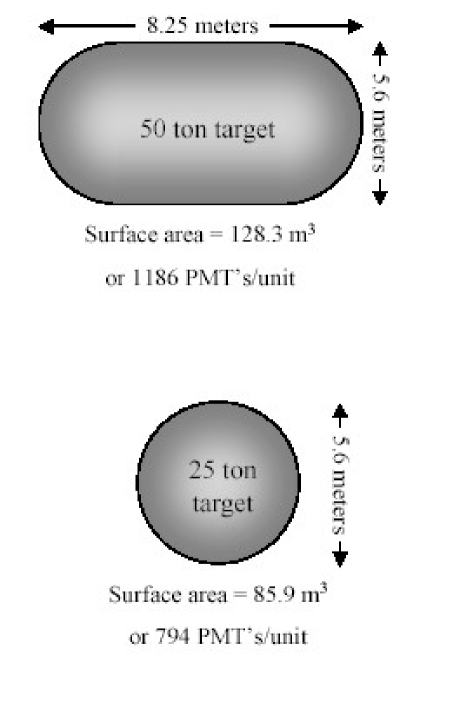
Figure 24: A comparison of spherical and cylindrical detectors

5.6 Movable Detectors

The purpose of designing movable detectors is to be able to move the identical far detector to the near detector location for part of the running period and have a head-to-head calibration of the relative number of events. Assuming that there is no additional error introduced by the act of moving the detectors, the uncertainty of this efficiency ($\varepsilon$) is

$$\sigma_{\varepsilon}=\varepsilon\sqrt{\frac{2}{N}}$$ (18)

where N is the number of events measured during the calibration.

Designing the detectors to be movable will certainly have a great effect on the detector design. However, it will have an even larger effect on the tunneling requirements. Let’s consider the options for an experiment with two detectors and a flat overburden. Three scenarios are shown in Figures 25, 26, 27. In Scenario One, there are two shafts and a tunnel connecting them in which the detector can be moved. The shaft for the near detector may be placed away from existing infrastructure such as substations and parking lots, outside the security fence. This is probably the easiest solution for detector design, but the most expensive for civil construction. The second solution takes advantage of sloped access and the fact that the near detector does not need to be as deep as the far detector. The angle of approach for the access ramp could be from any convenient direction. In scenario three there would be two shafts and a surface detector transport procedure. The detector would be raised to the surface by a crane or elevator system and transported on surface rails. This may be the cheapest option, but it may also be a more complex and risky procedure.

Figure 25: A scenario with two shafts and a connecting tunnel

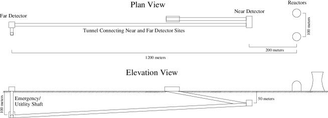
Figure 26: A scenario with sloped access

Figure 27: A scenario with two shafts

5.7 Multiple Detectors

Assuming that backgrounds and deadtime issues are under control, the statistical power of the experiment is driven by the size of the far detector. The near detector will have a larger event rate by a factor of $(L_{2}/L_{1})^{2}$, so for the same statistical power, it might be reasonable to make the near detector smaller. Any difference in size between the two detectors, however, compromises the ability to cancel systematic errors, and this experiment’s goal is to measure the neutrino flux with a much better systematic error than has previously been achieved. This dilemma has led to consideration of several other detector configurations:
Multiple Far Detectors It might be desirable, for example, to make a 20 ton near detector, and multiple identical 20 ton far detectors, perhaps five. This would be a way to get more fiducial mass at the far detector, and also a possible way to stage some of the experiment. The multiple far detectors would be a smaller fiducial mass than a single larger detector with the same channel count. However, they would provide additional checks on some of the systematic errors of multiple detectors.
Multiple Locations Another variation of this idea is shown in Figure 28 where multiple identical detectors are used. In this example, a small 5 kiloton detector is placed near the reactor, and another one a few hundred meters away, along with a larger 30 ton detector, which is repeated at 1.7 km. Again, there are multiple opportunities to study possible systematic errors and staging possibilities. This scheme provides additional opportunities for cross calibration of each detector.

One possible attraction of the multiple location idea is that the optimization of distance for the 400 t GW y experiment could be at a different location than for the more sensitive 8000 t GW y experiment. This is because the optimum location, discussed in Section 3 is different for the rate test and the energy shape test. The rate test is more powerful for the lower statistics and the shape test for the higher statistics experiment. Unfortunately, the optima discussed in Section 3 does not seem to lend itself to a solution that involves staging detectors in a natural way.

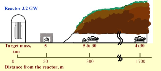
Figure 28: Possible layout for multiple detectors.

6 Calibration

6.1 Introduction

Calibration provides the information required to: (a) reconstruct the energies and positions of the prompt and delayed sub-events, (b) tune the experiment’s simulation software to match as closely as possible the data without introducing biases and so compute the detection probability as accurately as possible, and (c) reliably estimate the magnitude of uncertainties in detector response. Although it will not be further discussed in what follows, calibration should also enhance the capability to discriminate between signal and background processes, e.g., through accurate characterization of detector response to neutrons with energies typical of spallation products and through development of a trigger to record muon-produced neutron capture in the experiment.

What calibration accuracy is required? Based on the record of previous experiments similar in design to those being considered for a next generation reactor neutrino experiment, the contribution from calibration to the overall uncertainty for a single detector can be limited to a few percent. The calibration program outlined should aim toward controlling the single detector uncertainty at this level. To achieve an overall systematic uncertainty on the relative far-to-near detector event rate at the percent level, it is further required that the calibration of the near and far detectors–as well as detector design, operation, and data analysis–be as identical as possible.

6.2 Calibration System Design Considerations

A calibration program capable of achieving the accuracy specified above will have the following characteristics:

• Calibration sources that are precisely deployable throughout the entire active target region of each detector. At representative locations in each detector, it should be possible for some calibration sources to pass through and beyond the outer boundary of the active target. The requirement that sources be deployable throughout the entire target region and somewhat beyond its boundary at representative locations can be relaxed if events in the boundary region are excluded from analysis. Whatever region is used for analysis, it should be considered important that calibration sources can be placed at any point in this region. The uncertainty in the position of the calibration source should be about 5 cm or less, assuming the lineal dimensions of the detectors are on the level of several meters; and the deployment system and calibration sources should be designed to minimize shadowing and absorption.  These requirements require novel mechanical designs for source insertion and removal that may be quite challenging.  Indeed, considerable R&D may be required to establish that calibration methods successfully demonstrated on the $\sim$12 ton CHOOZ detector can be scaled up to 50+ ton devices being contemplated.

• Multiple calibration sources that include the following:

  1. Point gamma sources spanning the energy range from inverse beta decay threshold to the highest achievable energy for calibrating energy estimation, vertex finding, and detection efficiency. Readily available radio–isotopes that would be suitable include Cs–137 (0.662 MeV), Ge–68 (2 $\times$ 0.511 = 1.022 MeV), Zn–65 (1.116 MeV), and Co–60 (1.333 + 1.173 = 2.506 = MeV). Sources with energies in the range of 5–8 MeV would also be desirable, but are typically difficult to fabricate and deploy due to short half lives and low branching ratios for the gammas of interest. A development effort to design and deploy gamma sources in this energy range may well be worthwhile. At least one of the gamma sources should have its visible activity known to $\sim$1% for the purpose of measuring detection efficiency, and a range of gamma energies is needed in order to help measure the effects of quenching and Cerenkov radiation on light output. The Ge–68 source is particularly attractive because it probes the detector response at inverse beta decay threshold.

  2. $\beta$ source. Using gammas alone, it may prove difficult to determine the absolute energy scale for positrons to better than 1%. Some studies of future reactor neutrino experiments have assumed that the absolute energy scale is known to 0.5%. To achieve this level of precision, use of a $\beta$ source, preferably a $\beta^{+}$ source, should be planned. Controlling uncertainties in the $\beta$ energy spectrum from capsule shadowing and absorption in the encapsulation materials will be a challenge, however.  A deployment of a Ge-68 source in solution with the liquid scintillator has been suggested [88] to solve to this problem and it would also provide a truly homogeneous and in situ calibration for gamma rays.

  3. Tagged neutron source for measurement of the neutron detection efficiency. Am–Be is a good candidate for such a source. The 4.4 MeV gamma can be used to tag single neutron emission. Corrections for the differences between the Am-Be neutron energy spectrum and the inverse beta decay neutron energy spectrum would be made using simulation. Important also is that such a source provides additional gamma calibration points: (i) 2.225 MeV from capture of neutrons on protons and (ii) 4.443 MeV provided that a significant fraction of the neutrons can be moderated before they enter the scintillator. Moderated Am–Be sources have been used successfully for energy calibration in other experiments.  The CHOOZ experiment also made good use of Cf neutron sources.  These produce a continuous neutron and gamma spectrum but offer the advantages of higher rate for studies of homogeneity.

  4. Variable intensity light flasher. Possible sources include UV lasers and UV LEDs. As practically point-like sources of fast pulses of controllable amplitude, such sources are valuable for calibrating vertex reconstruction (which is usually based on PMT timing with charge-dependent corrections), measuring PMT gain and interpolating the detector response between gamma calibration points.

• Integration of the calibration system as an integral part of the data acquisition, event reconstruction, and detector simulation software:  A large fraction of events read out over the course of the experiment will be various calibration triggers.  The acquisition of this data must not adversely affect dead time for the experiment.  Careful design of triggering and run control is essential, and processing of calibration data must take place quickly to help identify shifts in detector performance.

• Simulations. Because it is not possible to deploy a source that mimics inverse beta decay in the reactor neutrino energy range, detector simulation ultimately plays an important role in estimating the detector response to this process. As such it requires an accurate and detailed description of the detector (regarding materials, geometry, and optics) and of the calibration sources and the devices used to deploy them. Generation and transport of photons to the PMT photocathodes must be modeled accurately, as should also be the digitization of PMT pulses and effects of discriminator thresholds. Simulated data must be reconstructed with the same software as real data. The event generators for inverse beta decay and the calibration processes must be accurate and detailed.

• Construction of identical calibration programs for the near and far detectors in both hardware and software. So far as is possible, the calibration sources should be the same, or at least fabricated by identical means; and the deployment systems should likewise be identical in design. If the near and far detectors have different sizes, designing the deployment systems to be the same to within overall scale should be a consideration.  The scope and magnitude of the calibration programs should be planned so that any calibration carried out for one detector can also be carried out for the other at nearly the same time.

6.3 Concluding Remarks

What is ultimately required for adequate calibration will not be fully known until experience has been gained on the detectors running under normal conditions. However, given past experience and the experimental design and goals, it is clear that the baseline calibration program should have the capability of precisely deploying well–understood calibration sources at any desired position throughout–and preferably beyond, in the case of gamma and neutron sources–the active volume of the detector. Control of systematics will be aided by the ability to deploy the same sources in both the near and far detectors. The calibration program effort should be matched by an effort to develop a full detector simulation tuned and checked against the calibration data; this simulation program can then be used to extend understanding of the detector into areas for which calibration data is not available.

7 Detector Overburden and Backgrounds

Backgrounds will be an important consideration in site selection and detector design. They can be classified into two distinct sources: (1) internal backgrounds associated with radioactivity in the materials of the detector and lab site, and (2) external activity associated with cosmic rays and their interaction daughters. The former is a well-understood technology that has been solved many times over several decades by a combination of materials selection, self-shielding, and signal enhancement via addition of neutron absorbers that boost the energy of the neutron capture reaction. It is not expected that this will be a major problem.

Cosmic ray activity is typically more serious and in most cases requires an underground location of at least at least a few tens of meters of water equivalent (m.w.e.) for even rather small detectors of less than 1 ton. The limiting factor is typically the flux of neutrons associated with muon nuclear interactions in the detector and in the surrounding rock. Table 5 is a brief summary of some previous reactor experiments done over the last 25 years. As can be clearly seen, longer distances have necessitated larger detectors, which have in turn required underground sites to reduce the cosmic ray muon flux and hence the flux of external neutrons.

Table 5: Summary of some previous reactor experiments

Name	powerth	mass	distance	depth	comments
	(GW)	(tons)	(m)	(mwe)
ILL [89]	0.057	0.32	8.76	7	${}^{3}He$ + scint. PSD
Gosgen [90]	2.8	0.32	38/46/65	9	same as ILL
Rovno [91]	1.4	0.43	18		Gd scint.
Krasnoyarsk [92]	1.6	0.46	57/231	600	${}^{3}He$ only
Bugey 3 [93, 94]	2.8	1.67	15/40/95	23/15/23	${}^{6}Li$ + scint. PSD
Savannah R. [95]	2.2	0.25	18.2/23.8	$\sim 10$	Gd + scint. PSD
CHOOZ [10]	4.4	5	1000	300	Gd + scint.
Palo Verde [75]	11.6	11.3	800	32	Gd + scint.
KamLAND [7]	$\sim 80$	408	$\sim 180,000$	2,700	scint.

The final design of this experiment will be a trade-off between several conflicting goals: (1) the desire to have the near and far detectors be as identical as possible to allow cancellation of systematic errors due to detector geometry, (2) the desire to have the near detector be small to avoid muon-related backgrounds and expensive overburden requirements, and (3) the desire for a far detector of size large enough to give an acceptable event rate. Backgrounds will be a major consideration in the final design and so we have developed some general constraints based on the measurements of previous experiments.

7.1 Types of Backgrounds

The double coincidence afforded by $\overline{\nu}_{e}+p\rightarrow n+e^{+}$ followed by $n+p\rightarrow d+\gamma$ requires that two events appear within a given time and space window, typically 25-200 $\mu$s and $\leq 1$ m. The space requirement is usually enforced either by vertex fitting or detector segmentation. Events that are inherently “singles” are therefore strongly suppressed as they must appear by accidental coincidence in the correct window. Examples are internal radioactive decay, stopping cosmic ray muons, and external gamma events.

Correlated backgrounds are more serious. Such events can mimic the reactor anti-neutrino signal and there can be significant uncertainties associated with the rate. The majority of correlated backgrounds come from events associated with cosmic ray activity. Examples are fast neutrons from muon nuclear interactions, muon capture reactions from stopped muons, and excited nuclei from muon spallation reactions that may de-excite by neutron emission.

In many cases experiments have been placed deep enough underground to sufficiently suppress the cosmic ray muon flux (e.g. KamLAND). In other cases a segmented detector was used to allow more precise cuts on vertex location and partial detector vetoing (e.g. Palo Verde and Bugey). In cases where the detector is small and close to the core, only minimal shielding was required (e.g. Savannah River). Table 6 shows the effective detection rate for some previous experiments. This is the daily rate of neutrinos detected (corrected to a distance of 100 m) while the detector is operating per ton of fiducial target per GW of reactor power . Variations of a factor of two are seen, mostly due to the overall efficiency constraints imposed by the necessity to reject backgrounds. Detectors which are segmented and near the surface (ILL, Gosgen, Bugey, Palo Verde) tend to have less efficiency than monolithic ones (Savannah River, CHOOZ, Rovno, Krasnoyarsk, KamLAND) with sufficient shielding relative to the detector size.

Name	effective rate at 100 m
	($d^{-1}t^{-1}GW^{-1}$)
ILL	15.7
Gosgen	14.4/14.5/13.6
Rovno	46
Krasnoyarsk	35/41
Bugey 3	22/19/19
Savannah River	50/54
CHOOZ	51
Palo Verde	12
KamLAND*	61

Table 6: Effective $\overline{\nu}_{e}$ detection rate. (*) The KamLAND rate is based on the expected rate of 86.8 events in 141 days.

In the discussions below we use the experience of previous reactor experiments and estimate depth and shielding requirements for both a “near” ($100$ m) and a “far” ($1.5$ km) detector. It is assumed that the basic detector module is roughly 10 tons, with the far site requiring several such modules and the near site one.

7.1.1 Accidental Coincidences

Single, uncorrelated events may result from radioactive decay from internal materials such as steel and glass, external gammas from the shielding or surrounding laboratory, or from cosmic ray muons if the depth is shallow. The coincidence rate $R$ for two uncorrelated events with rates $R_{1}$ and $R_{2}$ to occur in a time window $w$ is given by :

$$R=R_{1}R_{2}w$$ (19)

This rate must be compared with expected neutrino interaction rates for a typical 10-ton scintillator detector. For the near (far) module this would typically be about 1000 (4.5) events/day/GW with 100% efficiency. A typical reactor is assumed to be 3 GW thermal, giving a signal rate of 3000 (13.5) events/day. Using equation 19 and setting a criterion that the accidental rate should be less than 1% of the actual event rate, restrictions on various sources of “singles” can be estimated.

Cosmic Ray Muons: Cosmic ray muons can produce accidental coincidences in several ways: (1) straight-through muons mimicking positrons or neutron capture (unlikely), (2) decay of stopped muons giving an $e^{\pm}$ followed by an accidental coincidence of a muon capture that gives a neutron, and (3) a stopped muon decaying to an $e^{\pm}$ followed by the accidental coincidence of a neutron from spallation. In (2) and (3), the rate must be less than the rate of accidentals from (1) since they are initiated by somewhat rare reactions from (1). Correlated background from these types of events is treated in a later section.

Taking $R_{1}=R_{2}=R_{\mu}$, where $R_{\mu}$ is the muon rate through the detector, and a typical neutron capture time of $25\mu$s which would imply a window of roughly 100 $\mu$s for 98% efficiency, then allowed muon rate through the detector is 1.9 Hz (0.12 Hz) for the near (far) detector. This is to be adjusted for muons that can be tagged. Most all previous experiments had muon vetoes (see Table 7) that were better than 95% efficient in tagging muons. Therefore the acceptable muon rates can be conservatively adjusted up by at least a factor of 20. This would correspond to a depth of about 85 m.w.e. (350 m.w.e. for far) for a 10 ton module. Figure 29 shows the percentage of the signal this background would be as a function of depth.

Figure 29: The rate of muon accidental coincidences as a fraction of the expected signal as a function of depth. Left (right) is for the near (far) detector.

This estimate is conservative in that it does not take into account the low probability that a muon is misidentified as a positron and/or capture gamma. In addition, vertex cuts may further reduce the possibility of a chance coincidence. What can be said is that at these depths single muon accidentals will not be a problem as long as the neutron capture time is kept short by the addition of gadolinium or other absorber.

Table 7: cosmic ray rejection

Name	muon rate	veto efficiency	dead time
	($s^{-1}$)	(%)	(%)
ILL	250	99.8	8
Gosgen	260/300/340	99.8	8
Rovno	350	99	7
Bugey 3		99.5	2
CHOOZ	1		2
Palo Verde	2000	96	2
KamLAND	0.3	92	11

Internal Radioactivity: Backgrounds from internal radioactivity come from many sources: (1) $U/Th$ in detector materials (such as scintillator), (2) $U/Th$ and ${}^{40}K$ activity from PMT glass, and (3) $U/Th$ in stainless steel, to mention a few. Radon incursions may also take place from penetration through piping flanges, calibration device insertion, or any place where detector scintillator contacts the radon-laden air common in underground sites.

The singles rate from these sorts of backgrounds is a strong function of the detector threshold. This is because most long-lived beta activity is below 2 MeV and energetic alphas are strongly quenched, typically with factors of 0.1 or less such that they have visible energies of less than 1 MeV. The effect of these events on the coincidence rate is therefore a strong function of threshold. Table 8 shows the threshold for recent reactor experiments. 1 MeV is clearly achievable if sufficient care is taken in materials selection, radon exclusion, and the allowance of sufficient shielding from PMTs via a non-scintillating buffer region and self-shielded fiducial volume. As an example, assuming a ${}^{238}U$ level of $10^{-14}$ $g/g$ in the scintillator (about 100 times less stringent than the levels required by Borexino) and only taking into account the 3 beta decays with $Q>1$ $MeV$ results in a singles rate above 1 MeV of about 0.004 Hz in a 10 ton detector. This is conservative in that it assumes all the betas are above threshold. This level is consistent with a more detailed study done for the KamLAND detector in the U.S. proposal. In this study similar rates are obtained for ${}^{232}Th$ and ${}^{40}K$ at levels that can be achieved by reasonably careful control of detector materials and possibly scintillator washing and/or filtration. Care is also taken to move the PMTs well back from the fiducial volume.

Radon-laden air in enclosed spaces can sometimes reach as high as 1200 $Bq/m^{3}$ [96]. Since the ${}^{222}Rn$ chain includes ${}^{214}Bi$(Q=3.272 MeV) allowing such levels inside the scintillator would result in unacceptable background levels. In addition, ambient radon levels are often seasonal and/or dependent on local weather conditions. It is therefore necessary to control radon levels in the laboratory areas and to take precautions to ensure radon cannot diffuse into the scintillator via use of radon-free nitrogen blankets, radon impermeable o-rings and gaskets in all piping, and the use of detector materials low in radon emissivity. For example, the radon level in the Super-Kamiokande water is reduced to around $3\times 10^{-3}$ $Bq/m^{3}$ by taking such precautions. Similar low levels in a 10-ton detector would result in a coincidence rate of around 0.003 $d^{-1}$, which is completely negligible.

Table 8: $e^{+}$ energy measurement performance of past reactor experiments.

Name	threshold	precision	resolution	variation
	(MeV)	(%)	(% FWHM)	(%)
ILL	0.9	2	18	5
Gosgen	0.7	2	18	5
Rovno	0.7	1.5	30	1
Bugey 3	1	1	8	1
Savannah River	2
CHOOZ	1		15
Palo Verde	1
KamLAND	0.9	2	8	1

External Gamma Activity: Gammas from $U/Th$ decay chains in the rock surrounding the detector can be a source of background. Typical concentrations in rock can be as high as $10^{-4}g/g$. This necessitates placing a buffer region around the detector which efficiently shields these gammas. In addition, steel shielding may be necessary if the gamma rates are very high. In the KamLAND detector the calculated external gamma rate is about 0.2 Hz in a fiducial volume roughly 5 gamma attenuation lengths from the rock wall. Assuming similar shielding for a 10-ton detector and scaling by the surface area results in an external gamma rate of about 0.05 Hz, or a coincidence rate of about 0.005 $d^{-1}$, which is negligible. Obviously, most of these events occur on the edge of the detector and the rate changes dramatically with the amount of shielding. Three attenuation lengths instead of five would increase the coincidence rate to about 14 $d^{-1}$. Care must be taken to measure the rate of external gammas at a potential site and design the shielding accordingly.

7.1.2 Correlated Backgrounds

Correlated events that could be mistaken for a reactor neutrino event can come from many different sources: (1) direct cosmic ray hadrons, (2) muon decay from stopped muons, (3) gammas from muon capture on carbon followed by neutron emission, (4) spallation products from muons, most notably those which may de-excite via neutron emission, and (5) fast neutrons which elastically scatter off protons in the scintillator and are subsequently moderated and captured. All these are dependent upon the cosmic ray rate and energy spectrum at depth.

Direct Nucleons: Cosmic ray protons and neutrons at sea level are not from the primary flux but are all essentially from secondary interactions in the atmosphere. The flux is highly peaked in the vertical direction ($\simeq\cos^{m}{\theta}$, where $m\simeq 8$) and can be estimated by the expression [97]:

$I_{n}(E)=(3\times 10^{-5})(E/100)^{-\gamma}$

where I is the differential vertical neutron intensity in $cm^{-2}s^{-1}sr^{-1}MeV^{-1}$, $E$ is the kinetic energy in MeV, and $\gamma$ is a spectral index which is a weak function of energy, about 2.4 in the range around 1 GeV and softening to 2.9 at higher energies.

The effective neutron attenuation length ($\Lambda$) has been determined for many types of rock in association with geological dating studies that rely on production of rare elements via neutron interactions [98]. Values range from about 120 - 170 $g~{}cm^{-2}$. Conservatively assuming all the flux to be vertical and taking the longest attenuation length one can then estimate the flux of these neutrons underground above 10 MeV to be less than $10^{-4}m^{-2}d^{-1}$ at 30 mwe. Even taking a factor of ten for the uncertainty due to secondary production, these nucleons are negligible for a 10 ton detector below this depth.

At depths less than 30 mwe it will be necessary to perform a more detailed calculation, taking into account secondary production, attenuation length of the actual shielding material, and the flux expected at the particular geomagnetic cutoff.

Stopped Muon Decay and Capture: Stopped muons can contribute to correlated backgrounds in two ways: (1) prompt muon ionization signal followed by muon decay, and (2) muon capture on ${}^{12}C$ to produce ${}^{12}B$.

The stopping muon rate can be estimated as a function of depth by looking at the change in the vertical muon rate. Figure 30 shows the estimated muon stopping rate in a 10-ton module as a function of depth. It is assumed that the stopping power difference between shielding and oil is a factor of two.

Figure 30: The rate of stopping muons in a 10-ton detector as a function of depth. Left (right) is relevant for the near (far) detector.

The rate of untagged muons that decay in the detector is given by:

$R=(1-\epsilon)R_{\mu}f_{dk}f_{E}e^{-t_{v}/\tau}$

where $R_{\mu}$ is the muon rate, $\epsilon$ is the efficiency of the muon veto, $f_{dk}$ is the fraction of those muons that stop and decay, $f_{E}$ is the fraction of the decay electrons in the range of reactor neutrinos ($\simeq 10\%$), $t_{v}$ is the veto time after any event, and $\tau$ is the effective lifetime of muons in oil ($\simeq 2.126\>\mu$s). For $t_{v}=5\>\mu$s and a 95% veto efficiency there would be about 330 untagged stopped muons/day. Clearly one must improve the muon recognition and also accept signal loss due to dead time. 30 mwe was roughly the depth of the 11-ton Palo Verde detector, which as Table 6 shows did have a poor efficiency compared to other experiments. Going to 90 mwe would reduce this to an acceptable 30 events/day, or 1% of signal rate for a near detector. To achieve a 1% level for the far detector would require a depth of roughly 600 mwe.

In oil about 7.9% of the $\mu^{-}$ will capture on ${}^{12}C$. Of these, only about 20% will go to the ${}^{12}B$ ground state, the rest going to particle unstable states that typically result in neutron emission. Such neutron-producing reactions are a very dangerous background since they are correlated with the initial muon and can look like a reactor neutrino event. We correct the rate formula for untagged stopped muons (ignoring $f_{E}$) for the fraction of $\mu^{-}$ in cosmic rays ($=0.44$), and the capture fraction to particle-unstable states, $(0.44)(0.079)(0.8)=0.028$. Thus at 30 mwe there will be roughly 190 untagged captures/day that result in a correlated neutron. The rate at 50 mwe would be roughly 33/day, which is acceptable for the near detector. For the far detector a depth of 400 mwe is needed to reach the 1% level.

Muon-Induced Spallation: Most spallation products that can be made by muons passing through scintillator are short-lived and/or do not make double-coincidence events that can be misconstrued as reactor neutrino events. In that case the coincidence rate must be less than the coincidence rate of single, untagged muons, or they simply appear as a low level increase in the overall singles rate. In either case they do not present a problem. There are two exceptions: (1) ${}^{8}He$($t_{1/2}=119ms$) $\rightarrow n+e^{-}+^{7}Li$ with a branching ratio conservatively estimated at 16%; and (2) ${}^{9}Li$($t_{1/2}=178ms$) $\rightarrow e^{-}+^{8}Be+n$ followed by ${}^{8}Be\rightarrow 2\alpha$. In these cases the electron or two quenched alpha’s constitute the prompt signal and in both cases a $\simeq 1$ $MeV$ neutron is produced to make a delayed signal (and also add to the prompt signal via n-p elastic scattering).

The production rate of such events is very difficult to determine, as muon-induced spallation is not well-understood theoretically, though there are experimental measurements from a muon beam at CERN [99]. However, most previous reactor experiments  have measured their correlated backgrounds via reactor on/off data and such events would be lumped together with the background from fast neutrons, described below.

Fast Neutrons: Fast neutrons come from muon-induced nuclear reactions on either on the scintillator itself or on the rock. These neutrons then elastically scatter off protons in the scintillator and produce an energetic proton “prompt” signal. They subsequently capture in the usual way, mimicking a reactor neutrino event. The spectrum of proton-recoil prompt signals is fairly flat out to at least 50 MeV and has been measured by the CHOOZ experiment at 300 mwe to be about $0.031$ $d^{-1}ton^{-1}MeV^{-1}$. Extrapolation of this rate in the reactor prompt signal region from 1-8 MeV would give a rate of 2.2 events/day for a 10 ton detector at 300 mwe of similar geometry.

Comparison of different experimental results on neutron production per muon per $g\cdot cm^{-2}$ of target ($R$) at depths ($x$) from 20-5000 mwe can be roughly fitted by the empirical function [100]: $R=10.0x^{0.417}\times 10^{-6}$ $n\cdot g^{-1}cm^{2}/\mu$. Thus one may extrapolate the CHOOZ result to different depths. For the near detector a depth of 50 mwe is sufficient to reduce the rate to roughly 30 events/day (assuming the same resolution and efficiency of CHOOZ). For the far detector a depth of 1100 mwe would be required to reach 0.125 events/day. This is a very stringent requirement which may be difficult to achieve in practice. Thus the background due to fast neutrons will have to be well-understood at depths shallower than this.

7.2 Summary of Overburden Requirements

The final result of the experiment will depend on the measurement of the reactor flux to high precision. To achieve a similar relative systematic error in the flux measurements of the near and far detector they should have roughly the same background as a percentage of the expected signal. Thus the requirement of similar S/N for the near and far detector results in different overburden requirements. To keep the background from any single source less than 1% such that it is on the order of the required precision in the flux measurement the near detector should be at a depth of 90 mwe or greater.

For the far detector, a depth of 1100 mwe would be desirable, but may not be available in practice. At shallower depths the understanding of the background from fast neutrons will likely be a limiting factor. At depths less than 600 mwe accidental coincidences from untagged stopped muons may become important. More restrictive cuts than those described here or a more efficient veto will likely have to be devised. At 400 mwe the correlated background due to $\mu^{-}$ capture will begin to become important. This is potentially a serious background which, as in the case of stopped muons, can be reduced by better muon tagging.

8 Systematics

8.1 Overview

A general discussion of systematic errors in a two-detector experiment has been presented in Sections 3.4 and 3.5. For the sake of definiteness, we consider here a restricted class of experiments, as follows:

• There are at least two identical detectors (one near, and one or more far).

• At least one detector might be movable between near and far locations.

• There may be more than one reactor.

• The total number of antineutrino events in the far detector(s), although larger than in previous experiments, is not large enough that spectral-shape information materially improves the result from total rate information.

This is essentially a counting experiment, and we will ignore errors in spectral shape that do not contribute to overall normalization.

As discussed in earlier sections, the great advantage of a near-far detector configuration is that systematic errors in knowledge of antineutrino flux and antineutrino interaction cross-section are absent or greatly reduced, and that detector-related systematics are reduced to those due to differences in detectors. It may be possible to further reduce detector-related systematics by moving one far detector to the near position so that rates can be compared directly, as described in Section 5.6. However, the act of moving may in itself be a source of systematic error due to changes in a detector during the move. These effects are best addressed after the sources of error in a non-moving detector are fully understood.

In this section, we will look at a particular detector configuration and attempt to list and estimate the sources of systematic error. We consider the generic detector geometry shown in Figure 23. The detector fiducial volume is monolithic (like CHOOZ and KamLAND) rather than segmented (like Palo Verde), and liquid scintillator is contained in hard-walled spherical or cylindrical acrylic vessels rather than in soft-walled balloons. There is a muon veto system surrounding each detector, which would remain in place if detectors were moved, implying more than one veto setup for any movable detector. The volume viewed by the inward-looking photomultipliers (PMTs) that detect the positron from antineutrino interactions and the subsequent neutron capture has three concentric (or coaxial) regions: an innermost volume (I) containing Gadolinium-doped liquid scintillator, whose light transmission will probably get worse with time; a “gamma-catcher” region (II) containing undoped liquid scintillator; and a buffer region (III) containing non-scintillating oil. Region III both isolates the scintillating regions from radioactivity in the PMTs and also does not permit scintillation light to be generated very close to any PMT.

For detector-related errors, we will be guided by the one-detector experience of the CHOOZ experiment [10] to identify the sources of systematic error that are potentially most serious, and will briefly discuss how much they might be reduced in a near-far experiment with identical detectors. We also postulate an event reconstruction method similar to that used by CHOOZ [10]: both the position and the energy of the prompt (positron) and delayed (neutron-capture) subevents of each event are obtained from a fit to the distribution of charge signals from the large number of PMTs in the detector. This method relies on good knowledge of the calibration of each PMT and of the time-dependent light attenuation in each detector region.

The detection efficiencies and their systematic uncertainties for the CHOOZ experiment are listed in Table 9; the combined systematic error is 1.5%, unacceptably large for future near-far experiments.

selection	$\epsilon(\%)$	rel. error (%)
positron energy	97.8	0.8
positron-geode distance	99.9	0.1
neutron capture	84.6	1.0
capture energy containment	94.6	0.4
neutron-geode distance	99.5	0.1
neutron delay	93.7	0.4
positron-neutron distance	98.4	0.3
neutron multiplicity	97.4	0.5
combined	69.8	1.5

Table 9: Summary (from Reference [10]) of the detection efficiencies in the CHOOZ experiment and their systematic uncertainties.

8.2 Potential sources of systematic error

For convenience, we list potential sources of systematic error in four general categories: “physical” errors, errors from triggering and data recording, errors from event-selection cuts, and errors from background subtraction.

8.2.1 Potential sources of “physical” errors.

This category includes errors in source and target parameters and in losses of primary reaction products ($e^{+}$, $n$).

Potential errors related to reactor sources(s).

1. Distance from each reactor core to each detector. CHOOZ [69] quoted a precision of $\pm 10$ cm. If the near detector in a near-far experiment is at 250 m, a similar precision would introduce a negligible uncertainty of 0.08% in $1/r^{2}$.

2. Relative flux from each reactor core. This error cancels for the case of two cores and symmetric placement of detectors. The general case of multiple reactors and multiple detectors is discussed in the following subsection.

Potential errors in number of free protons.

1. Mass of fiducial region. It should be possible to weigh each kind of liquid added to each detector to $\sim 0.1$%. Each acrylic-walled region of each detector would then have a thin standpipe to monitor the excess volume and its fluctuations due to temperature change.

2. Fraction by weight of free protons. CHOOZ found that determining this quantity from combustion measurements was not trivial, and quotes an uncertainty of $\pm 0.8$%. With multiple detectors the issue is whether the free proton content is the same in all detectors. One could, for example, fill all detectors equally from each batch of mixed scintillator. This relative uncertainty should be reducible to the $\sim 0.1$% level.

3. Effective fiducial volume. The question here is whether the boundary of the innermost (Gd-doped) detector region (I) actually delimits the fiducial volume. This would happen, for example, if all detected $e^{+}$ subevents from region I were accompanied by detected $n$ subevents, and no $e^{+}$ subevents from region II were accompanied by detected $n$ subevents. This will certainly not be true. However, to first order, “spill-in equals spill-out”: the loss of $e^{+}n$ events near the outside edge of region I is compensated by a gain of $e^{+}n$ events near the inside edge of region II. The difference in non-compensation among detectors should be small.

   An alternative is to make an explicit cut on the fitted positions of the $e^{+}$ and $n$ subevents, as was done for a single detector by CHOOZ (see Section 8.2.3 below). To bound this error, we will will use their uncertainties resulting from this method. Whether using no position cuts at all is a superior procedure is clearly a subject for detailed simulation studies.

Loss or absorption of reaction products.

This category is coupled to the event-selection cuts because of the multiple gammas present in an event: two annihilation gammas from the positron, and typically three from neutron capture on Gd. These deposit visible energy by successive Compton collisions. The most likely symptom of gamma loss is thus a reduced positron or neutron signal rather than none at all; this generates event inefficiency via an energy cut. We consider here the rarer situations in which positrons or neutrons are lost entirely.

1. Loss of positrons or neutrons by absorption in inert material (acrylic vessels) or through openings such as chimneys or source pipes. One can rely on simulations to indicate that this effect is small, and if so, that it essentially cancels when detectors are compared.

2. Loss of neutrons escaping beyond the active region before they are captured. This effect should not be sensitive to small differences in detectors, and should nearly cancel when detectors are compared.

3. Capture of neutrons on the wrong material. Neutrons can be captured on hydrogen instead of on Gadolinium. In this case, the capture gammas have a total energy of only 2.2 MeV instead of $\approx 8$ MeV, and would be rejected by typical energy cuts on the delayed event (6 to 12 MeV).

   This is a serious source of systematic error in a single-detector experiment. CHOOZ [10] used a tagged ²⁵²Cf neutron source in several positions in their detector to calibrate this effect. They quote an efficiency for $n$-capture on Gd of $(84.6\pm 0.85)$%, a 1% systematic.

   In a multiple-detector experiment, in addition to measurements with a tagged neutron source, one can compare neutron counting rates when the same untagged neutron source is placed in similar positions in each detector. The relative error among detectors should be reducible to a few tenths of a percent.

8.2.2 Potential errors from triggering and data recording

Potential errors in the time domain.

We assume that all detectors will be interlocked so that down-time due to malfunctions such as high-voltage trips will be the same for all.

1. Deadtime losses from the muon veto and from event recording. These losses should be small and easily measurable. Note, however, that if the muon-shielding overburdens of the detectors are very different, the deadtime losses could be substantially different.

2. Trigger time window for the delayed event. Care should be taken that the hardware cut is looser than any anticipated software cut.

Potential errors in the pulse-height domain.

CHOOZ’s lowest-level trigger required a minimum analog sum of pulse heights and a minimum number of PMTs firing at the $\approx 0.5$ photoelectron level. Care must be taken that such requirements do not compromise clean cuts on fitted energy, especially since periodic changes in trigger thresholds must be made due to increasing light attenuation in the Gd-doped scintillator. Most of CHOOZ’s quoted systematic error due to positron energy (0.8%) came from this effect.

Potential errors from differences in detector electronics.

Just as multiple detectors should be physically identical, so must their electronics be identical in performance. Identical pulser-driven “pseudo-events” should be delivered frequently to all detectors and analyzed as data.

8.2.3 Potential errors from event-selection cuts.

The CHOOZ analysis [10] imposed six criteria for selecting events. Four of these depend on the results of the position-energy fit to each event described above. It is clear that in a near-far experiment, it is essential to ensure identical behavior of this fit for all detectors.

1. Fitted positron energy $E_{e}<8$ MeV. The presence of the region II gamma-catcher guarantees that even when the positron has zero kinetic energy, the 1.1 MeV of energy from its annihilation gammas will be seen. No lower cut on positron energy is therefore needed, removing a potentially serious source of systematic error. The high-side energy cut $E_{e}<8$ MeV eliminates a negligible number of real events, and generates an uncertainty of only $0.05\%$ even in a single-detector experiment.

2. Fitted neutron energy $6<E_{n}<12$ MeV. This cut is made to reduce background. Partial escape of capture gammas gave it an efficiency of $(96.4\pm 0.4)\%$, as measured from the energy yield of neutrons from radioactive sources. The relative error among detectors due to the loss of the small low-energy tail should be much smaller than this.

3. Fitted positions: minimum distance from photomultipliers of subevents. (a) Fitted position of positron (prompt subevent) at least 30 cm from the “geode” of PMT faces ($d_{e^{+}}>30$ cm; (b) fitted position of neutron (delayed subevent) also at least 30 cm from the geode ($d_{n}>30$ cm). These requirements were motivated for CHOOZ in large part by the ungraceful performance of the fitting procedure when light was deposited very near a PMT. It should not be necessary at all in a detector geometry with a non-scintillating oil buffer layer between the scintillating regions and the PMTs. CHOOZ assigned systematic uncertainties of 0.1% each to these cuts. One might guess that the the uncertainty in the difference in performance between detectors should be at least a factor of two smaller than this. However, the detector design should preserve a position resolution comparable to that of CHOOZ ($\sigma\approx 4$ cm at 8 MeV).

4. Fitted positions: maximum distance between subevents. Difference in fitted positions of positron and neutron less than 100 cm ($d_{{e^{+}}n}<100$ cm). This cut was made to suppress background, and it may well be desirable in a future experiment. CHOOZ used Monte Carlo simulation to establish its efficiency at $(93.7\pm 0.4)\%$. The relative error among detectors in this quantity should be several times smaller.

5. Time window for neutron subevent. Time delay of neutron subevent relative to prompt subevent $2<t_{{e^{+}}}n<100$ $\mu$s. CHOOZ imposed the cut on the low end of this window because of overshoot problems in AC-coupled photomultipliers (which can be avoided in future experiments); it caused a loss of $(1.6\pm 0.2)\%$. The high-end cut covers about three capture lifetimes in Gd-doped scintillator, and had an efficiency of $(95.3\pm 0.3)\%$. Since there is no reason for this cut to depend strongly on details of detector performance, the relative error among detectors should be considerably smaller.

6. Neutron multiplicity: $N_{n}=1$. CHOOZ imposed this cut to reduce the correlated background from muon spallation, which typically generates more than one neutron. It rejects some real events when the accidental presence of a gamma ray from natural background fakes the second neutron. The efficiency of this cut was $(97.4\pm 0.5)\%$. Although the relative effects among identical detectors should be reduced, care must be taken if the background environments of the detectors are substantially different.

8.2.4 Potential errors from background subtraction.

The fraction of background in the near and far detectors will be different because of the much higher real event rate in the near detector. Subtraction of background in the far detector(s) must therefore be well understood.

A general discussion of backgrounds is given in Section 7. Briefly, there are two types: accidental backgrounds, in which the prompt and capture subevents are randomly associated; and correlated backgrounds, in which the subevents are not random (but may not be in the proper order). At 300 mwe, CHOOZ observed an accidental background rate of $(0.42\pm 0.05)$ d^-1, and a correlated background rate of $(1.04\pm 0.11)$ d^-1. Their real event rate at full reactor power was $24.7$ d^-1, so the background fraction was 6% and contributed a systematic uncertainty of 0.5%.

It should be noted that due to reactor commissioning, CHOOZ had almost as much reactor-off time to study backgrounds as they had reactor-on time, a circumstance unlikely for future experiments. It is also important to note that their background rates changed significantly whenever thresholds were changed to accommodate increased light attenuation in Gd-doped scintillator.

Let us assume for a moment that in a future experiment each far detector will have about 5 times the fiducial tonnage of CHOOZ, but that they are likely to be located about 1.7 times farther away from a source of comparable power, and that background rate scales with detector mass. Under these assumptions, the background-to-signal ratio will be $1.7^{2}=3$ times worse than for CHOOZ, $\sim 18\%$. To keep the systematic error from background subtraction below 0.5% under these assumptions, it will be necessary to know the background to better than 3% of itself, more than three times as well as CHOOZ did with ample reactor down-time. Serious thought must be given to reducing background and to inventing ways to measure its spectrum and magnitude.

8.3 Summary - potential systematic errors

For a near-far experiment, the systematic errors in rate comparison between detectors associated with reactor sources and number of target protons can be kept below a few tenths of a percent with reasonable attention. Extrapolating from CHOOZ experience, the errors arising from differences in detectors in performance and for event-selection criteria can probably be reduced about a factor of three from the CHOOZ figure of 1.5%, provided that sufficient care is taken in experimental design and execution. The presence of gamma-catcher and inert buffer regions appear to be essential elements of the design, and understanding the behavior of the position-energy fit to each event under conditions of decreasing scintillator transparency is crucial. Finally, the systematic error associated with background subtraction could well be the hardest to keep under control because of the limited beam-off time available to measure it.

8.4 Multiple-reactor scenarios

In the following parts of this section, the effect of multiple reactors and multiple detectors is considered. The Kashiwazaki site, for example, has seven reactors in two groups. It is shown that the uncertainty due to the nature of multiple reactors can be made small, if the near detector is placed in such a way that the contribution from each reactor of the cluster is approximately equal.

8.4.1 Reactor induced systematics - multiple reactors, one detector

To develop notation, we consider first the simplest case involving one reactor and one detector. The effective systematic error is given by

$$\displaystyle\sigma_{eff}^{2}=\sigma_{u}^{2}+\sigma_{c}^{2}+(\sigma^{(r)}_{c})^{2}+(\sigma^{(r)}_{u})^{2}$$

where $\sigma_{u}$ is the uncorrelated error of the detector, $\sigma_{c}$ is the correlated error of the detector, $\sigma^{(r)}_{c}$ is the correlated error of the flux from the reactor and $\sigma^{(r)}_{u}$ is the uncorrelated error of the flux from the reactor.

8.4.2 The case with one detector + multiple reactors

When the number of reactors is larger than one, $\sigma_{eff}^{2}$ becomes

$$\displaystyle\sigma_{eff}^{2}=\sigma_{u}^{2}+\sigma_{c}^{2}+(\sigma^{(r)}_{c})^{2}+(\sigma^{(r)}_{u})^{2}\sum_{a=1}^{N}\left({T_{a}\over T}\right)^{2},$$ (20)

where $T_{a}~{}(a=1,\cdots,N)$ stands for the yield from the $a$-th reactor and $T=\sum_{a=1}^{N}T_{a}$ is the total yield. If the yield from each reactor is equal, i.e., $T_{a}=T/N$, then the contribution of the uncorrelated systematic error $(\sigma^{(r)}_{u})^{2}$ from the reactor in Equation (20) becomes $(\sigma^{(r)}_{u})^{2}\sum_{a=1}^{N}\left(T_{a}/T\right)^{2}=(1/N)(\sigma^{(r)}_{u})^{2}$, so that we have

$$\displaystyle\sigma_{eff}^{2}=\sigma_{u}^{2}+\sigma_{c}^{2}+(\sigma^{(r)}_{c})^{2}+{1\over N}(\sigma^{(r)}_{u})^{2}.$$ (21)

Therefore, we see that the more reactors there are, the smaller the contribution of the uncorrelated systematic error $\sigma^{(r)}_{u}$ becomes. This is because the average of independent $N$ fluctuations is smaller than a single fluctuation.

8.4.3 The case with multiple reactors and detectors [101]

It has been known that the correlated error is canceled in the case of a single reactor experiment with near and far detectors. Now a question arises: what happens to this cancellation in the case of an experiment with multiple reactors and detectors? To answer this question, let us consider the ideal case with $N$ reactors and $(N+1)$ detectors, where each reactor has a near detector in its neighborhood and it produces the same yield at a far detector (See Figure 31).

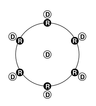
Figure 31: The ideal case with $N$ reactors (R) and $(N+1)$ detectors (D).

In this case the effective systematic error becomes

$$\displaystyle\sigma_{eff}^{2}={\left(1+1/N\right)\sigma_{u}^{2}\over 1+(1/N)\left\{1+(N+1)\left[\sigma_{c}^{2}+(\sigma^{(r)}_{c})^{2}+(\sigma^{(r)}_{u})^{2}/N\right]/\sigma_{u}^{2}\right\}^{-1}},$$ (22)

where the conditions $T^{F}_{a}=T^{F}/N$ and $T^{Nb}_{a}=\delta_{a}^{b}\,T^{Nb}$ have been assumed; $T^{F}_{a}$ and $T^{Nb}_{a}$ are the yield at the far and $b$-th near detector which is close to the $b$-th reactor ($b=1,\cdots,N$) from the $a$-th reactor, and $T^{F}$ and $T^{Nb}$ are the total yield at the far and $b$-th near detector. As in the case with one reactor, the dominant contribution to $\sigma_{eff}$ comes from the uncorrelated error $\sigma_{u}$, and the contribution of the uncorrelated error $\sigma^{(r)}_{u}$ is reduced in (22) by a factor of $N$ due to the averaging over the independent $N$ fluctuations, but this reduction is irrelevant because such an effect comes in the correlated error which is almost canceled in the multi detector system. To conclude, the answer to the question at the beginning of this section is that the cancellation of the correlated error occurs also in the ideal case with $N$ reactors and $(N+1)$ detectors. It should be noted that the number $N$ of the near detectors in this case is sufficient but not necessary to guarantee this cancellation, as we will see below in the case of the Kashiwazaki plan.

8.4.4 Kashiwazaki case study

The next question which arises is: what happens to the cancellation of the correlated error in the Kashiwazaki plan. The Kashiwazaki-Kariwa nuclear plant consists of two clusters of reactors, and one cluster consists of four reactors while the other consists of three (See Figure 32).

Figure 32: The Kashiwazaki plan with 7 reactors (R) and 3 detectors (D).

Figure 33: The ideal limit of the Kashiwazaki plan, where one reactor has the power four times as much as one of the Kashiwazaki-Kariwa reactors, while the other has the power three times as much as that of the KK reactors.

Before we discuss the effective systematic error for the actual Kashiwazaki plan, let us consider the ideal limit, where the cluster of the four reactors shrinks to one reactor and the other of three reactors shrinks to another single reactor (See Figure 33). It can be shown analytically that the effective systematic error for this ideal limit is given by

$$\displaystyle\sigma_{eff}\simeq{\sqrt{74}\over 7}\,\sigma_{u},$$

where the correlated error has been canceled due to the near-far detector complex, and the reason that we have the factor $\sqrt{74/49}$ instead of $(1+1/N)^{1/2}|_{N=2}=\sqrt{3/2}$ is because the yield from the first reactor to that from the second is 4:3 instead of 1:1. Thus we see that the cancellation of the correlated errors occurs also in the ideal limit of the Kashiwazaki plan. Furthermore, it can be shown from the numerical calculations that the difference between $\sigma_{eff}$ for the actual Kashiwazaki plan and that for the ideal limit is very small:

$$\displaystyle{\left.\sigma_{eff}\right|_{actual~{}KK}\over\left.\sigma_{eff}\right|_{ideal~{}KK}}=1.04,$$

where $\sigma_{u}=0.6\%$, $\sigma_{c}=1.6\%$, $\sigma^{(r)}_{u}=2.3\%$, $\sigma^{(r)}_{c}=2.5\%$ have been used as reference values for the systematic errors. This shows that the cancellation of the correlated errors occurs also in the actual Kashiwazaki plan.

The systematic limit on $\sin^{2}2\theta_{13}$ at 90%CL can be obtained from the effective systematic error by

$$\left(\sin^{2}2\theta\right)_{limit}^{sys~{}only}={\sqrt{2.7}\,\sigma_{eff}\over\mbox{"}\left\langle\sin^{2}\left({\Delta m^{2}L_{far}\over 4E}\right)\right\rangle\mbox{"}-\mbox{"}\left\langle\sin^{2}\left({\Delta m^{2}L_{near}\over 4E}\right)\right\rangle\mbox{"}},$$ (23)

where

$$\displaystyle\mbox{"}\left\langle\sin^{2}\left({\Delta m^{2}L_{far}\over 4E}\right)\right\rangle\mbox{"} \equiv \displaystyle\sum_{a=1}^{7}\omega^{far}_{a}\left\langle\sin^{2}\left({\Delta m^{2}L^{far}_{a}\over 4E}\right)\right\rangle,$$

$$\mbox{"}\left\langle\sin^{2}\left({\Delta m^{2}L_{near}\over 4E}\right)\right\rangle\mbox{"} \equiv \displaystyle{4\over 7}\sum_{a=1}^{7}\omega^{near-1}_{a}\left\langle\sin^{2}\left({\Delta m^{2}L^{near-1}_{a}\over 4E}\right)\right\rangle$$

$$+ \displaystyle{3\over 7}\sum_{a=1}^{7}\omega^{near-2}_{a}\left\langle\sin^{2}\left({\Delta m^{2}L^{near-2}_{a}\over 4E}\right)\right\rangle,$$

stands for the averaged expectation value of the factor $\sin^{2}\left({\Delta m^{2}L/4E}\right)$, $L^{X}_{a}$ ($X$=near-1, near-2, far) is the distance between the detector $X$ and the $a$-th reactor ($a=1,\cdots,7$), and $\omega^{X}_{a}$ ($X$=near-1, near-2, far) is the fraction of the yield from the $a$-th reactor at the detector $X$ (=(power of $a$-th reactor)/$(L^{X}_{a})^{2}$). The expectation $\left\langle\cdots\right\rangle$ is defined by

$$\displaystyle\left\langle\sin^{2}\left({\Delta m^{2}L\over 4E}\right)\right\rangle \equiv {\displaystyle\int dE~{}\epsilon(E)f(E)\sigma(E)\sin^{2}\left({\Delta m^{2}L\over 4E}\right)\over\displaystyle\int dE~{}\epsilon(E)f(E)\sigma(E)},$$

where $\epsilon(E)$, $f(E)$, $\sigma(E)$ stand for the detection efficiency, the neutrino flux, and the cross section, respectively. If $|\Delta m^{2}_{31}|=2.5\times 10^{-3}$eV², then we have

$$\mbox{"}\left\langle\sin^{2}\left({\Delta m^{2}L_{far}\over 4E}\right)\right\rangle\mbox{"}=0.70$$

$$\mbox{"}\left\langle\sin^{2}\left({\Delta m^{2}L_{near}\over 4E}\right)\right\rangle\mbox{"}=0.17$$

in the setup of the Kashiwazaki plan. So, if $\sigma_{u}$=0.6%, then Equation (23) becomes

$$\left(\sin^{2}2\theta\right)_{limit}^{sys~{}only}={\sqrt{2.7}\over 0.53}{\sqrt{74}\over 7}0.006=0.022.$$

Furthermore, if we include the statistical error $\sigma_{stat}=1/\sqrt{60,000}$ in the case of 20 t$\cdot$yr, then we get

$$\left(\sin^{2}2\theta\right)_{limit}^{sys~{}only}={\sqrt{2.7}\over 0.53}\sqrt{(74/49)0.006^{2}+1/60,000}=0.025.$$

Figure 34: (a) Comparison of the actual Kashiwazaki plan (the solid line) and a hypothetical experiment (the dashed line), which is depicted in Figure 35, with a single 24.3$GW_{th}$ reactor and two detectors assuming the same uncorrelated systematic error $\sigma_{u}$. (b) Comparison of the actual Kashiwazaki plan (the solid line) and a hypothetical experiment (the dashed line), which is depicted in Figure 36, where the near detectors are placed in wrong location. The statistical errors as well as all the systematic errors except $\sigma^{(r)}_{u}$, which is assumed to be 2.3%, are ignored for simplicity.

In Figure 34(a) comparison is given between the actual Kashiwazaki plan and a hypothetical experiment, which is depicted in Figure 35, with a single reactor and two detectors, where the same uncorrelated systematic error $\sigma_{u}$ and the same data size (=20t$\cdot$yr) are assumed (Only in this figure the statistical errors are taken into account).

Figure 35: The case where a single reactor has the power seven times as much as one of the Kashiwazaki-Kariwa nuclear plant.

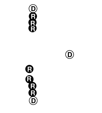
Figure 36: A hypothetical experiment with the same location of the reactors as the Kashiwazaki plan but with stupid location of the near detectors.

We observe that there is little difference between the sensitivities of the actual Kashiwazaki plan and the hypothetical experiment with a single reactor at $|\Delta m^{2}_{31}|=2.5\times 10^{-3}$eV². Also it is remarkable that the sensitivity of the actual Kashiwazaki plan for higher value of $|\Delta m^{2}_{31}|$ is better than the single reactor experiment. This is exactly because of the reduction of the uncorrelated error due to the nature of multiple reactors (cf. Equation (21)), where the near detectors play a role as far detectors. On the other hand, to see how effectively the correlated errors are canceled in the actual Kashiwazaki plan, comparison is given in Figure 34(b) between the locations of the near detectors in the actual Kashiwazaki plan and a hypothetical plan which is depicted in Figure 36, with one near detector very close to reactor #1 in the first cluster while the other detector is very close to reactor #5 in the second. In the hypothetical case, the sensitivity is deteriorated because the correlated errors do not cancel completely. From these two figures we see that the setup of the Kashiwazaki plan is almost optimized and it does not suffer from an extra uncertainty because there are more than one reactors.

8.4.5 Energy spectrum analysis [102]

One can also derive a semi-analytic formula for the effective systematic error in the analysis of the energy spectrum, assuming that the uncorrelated bin-to-bin error $\sigma_{u}$ is independent of bin. The result is

$$\displaystyle\sigma_{eff}^{2}={{a_{n}\over n}\,\sigma_{u}^{2}\over\left[1+{\sigma_{u}^{2}\over\sigma_{u}^{2}+2\sigma_{shape}^{2}}+b_{n}\left({\sigma_{u}^{2}\over\sigma_{u}^{2}+n\sigma_{c}^{2}}+{\sigma_{u}^{2}\over\sigma_{u}^{2}+2\sigma_{shape}^{2}+n\sigma_{c}^{2}+2n(\sigma^{(r)})^{2}}\right)\right]},$$

where $n$ stands for the number of bins, $\sigma_{c}$ is the total correlated error, $\sigma_{shape}$ is an uncertainty of the theoretical prediction for each energy bin which is uncorrelated between different energy bins, $\sigma^{(r)}$ is the uncertainty of the flux, and the error of the energy calibration has been ignored because it turns out to be small. $a_{n}$ and $b_{n}$ are given by

$$a_{n} \equiv {2\over f_{n}}$$

$$b_{n} \equiv {g_{n}\over f_{n}}$$

$$f_{n} \equiv \displaystyle{1\over n}\sum_{j=1}^{n-1}{1\over j(j+1)}\left(\sum_{k=1}^{j}c_{k}-(j+1)c_{j}\right)^{2}$$

$$g_{n} \equiv {1\over n^{2}}\left(\displaystyle\sum_{j=1}^{n}c_{j}\right)^{2}$$

$$c_{j} \equiv \left\langle\sin^{2}\left({\Delta m^{2}L_{far}\over 4E_{j}}\right)\right\rangle\quad(j=1,\cdots,n),$$

and their numerical values are given in Table 10. The integration over the energy in the expectation value to define $c_{j}$ is from $E_{j}$ to $E_{j+1}$. The systematic limit on $\sin^{2}2\theta_{13}$ at 90%CL is obtained from $\sigma_{eff}$ by

$$\left(\sin^{2}2\theta\right)_{limit}^{sys~{}only}=\sqrt{2.7}\,\sigma_{eff}.$$

For simplicity let us assume $\sigma_{shape}=0$ and $\sqrt{n}\sigma^{(r)}\gg\sqrt{n}\sigma_{c},~{}\sigma_{u}$. Then we have

$$\sigma_{eff}=\sqrt{{a_{n}\over 2n}}\,\sigma_{u}\left(1+{b_{n}\over 2}{\sigma_{u}^{2}\over\sigma_{u}^{2}+n\sigma_{c}^{2}}\right)^{-1/2}.$$ (24)

If we further assume $\sigma_{u}=\sigma_{c}$ then (24) is reduced to

$$\sigma_{eff}=\sqrt{{a_{n}\over 2n}}\,\sigma_{u}\left(1+{b_{n}\over 2n+2}\right)^{-1/2},$$

and the numerical values of ${b_{n}/(2n+2)}$ are given in Table 11, which shows that the contribution of the correlated error is not negligible for lower value of $n$. On the other hand, if we assume $\sqrt{n}\sigma_{c}\gg\sigma_{u}$, then we have

$$\sigma_{eff}=\sqrt{{a_{n}\over 2n}}\,\sigma_{u},$$

and it indicates that the uncorrelated error gives the dominant contribution to the effective systematic error. The same conclusion is reached if $\sqrt{n}\sigma_{c}\ll\sigma_{u}$ is assumed. Therefore the realistic value of the uncorrelated bin-to-bin error $\sigma_{u}$ has to be estimated carefully in any case.

n	$a_{n}$	$b_{n}$
2	151	44
4	76	20
6	60	15
6	51	12
16	41	10
$\geq 30$	$\sim$ 40	$\sim$ 9

Table 10: The coefficients $a_{n}$ and $b_{n}$ which were calculated numerically.

n	$(a_{n}/2n)^{1/2}$	$b_{n}/(2n+2)$
2	6.2	7.3
4	3.1	2.0
6	2.2	1.1
6	1.8	0.7
16	1.1	0.3
62	0.6	0.1

Table 11: The numerical values of the coefficients $(a_{n}/2n)^{1/2}$ and $b_{n}/(2n+2)$ which appear in $\sigma_{eff}$ in the case of $\sigma_{c}=\sigma_{u}$.

9 Possible Sites

In this section we examine the power performance of commercial reactor sites all over the world and summarize the assets of sites that have been identified as candidates to host a $\sin^{2}2\theta_{13}$ experiment.

Site selection will involve a comprehensive look at many criteria such as potential for earth shielding, locations for near and far detectors, construction costs and reactor power. Ultimately, choosing a site will require a a comparison of cost and sensitivity for site specific proposals.

9.1 Top Performing Reactors Worldwide

One characteristic on which various reactor sites can be directly compared is power. Tables 12, 13 and 14 list maximum and average power output for single, double and multi-reactor sites respectively. The reactor sites are sorted by their average power output as measured over the 7 year period from 1996 to 2002. The maximum rated power of each site is also listed. Sites with maximum power ratings of less then 3 GW per reactor core (or 9 GW for multi-reactor sites) are considered only if they have been identified as potential host sites.

Reactor Site Country Avg $MW_{th}$ Max $MW_{th}$ Brokdorf Germany 3900 4214 Emsland Germany 3892 4097 Grohnde Germany 3858 4184 Grand Gulf US 3505 3833 Grafenrheinfeld Germany 3357 3936 Wolf Creek US 3211 3565 Perry US 3199 3758 Callaway US 3176 3565 Leibstadt Switzerland 3130 3511 Waterford US 3152 3390 Watts Bar US 3049 3411 Unterweser Germany 3117 4126 Seabrook US 2924 3411 Vandellos Spain 2882 3181 Kruemmel Germany 2868 3851 Confrentes Spain 2858 3160 Hope Creek US 2794 3339 Fermi US 2750 3430 River Bend US 2676 3039 Trillo Spain 2672 3119 Columbia US 2567 3486 Tokai Japan 2086 3219 Krasnoyarsk Russia 1600(?) 2000(?)

Table 12: Power performance for single reactor sites around the world [103, 104].

Reactor Site Country Avg $MW_{th}$ Max $MW_{th}$ South Texas Project US 6864 7600 Civaux France 6799 9135 Chooz France 6795 8872 Gundremmingen Germany 6734 7865 Braidwood US 6491 7172 Vogtle US 6456 7130 Byron US 6442 7172 Browns Ferry US 6377 6916 Limerick US 6365 6916 Isar Germany 6313 6985 Peach Bottom US 6290 6916 Sequoyah US 6209 6822 Penly France 6197 8088 Philippsburg Germany 6187 6976 Susquehanna US 6161 6978 Golfech France 6136 7977 Catawba US 6116 6822 Nogent France 6111 7977 San Onofre US 6061 6876 Diablo Canyon US 6043 6749 Comanche Peak US 5986 6916 St. Alban/St. Maurice France 5910 8082 Neckar Germany 5881 6452 McGuire US 5880 6822 Flamanville France 5879 8088 Biblis Germany 5528 7388 Asco Spain 5496 6013 Belleville France 5377 7977 Kuo-Sheng Taiwan 4749 5764 Angra Brazil 4547 5873 Indian Point US 4467 6096 La Salle US 4323 6978 Salem US 4281 6918 Ignalina Lithuania 3985 8778 D.C. Cook US 3281 6661 Millstone US 3271 6111

Table 13: Power performance for double reactor sites around the world [103, 104].

Reactor Site Country Cores Avg $MW_{th}$ Max $MW_{th}$ Kashiwazaki-Kariwa Japan 7 20302 24029 Yonggwang S. Korea 6 16393 17264 Gravelines France 6 12458 16696 Zaporozhe Ukraine 6 12202 17557 Catternom France 4 12113 15942 Paluel France 4 11901 16176 Ohi Japan 4 11269 13782 Palo Verde US 3 10570 11552 Fukushima II Japan 4 10384 12875 Fukushima I Japan 6 10181 13741 Darlington Canada 4 9028 10932 Chinon France 4 8653 11166 Blayais France 4 8644 11131 Cruas France 4 8586 11190 Takahama Japan 4 8439 9925 Genkai Japan 4 8330 10177 Kori S. Korea 4 8314 9203 Ringhals Sweden 4 8307 10841 Tricastin France 4 8284 11178 Bruce Canada 4 8080 10710 Tihange Belgium 3 8075 9127 Hamaoka Japan 4 8031 10584 Forsmark Sweden 3 7773 9408 Dampierre France 4 7753 10967 Bugey France 4 7728 10897 Leningrad Russia 4 7642 11705 Balakovo Russia 4 7520 11705 Kozloduy Bulgaria 6 6618 11002 Kursk Russia 4 6577 11705

Table 14: Power performance for multi-reactor sites around the world [103, 104].

9.2 Reactors Sites Under Consideration

Many possible host reactor sites have been identified by groups around the world. In this section we list some of the relevant features from each site mentioned for consideration.

9.2.1 Angra, Brazil

The Angra reactors are located on the coast of Brazil a few hours south of Rio de Janeiro. The site is ringed by sharply rising hill on three sides, with summits of over 200 meters within 1.5 km.

The president of the reactor company is a former particle physicist and groups at several Brazilian institutions have shown an interest.

9.2.2 Braidwood, Byron and La Salle, Illinois

These reactor sites are all located within 100 km of both Fermilab and Argonne National Laboratory, making them easily accessible to the particle physics community. The topology of northern Illinois is generally flat, so obtaining cosmic shielding at these sites will require extensive excavation below the surface level. Fortunately, the subterranean geology of this region is well understood [105]. At the Braidwood and La Salle sites there is a layer of dolomite, which is well suited for excavation, at a depth of 110 meters (approximately 300 mwe). At the Byron site, the western most of the three, the dolomite layer is much closer to surface. Below the dolomite, starting at a depth of 50 to 100 meters, is a layer of sandstone, which may be poorly suited for supporting excavated cavities.

The Braidwood, Byron and La Salle reactors are owned and operated by the Exelon Corporation. Currently, negotiations are ongoing with Exelon for the use of these sites.

9.2.3 Chooz, France

This is the location of the previous 10 ton CHOOZ experiment, and a site for a new near detector has been identified near the reactors. The CHOOZ plant has a total 8.4 thermal GW and the CHOOZ-far lab is located 1.05 km from the two cores.

9.2.4 Cruas, France

The Cruas site is located in south eastern France. The most likely near detector baseline is about 1 km with a shielding potential of greater than 200 mwe. A far detector located at 1.8 km could get shielding greater than 400 mwe.

9.2.5 Daya Bay, China

There are two twin reactor cores located in Guangdong province near Hong Kong. The total reactor power is 11.6 GW. A third twin core is planned to be online in 2010. A near hall with an overburden of 400 mwe is potentially located about 300 m from the core, and a far hall with 1200 mwe at a distance of 1500-2000 m to the core.

9.2.6 Diablo Canyon, California

The Diablo Canyon site is located on the coast of California. Within 1.5  km of the reactors are hills of over 300 meters. All the surrounding land is owned by the utility, PG&E, with which negotiations for the use of the site are ongoing.

9.2.7 Kashiwazaki-Kariwa, Japan

The Kashiwazaki-Kariwa reactor complex is the most powerful in the world. The site consists of 7 active reactors spanning approximately 700 meters. The site is relatively flat, so detectors would be located at the bottom of vertical shafts. Permission for the use of the site has been granted by the power company. A full description of a proposal at this site is given in Appendix A.

9.2.8 Krasnoyarsk, Russia

The Krasnoyarsk reactor is part of a fully underground facility at a depth of 600 mwe. Halls suitable for detectors exist at baselines of 115 meters and 1000 meters. Like the Wolf Creek site this single reactor site will allow for a sensitive determination of the background rate.

Russian physicists have a long-standing relationship with the facility and have mounted several neutrino experiments in the past [106].

9.2.9 Kuo-Sheng, Taiwan

The Kuo-Sheng reactor complex is located in a hilly region of coastal Taiwan. The existence of a road tunnel within 2 km of the reactor indicates that tunneling is viable in the hills surrounding the site. Within 500 meters of the reactor there are hills 50 meters or higher suitable for shielding a near detector. Far detector shielding of 150 to 200 meters of rock is possible.

Local physicists have an existing relationship with the reactor operators and are currently operating a neutrino magnetic moment experiment at a distance of 28 meters from one of the two reactor cores [107].

9.2.10 Limerick and Peach Bottom, Pennsylvania

These reactor sites are also owned and operated by Exelon. The topology of Pennsylvania is somewhat more hilly than in Illinois. Therefore, the potential for significant earth shielding with horizontal access may exist at these sites. In particular, Peach Bottom has elevation variations of greater that 60 meters within 1.5 km of the reactors.

9.2.11 Penly, France

The Penly reactor complex is embedded in 120 meter high chalk cliffs.

9.2.12 Wolf Creek, Kansas

The topology of this single reactor site is similar to the flat sites in Illinois. At a depth of 110 meters there is relatively wide layer of shale. While the shale is not ideal for tunneling it is likely sufficient to support the structures required for this project.

The main attraction of the Wolf Creek site is that as a single reactor facility it will get full reactor off running which can be used to measure the background rate.

10 Other physics

The main goal of the experiment described in this white paper is to search for or further limit the value of $\theta_{13}$. It is reasonable to explore whether there is other physics that can be done with this experiment, or with modest enhancements. In this section we briefly consider three other physics topics: sterile neutrinos, $\theta_{12}$ and reactor physics.

10.1 Sterile Neutrinos

The discovery of sterile neutrinos would have a revolutionary impact on neutrino and particle physics. If there is non-negligible mixing of the electron neutrino with sterile neutrinos, they would contribute to the reactor antineutrino disappearance pattern. An idea how to look for sterile neutrinos at reactors along with $\sin{\theta}_{13}$ was proposed at the Kurchatov Institute in 1998 [108].

The notion of sterile neutrinos was originally introduced by B. Pontecorvo in 1967 [109] and has been considered later by many authors, e.g., D. Caldwell and R. Mohapatra [110], J.T. Peltoniemi, D. Tommasini and J.W.F. Valle [111], S. Bilenky, C. Giunti and W. Grimus [112], K. Benakli and A. Smirnov [113], B. Kayser [114]. Information on the theory of sterile (and mirror) neutrinos and references can be found in the recent paper by V. Berezinsky, M. Narayan, F. Vissani [115].

While solar, atmospheric, and laboratory (Super Kamiokande, SNO, KamLAND) studies are understood in the framework of only 3-active neutrino mixing (see, however, de Holanda and Smirnov [116]) they do not exclude some admixture of sterile neutrinos [1]. An experimental hint in favor of sterile neutrinos comes from the unconfirmed observation of the LSND collaboration [118] on ${\nu}_{\mu}\rightarrow{\nu}_{e}$ transitions. In particular the so-called (3+1) and (3+2) neutrino schemes, which have been considered to explain the LSND signal, predict reactor neutrino disappearance with a $\Delta m^{2}\sim$ eV² very close to the current upper bound from the Bugey experiment (see References [119] and [120]).

10.1.1 The effect of sterile neutrinos in $\theta_{13}$ reactor experiments

In the standard 3-active neutrino framework, antineutrino disappearance at distances $L=1000-2000$ m from a reactor source is governed by $\Delta m^{2}_{\mathrm{atm}}\sim 2\times 10^{-3}$ eV² and by the mixing parameter $\sin^{2}2\theta_{13}$:

$$P_{\bar{\nu}_{e}\rightarrow\bar{\nu}_{e}}\approx 1-\sin^{2}2{\theta}_{13}\,\sin^{2}\left(\frac{\Delta m^{2}_{\mathrm{atm}}L}{4E}\right)\,.$$ (25)

Let us denote the three standard neutrino mass states by $\nu_{i}$ ($i=1,2,3$), such that the atmospheric and solar mass-squared differences are given by $\Delta m^{2}_{\mathrm{atm}}=m^{2}_{3}-m_{1}^{2}$ and $\Delta m^{2}_{\mathrm{sol}}=m^{2}_{2}-m_{1}^{2}\sim 7\times 10^{-5}$ eV², the solar mixing angle is determined by $\tan^{2}\theta_{\mathrm{sol}}=|U_{e2}|^{2}/|U_{e1}|^{2}\sim 0.4$, and $\sin^{2}2\theta_{13}=4|U_{e3}|^{2}(1-|U_{e3}|^{2})$. If we now assume that there are additional neutrino states $\nu_{i}$ ($i=4,5,\ldots$) with masses such that $|\Delta m^{2}_{i1}|\>\raisebox{-2.15277pt}{$\stackrel{{\scriptstyle\textstyle>}}{{\sim}}$}\>10^{-3}$ eV² we know from the Bugey, Palo Verde and CHOOZ experiments that the mixing of the electron neutrino with these new mass states has to be small (see shaded region in Figure 38), i.e.,

$$|U_{ei}|^{2}\ll 1\quad\mbox{for}\quad i\geq 3\,.$$ (26)

To first order in these small quantities one obtains for the survival probability at nuclear reactors

$$P_{\bar{\nu}_{e}\rightarrow\bar{\nu}_{e}}\approx 1-4\sum_{i\geq 3}|U_{ei}|^{2}\,\sin^{2}\left(\frac{\Delta m^{2}_{i1}L}{4E}\right)\,.$$ (27)

In the case of only one additional neutrino one can write Equation (27) as

$$P_{\bar{\nu}_{e}\rightarrow\bar{\nu}_{e}}\approx 1-\sin^{2}2{\theta}_{13}\,\sin^{2}\left(\frac{\Delta m^{2}_{\mathrm{atm}}L}{4E}\right)-\sin^{2}2{\theta}_{s}\,\sin^{2}\left(\frac{\Delta m^{2}_{\mathrm{new}}L}{4E}\right)\,,$$ (28)

where $\sin^{2}2{\theta}_{s}\approx 4|U_{e4}|^{2}$ and $\Delta m^{2}_{\mathrm{new}}=m_{4}^{2}-m_{1}^{2}$ are the mixing parameters of the sterile neutrino, and $\sin^{2}2{\theta}_{13}\approx 4|U_{e3}|^{2}$.

From Equation (28) it is obvious that such a sterile neutrino would have some impact on an experiment of the Kr2Det type [121] or its modifications (as discussed in 2002–2003 at the meetings in Paris, Alabama and Munich), provided the associated mixing parameter $\sin^{2}2{\theta}_{s}$ is not too small and the mass-splitting is in the relevant range.

• If $\Delta m^{2}_{\mathrm{new}}\sim\Delta m^{2}_{\mathrm{atm}}$ it will be rather difficult to disentangle $\bar{\nu}_{e}\to\bar{\nu}_{\mu/\tau}$ oscillations with $\sin^{2}2\theta_{13}$ from $\bar{\nu}_{e}\to\bar{\nu}_{s}$ oscillations with $\sin^{2}2\theta_{s}$ at a reactor experiment, especially if the main information comes from the total rate measurement. Only if enough spectral information is available and/or $\Delta m^{2}_{\mathrm{atm}}$ and $\Delta m^{2}_{\mathrm{new}}$ differ sufficiently one might be able to separate the two channels. If no effect is observed both, $\sin^{2}2\theta_{13}$ and $\sin^{2}2\theta_{s}$ can be constrained.

• If $\Delta m^{2}_{\mathrm{new}}\gg\Delta m^{2}_{\mathrm{atm}}$ and the oscillations with $\Delta m^{2}_{\mathrm{new}}$ are already averaged out at the near detector position at $L\sim$ few $\times 100$ m, no information about sterile neutrino mixing can be obtained from the comparison of the far and near detectors, and the transitions to the sterile state will not affect the $\theta_{13}$ measurement. In that case information on sterile neutrino mixing can be obtained from the near detector if relatively precise information on the initial reactor neutrino flux is available, or if a “very-near” detector at $L\sim 10$ m could be installed (see below).

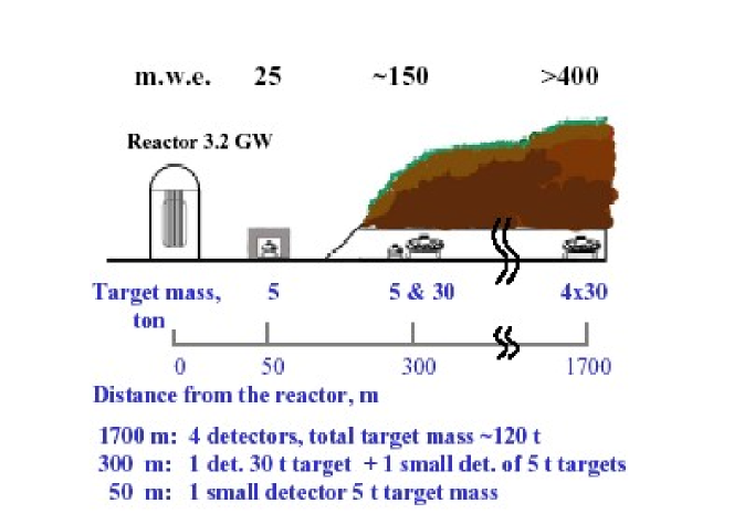
Figure 37: Example of a layout. Detector positions, target scintillator masses and overburden (m.w.e.) are shown.

10.1.2 Example of layout

Imagine that a tunnel is built near one 3.2 GW thermal power reactor. We consider five identically designed 30 ton target scintillator (movable) detectors, four of them stationed in the far position at a distance of 1700 m from the reactor, and one detector stationed in the near position at 300 m from the reactor. To expand the explored mass parameter region toward larger values two small detectors are considered at 300 m and 50 m from the reactor. A possible layout of such an experiment is illustrated in Figure 37. The expected neutrino detection rates per 300 days are shown in Table 15.

Distance [m]	Target mass [t]	$\bar{\nu}_{e}$ rate/300day
50	5	1 100 000
300	5	30 000
300	30	190 000
1700	4 x 30	24 000

Table 15: Detector positions, scintillator target masses and $\bar{\nu}_{e}$ detection rates per 300 days.

We consider two types of data analysis: shape and rate. With only one reactor as $\bar{\nu}_{e}$ source the shape analysis (as we already know) is independent of the exact knowledge of reactor power, energy spectrum of the $\bar{\nu}_{e}$, flux and spectral time variations, target volumes and proton concentrations, and absolute efficiencies of $\bar{\nu}_{e}$ detection. Backgrounds can be measured periodically during reactor-off periods. On the other hand, the analysis based on the comparison of the far/near $\bar{\nu}_{e}$ total rates requires good knowledge of the ratios of target volumes and detection efficiencies. In both cases no exact information from the reactor services on reactor power and fissile fuel composition is needed for the data analysis.

10.1.3 Sensitivity

In Figure 38 we show the sensitivity for $\sin^{2}2\theta_{13/s}$ for the experimental configuration described in the previous section. Within 3 years of data taking (300 days/year) in a large part of the $\Delta m^{2}$ range from 0.001 to 0.5 eV² a sensitivity of $\sin^{2}2{\theta}_{13/s}\sim 0.01-0.02$ can be obtained [122], which is in general agreement with the analysis performed by P. Huber, M. Lindner, T. Schwetz and W. Winter [30]. The limits shown in Figure 38 were obtained by assuming an energy resolution ${\sigma}_{E}=0.08\sqrt{E}$ and the systematics ${\sigma}_{\mathrm{shape}}=0.5\%,{\sigma}_{\mathrm{rate}}=1\%$. As can be seen in the figure the CHOOZ limit on $\sin^{2}2{\theta}_{13}$ at ${\Delta}m^{2}_{\mathrm{atm}}=2\times 10^{-3}$ eV² can be improved by a factor 10.

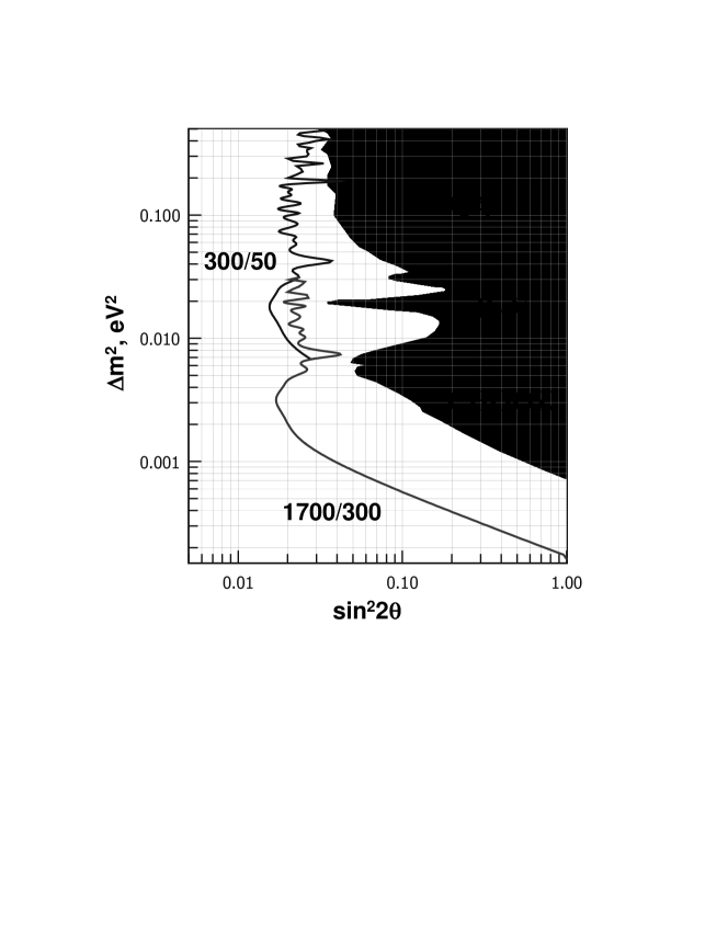
Figure 38: Expected 90% CL limits from the comparison of detectors at distances of 300/1700 m and 50/300 m. The shaded region is excluded by the CHOOZ, Palo Verde and Bugey experiments.

We conclude that a search for sterile neutrinos at reactors does not require much additional effort and can be done along with ${\theta}_{13}$. With one reactor and a number of detectors a high sensitivity to ${\theta}_{13}$ and sterile neutrino mixing can be reached. To increase the sensitivity in the range $\Delta m^{2}\gg\Delta m^{2}_{\mathrm{atm}}$ [in particular to reach the $\mathcal{O}$(eV²) region indicated by the LSND evidence] a very-near detector at $L\sim 10$ m is necessary.

10.2 Solar Neutrinos and $\theta_{12}$

10.2.1 The present and near-future for $\theta_{12}$

The first data from the KamLAND experiment [7] showed that the reactor $\bar{\nu}_{e}$ undergo oscillations on a distance scale of  $\sim 160$ km. Under the plausible assumption of CPT-invariance, this result confirmed the Large Mixing Angle (LMA) solution of the solar neutrino ($\nu_{\odot}$) problem. When combined with the solar neutrino data, the KamLAND data split the allowed LMA solution region of $\nu_{\odot}$ oscillation parameters $\Delta m^{2}_{21}$ and $\sin^{2}\theta_{12}$ into two sub-regions – low-LMA and high-LMA. The best fit values of $\Delta m^{2}_{21}$ and $\sin^{2}\theta_{12}$ in the two sub-regions read: $\Delta m^{2}_{21}=7.2\times 10^{-5}$ eV², $\sin^{2}\theta_{12}=0.3$ (low-LMA), and $\Delta m^{2}_{21}=1.5\times 10^{-4}$ eV², $\sin^{2}\theta_{12}=0.3$ (high-LMA) [124]. Adding the salt phase data from the SNO experiment [6] the global analysis allows the high-LMA solution only at the 99.13% CL [125]. Thus, the high-LMA solution is disfavored by the current data compared to the low-LMA one, although it is still not ruled out comprehensively.

The $\bar{\nu}_{e}$ survival probability in the reactor experiments of interest, $P_{ee}$, depends on $\Delta m^{2}_{21}$, $\sin^{2}\theta_{12}$, $\Delta m^{2}_{31}$ (driving the atmospheric neutrino oscillations), the angle $\theta_{13}$ limited by the CHOOZ and Palo Verde experiments, and on the type of neutrino mass hierarchy [126, 127]. The potential sensitivity of a reactor experiment to each of these parameters depends crucially on the baseline of the experiment. Experiments with a baseline $L\sim(1-2)$ km can be used to get information on $\sin^{2}\theta_{13}$: on the indicated distances only oscillations induced by $\Delta m^{2}_{31}$ are operative and $\sin^{2}2\theta_{13}$ determines their amplitude. For baselines $L\ \raisebox{-1.72218pt}{\hbox to0.0pt{$\sim$\hss}}\raisebox{1.72218pt}{$>$}\ 50$ km, the $\bar{\nu}_{e}$ oscillations due to $\Delta m^{2}_{31}$ average out and we have: $P_{ee}\approx[1-\sin^{2}2\theta_{12}\sin^{2}(\Delta m^{2}L/4E)]\cos^{4}\theta_{13}$. The oscillations generated by $\Delta m^{2}_{21}$ have been seemingly detected in the KamLAND experiment.

In the absence of oscillations, the maximal contribution to the signal in an experiment with reactor $\bar{\nu}_{e}$ detected via the inverse $\beta-$decay reaction comes from $\bar{\nu}_{e}$ with energy $E\sim 3.6$ MeV. For a fixed $\Delta m^{2}_{21}$, maximal sensitivity to $\sin^{2}\theta_{12}$ can be achieved if for $E\sim 3.6$ MeV, $L$ is “tuned” to a $\bar{\nu}_{e}$ survival probability minimum (SPMIN), i.e., if $\sin^{2}(\Delta m^{2}L/4E)\approx 1$. The latter is reflected in the $e^{+}-$spectrum, measured in the experiment. The corresponding minimum in the spectrum is determined by $P_{ee}\approx 1-\sin^{2}2\theta_{12}$, and thus is very sensitive to the value of $\sin^{2}2\theta_{12}$. If, in contrast, $L$ is such that $\sin^{2}(\Delta m^{2}L/4E)=\epsilon\ll 1$, $P_{ee}$ would have a maximum (SPMAX): $P_{ee}\approx 1-\epsilon\sin^{2}2\theta_{12}\approx 1$. In this case the sensitivity to $\sin^{2}2\theta_{12}$ is worse than in the preceding one. The positions of the extrema in both cases are highly sensitive to the value of $\Delta m^{2}_{21}$.

For values of $\Delta m^{2}_{21}$ from the low-LMA region, $\Delta m^{2}_{21}\sim 7.2\times 10^{-5}$ eV², and $E\sim 3.6$ MeV, the SPMIN and SPMAX take place at $L\sim 70$ km and $L~{}\sim~{}160$ km. For the KamLAND experiment, the most powerful reactors (the Kashiwazaki complex) are located at a distance of $\sim 160$ km, unfortunately close to the SPMAX for low-LMA. The values of $\Delta m^{2}_{21}$ and $\sin^{2}\theta_{12}$, allowed at 99% CL by existing and prospective KamLAND data have been determined in References [128, 129]. The uncertainty in $\Delta m^{2}_{21}$, determined using only the $\nu_{\odot}$ data, reduces from 68% to 30% after the inclusion of the first KamLAND data in the analysis, while that in $\sin^{2}\theta_{12}$ does not change, remaining rather large (29%). The uncertainty in $\Delta m^{2}_{21}$ would further diminish to 9% (6%) after 1 kTy (3 kTy) data from KamLAND. However, there will be little improvement in the precision on the value of $\sin^{2}\theta_{12}$ with the increase of KamLAND statistics.

The $L$ best suited for measuring $\theta_{12}$ if $\Delta m^{2}_{21}$ lies in the low-LMA region is $\sim 70$ km [128]. For a reactor complex with a power of 24.6 GW (e.g., Kashiwazaki) and data of 3 kTy from a KamLAND-like detector at $L\sim 70$ km, $\sin^{2}\theta_{12}$ can be determined at 99% CL with a $\sim$10% uncertainty [128].

A new reactor power plant, Shika-2, is expected to start operations in Japan in March 2006. It will be located at $L\sim 88$ km from KamLAND and will have a power of $\sim$4 GW. This baseline is close to the “ideal” one of $L\sim 70$ km. The implications of the new source of $\bar{\nu}_{e}$ on the KamLAND sensitivity to $\Delta m^{2}_{21}$ and $\sin^{2}\theta_{12}$ were studied in [130]. It was concluded that due to averaging effects of the ${\bar{\nu}_{e}}$ fluxes from the Kashiwazaki and Shika-2 reactors, the sensitivity of KamLAND to $\sin^{2}\theta_{12}$ would not improve, while its sensitivity to $\Delta m^{2}$ would diminish.

If contrary to the trend emerging in the solar neutrino experiments the next KamLAND results conform to a point in the high-LMA region, one would need an intermediate baseline reactor experiment with $L\sim(20-30)$ km to get a SPMIN in the resultant $e^{+}-$spectrum [126, 127]. It was shown in [127] that with an experimental set-up at intermediate $L\sim(20-30)$ km from a reactor with power of 5 GW and 3 kTy of statistics, one could measure both $\Delta m^{2}_{21}$ and $\sin^{2}\theta_{12}$ with a $\sim 3-7\%$ error at the 99% CL. If in addition the detector has a sufficiently high energy resolution and $\sin^{2}\theta_{13}\ \raisebox{-1.72218pt}{\hbox to0.0pt{$\sim$\hss}}\raisebox{1.72218pt}{$>$}\ 0.03$, one could observe the $\Delta m^{2}_{31}-$driven subdominant oscillations. This could be used to measure also $\Delta m^{2}_{31}$ with a high precision, and even to get information on the neutrino mass hierarchy [126, 127].

10.2.2 Role of a new Experiment for $\theta_{12}$

The goals of a reactor experiment at 70 km and 2 km from a reactor are substantially different. However, it is worthwhile to consider the location of reactors when one is considering the site of an experiment. It might be useful to consider whether a particular reactor has reasonable sites both 2 km and 70 km from the core or multiple cores. It is also reasonable to consider whether multiple and movable neutrino detectors could have any role in a future $\theta_{12}$ experiment.

10.3 Reactor Physics

Any near detector for an experiment to measure $\theta_{13}$ will measure the flux and energy distribution of the reactor neutrinos with a greater accuracy than has been done before. This will allow comparison with both thermal power and reactor fuel loading measurements and calculations. We are not currently aware that there are any important checks that can be made on reactor design. However, we will continue to work on this as a possibility and a possible benefit to the reactor companies. Another application could be the direct check of nuclear non-proliferation treaties.

10.4 Supernovae Neutrinos

A large vat of scintillator will be sensitive to antineutrinos from a galactic supernova in the 10 to 50 MeV range. This is higher energy than most neutrinos from a reactor. A 50 ton detector is not large, but could be sensitive to a portion of our galaxy. Sixteen events would be expected from a supernova at 10 kpc. A search for these events will probably require an accurate clock and a separate trigger. If simulations show that a supernova can be uniquely identified online with no background, a reactor detector experiment could join the SuperNova Early Warning System, of potentially invaluable use to astronomers.

11 Tunneling

11.1 Introduction

This section provides guidance on the underground siting of the $\theta_{13}$ facilities. Requirements, design and construction issues are discussed and the basic phases in the planning and construction of a tunnel are outlined. The near-term need for site-specific geotechnical data to support project development is emphasized. Site-specific geologic and geotechnical data is needed to support the identification and study of candidate alignment(s) at the different sites. This same data will also serve to support the early selection of construction methods and means and the development-associated work schedule(s) and cost estimate(s). At present only a limited amount of geotechnical information has been gathered on individual sites so comments are necessarily general in nature. This section is limited to a discussion of the more general aspects of tunnel construction in rock. Shaft excavation is discussed in Section 11.5 and life safety issues are addressed in Section 12.2 of this White Paper.

11.2 Factors Impacting Rock Tunnel Behavior

A basic understanding of the factors that influence tunnel behavior is a prerequisite to the achievement of a practical and cost-effective underground design. A tunnel design developed with due regard to the constraints of the construction process will ensure realistic requirements setting, result in a cost effective design, and ultimately help provide for a more affordable and lower risk construction product. Conversely, if the design requirements do not pay due attention to the particular constraints of the underground construction process, they are likely to place unreasonable demands on the contractor, mining methods and means and/or the rock mass. These unreasonable demands will translate to an increase in costs and risk that the project and/or funding agent may find prohibitive. A discussion of some construction constraints is provided below.

11.2.1 Tunnel Size, Shape and Alignment Considerations

The tunneled excavation, as designed, will satisfy the space demands of the end user while providing support to maintain an adequate safety margin against tunnel instability. The potential for instability around the tunneled excavation is impacted by both the size and shape of the excavation. Where tunnel instability is driven by the density and shear strength of natural fractures, the larger the opening excavated the greater the likelihood of more frequent, larger rock fall-outs occurring and the greater the density and size of the supporting structures needed to counter such fall-outs. Where in situ stresses are relatively high compared to the strength of the rock mass, the tunnel profile may be modified to an elliptical or circular shape. Such cross-sections are selected to avoid corners, at which high stress concentrations occur. If in situ stresses are relatively low compared to the rock strength, the selection of the cross-section shape may be driven by the economic factors of the mining process itself (excavation, ground support and treatment). Water within the rock mass can have a deleterious impact on the stability of the excavation. Water pressure acting across planes of weakness or flushing through soil-like zones within the rock mass can instigate fall-out at the tunnel perimeter. Besides increasing the likelihood of fall-outs, the mere presence of water within the tunnel can have a significant detrimental impact on the efficiency of the tunneling operation. To reduce the degree of interference that water can have on the tunnel work, it is common practice to place tunnels on a slight gradient. This gradient provides for gravity drainage and collection of water at a sump located either at the base of a shaft or portal and away from the tunnel heading. Slopes are commonly kept below about 3% where rail-mounted (steel wheels on steel track) operations are envisaged, but can be steeper if only rubber tired vehicle access is required.

11.2.2 Tunneling Methods and Means

In all but the weakest rock, three basic types of excavation methods are commonly considered to be feasible for tunnel work. Two of these mining methods rely on mechanical breakage of the rock, namely the tunnel boring machine-system (TBM-system), and the roadheader; the third method is “drill and blast” (D&B) which relies on the use of explosives to effect rock breakage. The TBM-system, which includes not only the cutterhead machine but also the ground support and muck evacuation systems, is often used to good effect in the excavation of longer, smaller diameter, relatively straight tunnels with uniform cross-sectional requirements, mined under more uniform rock mass conditions. In such applications, the TBM-system will have the ability to mine tunnel faster and cheaper than either of the other two mining methods cited. However, for many tunnel projects the TBM is not an automatic choice. It has a relatively high capital cost, mines a fixed, circular cross-section, cannot mine tight bends or corners and requires an extended period for fabrication/refurbishment, mobilization and demobilization. When mining shorter, larger and/or more complex tunnel layouts that demand greater flexibility from the mining equipment, including tight turns, steep gradients, multiple cross-sections and variations in ground support and treatment en route, roadheader or drill and blast excavation methods may be preferred. The roadheader and drill and blast methods have similar degrees of mining flexibility, but the roadheader has a limited range of economic application. Roadheader viability is severely compromised in harder, more abrasive and massive rock masses conditions where mining rate is reduced and the abrasive wear on the cutting tools increased significantly. Drill and blast tunnel excavation offers the user the most flexible excavation system that can be used economically in even the hardest, most abrasive, rocks. However, if drill and blast methods are used, the rock mass surrounding the tunnel will be subject to additional fracturing due to blast damage. Where explosives are used as the means of excavating the tunnel an increment in support should be anticipated over that required for the mechanically-mined tunnel. Even if the drill and blast method is ultimately not selected to mine the tunnel, the excavation of portals and shafts may require the use of explosives.

11.2.3 Rock Support and Treatment

In all but the most intrinsically stable rock mass, some ground support will be needed in the tunnel. Rock support will be installed to stabilize the tunnel periphery and ensure that the miners can work safely within the confines of the newly excavated tunnel. The support installed can serve either a temporary (during construction) or a permanent (for the life of the project) support role. Rock support installed at the heading will be adjusted locally in response to variations in the “as-encountered” ground conditions. Rock supports may be supplemented by ground treatment work performed around and/or ahead of the face where necessary. Treatment of the rock mass may be needed to improve the tunneling conditions and reduce the impact of construction on the surrounding area (for example, water table draw-down or surface settlement). Treatment (freezing, grouting etc.) may be undertaken to achieve a temporary or permanent increase in rock mass strength or a reduction or increment in rock mass permeability. Rock mass zones that may require significant amounts of such treatment should be identified early in the site investigation process in order that their presence, characteristics, extent and mining impacts can be fully evaluated during the siting process. Ground treatment, even if only required for a short stretch of tunnel along the alignment, can prove time consuming and costly.

11.3 Underground Design Requirements

At the conceptual stage of design, initial estimates of ground shielding, clearance envelopes (including tolerances), and general layout/environmental criteria required for the construction, installation, operation and maintenance phases of the Project should be defined in a drawing set that shows the tunnel(s) in plan and section (longitudinal and cross). The tunnel excavations should be laid-out to be compatible with selected construction methods and means. The tunnel(s) plan and section should show key geologic and hydrologic information. Some underground requirements that should be estimated during this conceptual period include:

• External loading of floors, wall and crown anchorages including detector supports, transportation and lifting system

• Electrical, electronic, communications networks (cables and cable trays)

• Heating, cooling, ventilation and air conditioning (duct work, fans, door and louvers, drip ceilings and underground chilling/heating units etc.)

• Groundwater collection and evacuation systems (excavations, drains, pumps and pipes)

• Survey controls (including stations and lines of sight)

• Environmental requirements (spoil disposal, groundwater protection.)

• Neighborhood issues (mitigation of construction/operation impacts on- and off-site).

11.4 The Phases of a Tunnel Project

The main design and construction phases of a tunnel project are outlined in the flowchart in Figure 39. The flowchart is modeled after the International Tunneling Association guidelines for tunnel design. The figure indicates a stepwise progression from site investigation through to construction and monitoring. In practice, the site investigation activity overlaps other planning activities to allow for the detailed investigation of design and the mapping of the excavated geology. In addition to the activities listed in the flowchart, there will also be a need for estimating and scheduling work. As the project progresses it is likely that periodic reviews will be held to evaluate progress, improve management confidence in budget and time goals and enhance the practicality and economy of the tunnel work itself.

Figure 39: Flow Chart for Tunnel Design, after Reference [131]

The phases of the tunnel project are briefly discussed below.

11.4.1 Site Investigation and Rock Mass Conditions

To evaluate a site s suitability to be a “host” for an underground facility both regional and location-specific geologic information will need to be gathered, including information on rock units, structural folds and faults, groundwater and stress regimes. This basic geological information will need to be interpreted to characterize the rock mass along the alignment(s) and provide input for the requisite constructibility and engineering analyses. The interpretation will be used to support critical decisions on alignment and selection of methods and means. Early acquisition of site investigation data can help quickly identify difficult or showstopper situations along an alignment and expedite the short-listing of the more serious alignment candidates. Much, if not all, of the site investigation data necessary to support initial decisions on alignment and methods and means choices can be obtained from desk studies using published reports and papers of the regional geology, relevant construction case history data sets and field observations at the sites. As the design progresses from the conceptual to the alignment-specific stage, site-specific information will be needed to support the validation of methods and means for use in design and study rock mass issues that were noted as needing further investigation during the conceptual stage of the project. At this stage a modicum of alignment specific data will need to be acquired typically based on the use of trench and borehole investigation and laboratory testing. A general engineering description of the rock mass for tunneling purposes will typically include a geologic classification of the rock units (ideally with % minerals), an estimate of the intact rock strength, and a description of the natural block structure (condition, roughness, orientation, size and shape). The potential for the presence of atypical rock mass conditions also needs to be studied. Atypical conditions that merit investigation include soil-like zones within the rock mass, zones of faulting, shears, open fractures, solution zones, hydrothermal alteration, weathering and buried valleys. Investigative efforts should also be made to evaluate the potential for encountering zones of high water inflow that may or may not be associated with soil-like zones of weakness within the rock mass. The potential for more pervasive rock-unit or regional adverse tunnel conditions, including the presence of relatively high in situ stresses, high ambient rock temperatures and more pervasive fluid/gas inflows should also be investigated.

11.4.2 Excavation Methods and Means and Structural Design

Once a preferred alignment(s) has been identified and basic rock engineering characteristics determined, the selection of an initial set of baseline methods and means can be made for layout purposes. Throughout the planning period, and most notably in support of the selection of methods and means, contractor input is highly desirable. Practicing contractors are best positioned to provide state-of-the-industry input for selection of safe, practical and cost-effective methods and means for tunnel construction. The flowchart in Figure 39 identifies a discrete step for the structural design of a tunnel. This step may be eliminated if the rock mechanics or geotechnical engineer considers that a separate structural lining (reinforced cast-in-place concrete) is not required. The structural design phase may also be skipped or minimized if a similar design case history can be referenced.

11.4.3 Tunnel Contracting and Construction

Even the most thorough site investigation of the most uniform geologic conditions will not be able to completely define the scope of an underground construction contract. Some surprises from the natural material should always be anticipated along the way. Risk analyses should be conducted in order to properly characterize the likelihood and severity of the impact of all such surprises on both the construction work and the project as a whole. Unacceptable risks should be mitigated by design, specification, contract provisions or insurance measures before the contract is let. The level of risk that tunnel construction brings to the overall project can be high, and is strongly influenced by factors, including:

• the complexity of the geology,

• the thoroughness of the site-specific investigation,

• the amount and relevance of accumulated case history information,

• the flexibility of the mining system and, perhaps most importantly of all,

• by the skill-set of the owner’s design and construction team that is assembled to plan and execute the work.

Within this context, there is again a strong argument to be made for more actively involving the contractors in the design process. Ironically, these key protagonists, who have the most relevant construction experience, are commonly excluded from the tunnel design.

Figure 40: Responsibilities of Contractually-Bound Parties

Figure 40 illustrates how, under conventional general contracting practices, the responsibility for design and selection of methods and means falls under the control of the owner or his representative(s). The desire to involve the contractor more actively in the planning of the tunnel project favors the adoption of a more integrated design and build approach, where responsibility for design of the equipment (“hybrid”) or the equipment and tunnel (design and build) passes to the contractor. Cording [132] notes “The separation of design and specifications from the   contractor’s planning creates unnecessary impediments and adds unnecessary costs to the project.” Ultimately, a more integrated design strategy that involves the contractor can provide for a more integrated and innovative approach to tunneling [133]. The use of a design and build contract may result in cost and time savings to the Project, but would require the owner to freeze requirements at an earlier stage in the development of the project. However, the form of contract is a secondary issue compared to the need for the owner to assemble and manage a core project team that has a thorough understanding of both the end-user needs and tunneling constraints. In the case where the owner does not initially have all the requisite skill-set in-house, he/she may need to supplement such a team with outside contractors. Adequate care should be paid to pre-qualification and selection of such outside contractors (consultant-designers and/or builders). The pre-qualification and selection processes used by the project team should be project-specific. At a minimum, proposing outside contractors should be required to demonstrate a requisite level of individual and/or corporate technical expertise and provide work product for review that demonstrates the specific qualities that he/she/they can offer to the project. Proposals should include a description of recent past experience working on similar jobs (similar requirements, geology, methods and means, etc.), and description of levels of project-specific responsibility on the relevant projects. References should be provided for follow-up [134]. During design and construction the owner’s management team should take full responsibility for all aspects of project planning and be endowed with adequate responsibility and commensurate authority to be able to effectively administer all related design and construction activities [135].

11.5 Shaft Hole

For a reactor $\theta_{13}$ experiment, the baseline is already known to be around 1.5 km. The far detector should be placed at least several hundred m.w.e. underground to suppress cosmic ray muons. If a tunnel is used, the reactor site is to be close to steep mountains with a few hundred meters height, depending on the reactor power. This condition puts restrictions when selecting a reactor site. The situation becomes more problematic for the near detector. The near detector is to be located within a few hundred meters from the reactors, but still hundreds of mwe of overburden is necessary. If a shaft hole is used, it is possible to obtain necessary depth underground at a reactor site which is located on a flat landscape. Thus a shaft hole gives added flexibility in the choice of a reactor site.

There are two techniques for digging shaft holes. One is blasting and excavating. In this case debris is winched out and dumped outside. Industrial needs to dig wide and deep shaft holes are growing. For example, there has been intensive R&D to construct 6.5 m diameter and 300 m deep shaft holes as access tunnels to underground nuclear waste storage areas. If such a technique can be adopted, the shaft holes for our purposes are expected to be constructed rather easily and cheaply.

Another method is drilling. The drilling method is suited for soft soil as the case of Kashiwazaki-Kariwa site which is located along a sea shore. The drilling is performed by filling the hole with water with higher head pressure than outside water level to prevent collapse of the shaft wall. The water helps to make the mud-rock softer and to make the drilling easier. The debris generated by the drilling are forms of mud and are pushed up to ground level by pressurized water, through the center pipe of the drilling machine. When the drilling is finished, the water is pumped out and steel and concrete rings are put in the hole. There exists a 6 m diameter drilling machine which can dig as deep as 300 m.

The capability and cost of the hole construction very much depends on the nature of the site and should be evaluated for each case.

11.6 Summary

Digging a hole is not as simple as it sounds. Cost and risk are potentially much higher than they are for equivalently sized conventional structures built on surface or as cut and cover structures using quality-controlled construction materials. Success in design will be largely determined by the owner’s ability to properly integrate the end-user needs of the facility with the construction needs of the tunneler. During construction, the need for good active management by the owner will continue in order to ensure that the contract provisions are met and, in particular, that the ground conditions as-encountered are properly recognized, responded to and documented in an appropriate and timely fashion.

12 Safety

12.1 Safety Planning

The purpose of this document is to give the present scientific case for a new neutrino oscillation experiment at a nuclear reactor. If and when such an experiment is built and operated, safety must be a paramount concern, and safety will be a paramount concern. This will be done by incorporating the following principles in the project at every stage:

• Clear Management Responsibilities

• Documentation

• A Working Atmosphere of Safety

• Integrated Safety Management

The collaboration and its management will perform and document a hazard/risk analysis for each phase of the project in order to systematically identify the hazards that may be associated with it. This review will be intended to ensure that matters of environmental protection and worker health and safety related to the project are identified and that they will be thoroughly addressed in the design, construction and operation of the project. Also, at the appropriate time, a collaboration will be established in accordance with all applicable ES&H regulations, standards and good practices.

12.2 Civil Construction

The major cost driver for this project is likely to be the construction of a tunnel or shaft in order to place the neutrino detector underground. This will require substantial civil construction. An outside contractor will be responsible for building the underground facility.

Civil construction of an underground site offers special challenges. Some of these involve use of heavy construction equipment, while simultaneously dealing with fire protection, confined space issues and the potential for flooding. When a specific site is chosen, a set of procedures for instituting safety rules will have to be implemented and agreed to by a number of parties. These procedures will follow all applicable state laws, federal regulations, and industry practices for the selected site.

In addition, there are a number of special considerations due to the fact that this facility will be built in conjunction with a nuclear reactor. Nuclear reactor safety in the United States is under the purview of the Nuclear Regulatory Commission. It seems clear that nothing involved in the neutrino experiment would have any significant consequence on the operation of the nuclear plant. This lack of impact may not be immediately obvious to everyone involved, so a careful analysis and documentation will be carried out.

Besides the normal safety requirements involved with the handling of materials, there will be special security requirements involved in working near a nuclear reactor. A major issue with regard to siting of an experiment is the present boundary of the security fence around each facility. These issues are already being considered by the security experts who work for nuclear reactor power companies as we approach them to discuss possible experiments. In particular, there will need to be careful regulation and procedures involving site access. These will be worked out in cooperation with all appropriate regulatory agencies.

12.3 Safe Detector Construction and Operations

As this project develops, there will be a number of technical reviews, cost reviews and safety reviews. Safety will be an integral part of documentation at all stages. At an early stage of the project, the collaboration will prepare a Preliminary Safety Assessment Document which will deal with the the following issues:

General Construction Safety

Fire Safety

Flooding Hazards

Mechanical Hazards During Installation

Electrical Hazards During Installation

Industrial Safety

Environmental Protection During Construction

Life Safety - Egress

Fire Protection

Electrical Hazards

Radiological Hazards

Mechanical Hazards

Hazardous/Flammable Materials

Cryogenics and Oxygen Deficiency Hazards

Emergency Preparedness

Emergency Communications

Conduct of Operations

Training

Qualification of Personnel

Waste Handing; storage and disposal

Calibration of the detector often involves the handling of a number of radioactive sources. Physicists who participate in experiments at national laboratories have a great deal of experience regarding the proper training and documentation for handling, operating and storing radioactive sources with a variety of compositions and strengths.

Safety is an independent concern and priority for nuclear power generation in the United States, under the auspices of the Nuclear Regulatory Commission. In the event of any kind of incident at the power plant, experimenters would be trained to cooperate fully with plant personnel.

12.4 Quality Assurance

It will be the policy of any reactor $\theta_{13}$ project that all activities shall be performed at a level of quality appropriate to achieving the technical, cost and schedule objectives of the project and at the same time insuring that all related ES&H considerations are properly addressed. A Quality Assurance plan for the project will be developed in accordance with policies and recommendations from the Department of Energy and any other appropriate agencies.

13 Outreach and Education

13.1 Goals of the Outreach & Education Effort

Outreach is a substantial part of any scientific enterprise. The goals of the $\theta_{13}$ outreach efforts are:

1. Providing meaningful education opportunities for the public.

2. Giving students and teachers of K-12 schools an experience with modern science.

3. Creating and maintaining a learning community between high-school and college teaching professionals and the researchers and graduate students involved in the experiments.

4. Developing young people’s interests in pursuing science or engineering careers.

5. Increasing participation of members of underrepresented groups in science activities.

6. Emphasizing the impact of pure science on the technological capabilities of our society.

7. Providing undergraduate and graduate students and K-12 teachers with access to valuable research experiences.

8. Involving local community colleges in the research effort.

13.2 Outreach and Education Opportunities at the $\theta_{13}$ Reactor Neutrino Experiment

In order to grasp the outreach opportunities we need to look at our experiment from a more general perspective.

The experiment measures neutrinos generated by a nuclear power plant to search for the disappearance of neutrinos as a function of the distance from the reactor. The neutrinos disappear as a consequence of oscillations. The flux is measured by detecting nuclear reactions initiated by the neutrinos in large volumes of scintillator oil. Due to the elusive nature of neutrinos the experiment has to be pushed to the limits of detection sensitivity. This makes the experiment also sensitive to background from cosmic rays and other astrophysical neutrino sources.

This makes it clear that the $\theta_{13}$ experiment is based on many different disciplines, all of which will be a subject of our outreach activities. Our outreach efforts are thus primed for interdisciplinary science education which will happen within the framework of an international collaboration of scientists. The large and exciting list of topics that we can draw from reads as follows:

• History of the neutrino The neutrino was postulated by Pauli, its experimental discovery was worth a Nobel prize and even John Updike wrote a poem about it [136]. Particle and nuclear physicists discovered that neutrinos have mass and that they oscillate.

• Particle Physics While much of particle physics is well established, but the neutrino sector is not. There are many open questions regarding the nature of neutrinos. Are they Dirac or Majorana particles? What are the parameters that define the mixing in the neutrino sector? Can we observe CP-violation with neutrinos?

• Nuclear Physics Very rare neutrino-nucleon interactions make the $\theta_{13}$ experiment possible. The chain of events that turns the absorption of an elusive neutrino into a detectable signal is a fascinating story.

• Nuclear Engineering Nuclear power generation and the relation between neutrino flux and thermal power output broadens the outreach efforts significantly. Why is it possible to draw so much power from a relatively small amount of material, measured in kilograms? This is Einstein’s famous $E=mc^{2}$ equation put into practice.

• General Energy Management We see the opportunity to directly complement existing outreach efforts associated with nuclear energy generation. Over one thousand nuclear reactors operate in the world, many of which are subject to public scrutiny. Showing that they contribute to the understanding of universal fundamental processes could be helpful in the public discourse.

• Astrophysics The biggest producer of neutrinos in our neighborhood is of course the sun. Fusion processes in the center of the sun create the energy that ultimately fuels all activity on earth. In the fusion process neutrinos are generated with a well-known flux of $\overline{\nu}_{e}$ neutrinos. The fact that the amount of $\overline{\nu}_{e}$ detected on earth is much smaller than expected gave scientists the first evidence that neutrinos oscillate. The oscillations were confirmed by studying neutrinos created in interaction of cosmic rays with the earth’s higher atmosphere. The list of topics is even richer because there are also neutrinos expected to come from exotic astrophysical objects. Supernovae for example are known to emit a huge burst of neutrinos.

The outreach efforts we envision will consist of solid but palatable explanations of each topic, descriptions of their common features, an explanation of technology transfer, and generally an invitation to participate, particularly to the young, in the science-based activities of the collaborating nations.

13.3 Strategies for Outreach & Education

The strategic plan for outreach and education has to be paced with the development of our experiment. We divide the $\theta_{13}$ experiment into three phases:

Pre-construction phase

Design of the experiment proceeds and the international $\theta_{13}$ collaboration forms. First outreach activities are started, such as long-term cooperation between scientists and K-12 teachers to stimulate additional joint activities impacting K-12 education. Universities and national laboratories are likely places to start outreach efforts by binding $\theta_{13}$-specific activities into ongoing outreach efforts at those institutions. Quarknet [137] and similar activities might serve as examples. To coordinate and further outreach efforts an office of outreach will be established within the $\theta_{13}$ collaboration (see also section 13.4). The first coordinated effort will be to develop a strong online representation and to link it to several education databases (e.g. [138]). The experiment will market itself, an effort that will increase throughout the initial phase.

Construction phase

With the K-12 teacher-researcher connections established in the first phase and a web presence in place, the second phase of our experiment will increase our outreach activities by targeting students and teachers to become actively involved. The construction of a modern physics experiment is a very exciting time and this excitement is likely to be contagious. The engagement can be achieved by means of research experiences (REU, Quarknet, Scientist in Residence) or workshops and seminars. This phase will also be characterized by a large cooperation with the American Physical Society (APS) and American Association of Physics Teachers (AAPT).

Data-taking phase

As the detector installation is realized and data taking commences, the outreach core content will no doubt be polished. Outreach efforts generally will increase. We foresee the possibility to develop an on-site welcome center that provides inquiry-driven experiences in content areas in which the materials developed for web-delivery are adapted for live engagements. The welcome center will be tied into tours of the power plant. We will actively work on attracting visitors groups from schools and other institutions. The site visit program will be complemented by a program designed to attract more minority groups.

We also intend to focus our attention on aggressively pursuing media opportunities in the towns and cities where the researchers/students/staff reside.

International Activities

The $\theta_{13}$ effort is an international one with scientists from more than a dozen nations being co-authors of this white paper. The outreach efforts have the great opportunity to be internationally oriented, and a cooperation of outreach groups from different regions (Europe [139], Japan [140]) will enhance the efforts.

13.4 Office of Outreach and Education

The experiment has a large potential to further the education and the interest of the general public in science. An office of outreach for the $\theta_{13}$ experiment would:

• develop a rich palette of education materials and establish an strong online representation,

• provide support for the development of the media used in public seminars and professional meetings. For example, 3D rendered detector images and photographs will be developed and cataloged. Delegating this responsibility to the outreach office will minimize redundancy of effort and provide a central repository.

• work with the media for the purpose of education and for marketing the experiment,

• coordinate outreach efforts within the international collaboration

• coordinate $\theta_{13}$ activities with the various nuclear related agencies (e.g. Office of Nuclear Energy, Science, and Technology, or U.S. Nuclear Regulatory Committee, DOE)

• provide professional development opportunities for secondary and post-secondary science teachers, and public seminars with the ultimate goal of establishing an on-site welcome and outreach center.

The office of outreach will also work to overcome any confusion that the $\theta_{13}$ experiment is specifically a nuclear physics project. A second challenge will be in the concern that any attention to an existing nuclear power plant is unwanted.

It is important that the $\theta_{13}$ experiment receive regular attention in the press, particularly in newspapers with a national audience such as the Washington Post, and the New York Times, but also in the local newspapers near where research/students/staff reside. The outreach office will operate as a communications office in order to “advertise” the program and to provide relevant materials for the articles.

We suggest the outreach office should also “market” the experiment’s education and scientific goals by encouraging and supporting introductory talks at professional meetings. Here, we have an enhanced opportunity because of the multidisciplinary nature of the experiment. Talks will be coordinated at particle, solar, nuclear, astrophysical, and engineering conferences as well as at teacher related conferences such as those sponsored by AAPT, the American Astronomical Society (AAS) or the American Physical Society [141].

13.5 Ideas for Web-Based Outreach Efforts

Providing rich content is the most important aspect to consider for reaching the public with news and descriptions of the $\theta_{13}$ project. The initial low-cost/low-risk approach to developing content, while maintaining the highest potential for impact, is to develop teaching materials for delivery on the Internet. Thus, our initial strategy will include a small team of content developers who have an ability to integrate technology in both a meaningful and artful way.

An obvious choice is to house the development office at a university where similar activities take place among students and where a director can have ready access to the experiment and its researchers who participate. If selected carefully, software license costs, which can be significant, could be minimized if the host site were already participating in license agreements.

One interesting technology is Physlet [142]. Physlets are Java-based platform-independent applets with physics contents that provide a real interactive experience for a modest investment of resources and with the potential to be highly visible and accessible to the public. This technology has been prominently featured in AAPT workshops and is perfect for outreach activities.

13.6 Ideas for Working with K-12 institutions

Physics principles are often regarded as out of reach for many. The art of knowing will begin with self-study but, to that end, attention should be given to high school teachers who are willing to deliver discourse on this subject in their classrooms. Sample lesson plans will need to be constructed. Who better to do this but high school teachers themselves?

Teacher workshops could be organized at the summer AAPT meeting where the activities of the $\theta_{13}$ experiment will be the principal theme. However, because of its affiliation with the neutrino industry, the four hour workshop will include an introduction to the neutrino, an overview of particle/nuclear/astro physics, and sample lesson plans that would be useful at both the high-school and college level. We expect this activity could be attended by 12-18 teachers on an annual basis with only limited costs.

Another suitable place for representation would be at area planetariums where hands on teaching regularly takes place. Constructing a display which features the $\theta_{13}$ experiment, the adjoining nuclear reactor, and a description of the background including astronomy-related backgrounds would draw attention to the experiment.

Direct interaction of K-12 education institutions in the community surrounding the site of the experiment is crucial for the success of the outreach effort. Programs like “Scientist in Residence” can help to achieve the goal. Another key to a successful outreach program would be to offer research experiences to interested K-12 teachers, supplemented by visits of the nuclear power plant and the $\theta_{13}$ welcome center.

13.7 Ideas for Outreach to Community Colleges

Local community colleges usually lack the funding to purchase research equipment and also lack travel funds to work in remote research facilities. Involving community colleges in the vicinity of the reactor site helps to overcome these problems and constitute a genuine opportunity for the community colleges to involve their students in research of international standard. By targeting minority colleges, an important goal of science outreach efforts can be met.

Appendix A Appendix - The Angra reactor in Brazil

This appendix will focus on the features of the site at Angra dos Reis in Brazil. This site has many desirable attributes including good surrounding topography, a single powerful reactor, and good relations with the electrical and nuclear power companies. In addition, the local physics community has become very enthusiastic about this idea and is beginning the process of developing a realistic proposal.

A.1 The Reactor Site

Angra dos Reis is located about 150 km south of Rio de Janeiro. The nuclear facility contains two operational reactors. The Angra-I reactor is an older low power (about 1.5 GW_th) reactor that is not frequently operated. The Angra-II reactor, on the other hand, was brought on-line in 2000 and is consistently operated at about 4.1 GW_th. The reactors are located on the coast and the reactor company controls a strip of land that stretches inland about 1-1.5 km and is approximately 4 or 5  km along the coast. All experimental constructions which will be considered here would be sited within the reactor companies site boundaries.

Much of this terrain is mountainous granite with multiple peaks in the 200-600 m region. This allows good background reduction to be achieved for an experimental hall with relatively cheap civil construction by tunneling sideways into such a mountain. Also within the site boundaries there exists a town, Praia Brava, which houses most of the 2 or 3 thousand people which work at the reactor facility and also contains a hotel and stores. Such already existing infrastructure could make using this facility more attractive.

A.2 Communication with the Power Companies

The company which runs Angra is state owned and operated. One of the unique features of attempting this experiment in Brazil is that the presidents of both the electric power company and its daughter nuclear power company are former particle physicists who used to do experiments at CERN. As a result, they are very receptive to communications from members of the Brazilian physics community and have been very helpful in providing resources and access to the facility. A one day site visit has already been performed to evaluate the viability of performing the experiment there. Significant assistance was provided by the director of operations from the reactor facility and significant time was spent with the director of civil construction on the site. With their help, possible experimental site locations were explored. The reactor company has agreed to supply full detailed cost estimates of any civil construction plan by using their knowledge of the site geology and known contractors.

A.3 The Experimental Design

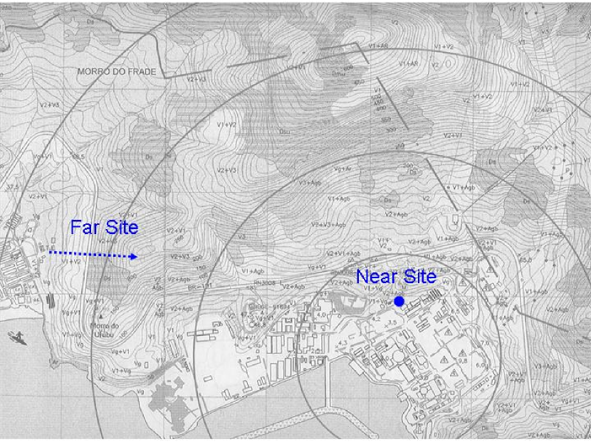
Figure 41: A topographic map of the nuclear reactor site at Angra dos Reis. The concentric circles are at 500 meter radial intervals from the core of Angra-II. Proposed locations for the near and far detector experimental halls as well as the far detector access tunnel are shown.

A topographic map of the site is shown in Figure 41. The concentric circles are at 500 m radial intervals from the primary Angra-II reactor core. The near site location is 300-350 m from the core. It has the possibility to gain about 15-20 m of rock overburden (30-50 meters of water equivalent). The far site location would exist under a 240 m hill at about 1350 m from the reactor core. Access to the far site would come from a 420 m tunnel which starts from the western edge of the hillside. This location is easily accessible from the town of Praia Brava and would be very near to the current location of their sewage treatment plant.

It is envisaged to place identical 50ton fiducial detectors at each location. Exact detector designs have not yet been developed, but it is currently assumed that such detectors would build off of the developments from other groups. Most likely a 3 volume detector would be optimal: a central liquid scintillator volume that would be doped with gadolinium (target); a surrounding volume of liquid scintillator without gadolinium (gamma catcher); a non-scintillating buffer to shield the radioactivity of the photo-tubes which would be installed at the outer edge of this volume. An active muon shield would then be required to surround this system. A spherical detector with an active target of 50 tons would have a total diameter of approximately 7.3 meters. The access tunnels and experimental halls are being designed to accommodate these dimensions.

A.4 Experimental Reach

Preliminary estimations have been performed of the signal and background rates for the given detector configuration. The detector at the far location is expected to get about 120 signal events per day, while the near site would be expected to receive about 3000. Some very preliminary background estimates suggest that at the far detector, less than 10 Hz uncorrelated backgrounds, which would easily be vetoed by an active muon shield, would be expected and there would be about 1-2 correlated background events per day from muon induced radioactive isotopes. Similarly at the near detector there would be an uncorrelated background rate of about 830 Hz (yielding an active live time of 63% after muon vetoing) and a correlated background of approximately 150 events per day. Having a signal to noise rate of about 100 in the far detector and 20 in the near detector should allow reasonable background rejection while maintaining statistical sensitivity. Figure 42 shows the expected statistical sensitivity as a function of time, for the best fit value and 90% allowed limits of $\Delta m^{2}$ from Super-Kamiokande. As can be seen, a limit of $sin^{2}(2\theta_{13})<0.02$ at 90% confidence level can be achieved within 3 years. Also in Figure 42 is shown the complete limit and 3$\sigma$ discovery potential for a 3 year run over all $sin^{2}(2\theta_{13})$ and $\Delta m^{2}$.

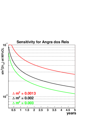
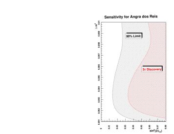
Figure 42: Expected sensitivity to $\sin^{2}(2\theta_{13})$ which could be achieved by an experiment at Angra dos Reis assuming a 1% systematic error. The plot on the left shows the sensitivity as a function of years of running for three different values of $\Delta m^{2}$. On the right, the full coverage of $\Delta m^{2}$ vs. $\sin^{2}(2\theta_{13})$ is shown assuming three years of data taking. Curves for both the limit at 90% confidence level and the discovery at 3 $\sigma$ are shown. The current limit at 90% confidence is $\sin^{2}(2\theta_{13})<0.2$.

A.5 Brazilian Community and Support

The Brazilian community has recently been having in-depth discussions about this possibility. There exists significant theoretical and phenomenological support for neutrino oscillation work in Brazil already, primarily located in the Universidade Estadual de Campinas (UNICAMP) and the Universidade do São Paulo. The director of the Centro Brasileiro de Pesquisas F sicas (CBPF) in Rio de Janeiro has shown great enthusiasm for this project and has offered to make his institution the host of such an experiment. There exist strong experimental particle physics groups based mainly in Rio de Janeiro and São Paulo. They are already strongly involved with the Pierre Auger project as well as experiments based at Fermilab and CERN. They have expressed great interest in pursuing a project that is local to Brazil and several of the experimental members have already started working on producing a more realistic set of cost estimates and site plans.

While it’s not possible to put any real faith behind the numbers, some preliminary estimates have concluded that with the cheaper labor costs in Brazil, the civil construction could probably be achieved for 5-7 million dollars (US). The local Brazilian community is currently in consultation with the government to get a commitment to this project and for covering the complete costs of civil construction. For the detectors, a very conservative cost estimate concluded that they would require about 7 million dollars each. Thus the total project could probably be completed with an external contribution of less than 15 million dollars (US).

Appendix B The Double Chooz Project

Since the end of the year of 2002 a group of European (French, German, and Russian) physicists has been working on the possibility to measure the last undetermined neutrino mixing angle $\theta_{13}$ with a two detector reactor neutrino experiment. During the year 2003, a site investigation has been performed, and three sites have been selected to be potentially suitable to performed such a project: the Penly site (Normandie, France), the Cruas site (Ardèche, France), and the Chooz site (Ardennes, France). Thanks to its existing infrastructure and to the support of the EDF (Electricité De France) power plant staff, Chooz is the most reliable location to perform an experiment and we’ll only focus on it in the following.

B.1 The Double-CHOOZ concept

The new Chooz project will run two identical detectors of medium size, containing 10 to 20 tons of liquid scintillator target. The (still existing) neutrino laboratory of the first Chooz experiment, located at 1.05 km from the two cores of the Chooz powerful nuclear plant (PWR, 8.4 thermal GW) will be used again. We label this detector the far detector or CHOOZ-far. The CHOOZ-far site is shielded by about 300 mwe of $2.8\,g/cm^{3}$ rocks. We plan to start to take data at CHOOZ-far within the first month of the year 2007.

In order to cancel the systematic errors originating from the nuclear reactor (electron anti-neutrino flux and spectrum), as well as to reduce the set of systematic errors related to the detector and to the event selection procedure, a second detector will be installed close to the nuclear cores, within a range from 100 to 200 meters. We label this detector the near detector or CHOOZ-near. Since no natural hills or underground cavity exists at this location, an artificial overburden of a few tens of meter height has to be built. From the first discussions, this construction has been allowed by the power plant company authorities. A pre-study of the civil engineering work to be done for CHOOZ-near has been order and will be performed during the end of 2003. This pre-study which aims to determine the best combination location-overburden as well as to optimize the cost is financed by the French electricity power company EDF.

From the simulation, a new experiment at CHOOZ would reach a sensitivity of $\sin^{2}(2\theta_{13})\,<\,0.03$, at $90\%$ CL for $\Delta m^{2}_{atm}\,=\,2.0\times 10^{-3}\,\,eV^{2}$ (latest best fit value of the Super-Kamiokande experiment), after three years of operation. A sensitivity of $0.05$ would be reached within the first year of running with two detectors, improving the CHOOZ bound by roughly a factor of five. These estimates are based on the assumptions that the relative normalization error between the near and far detectors could be kept at $0.8\,\%$, and that the backgrounds at both sites amount to less than $1\,\%$ of the anti-neutrino signals.

It is worth mentioning that the 1.05 km average baseline at CHOOZ is not optimal (a little too short) compared to the first oscillation maximum (for anti-neutrino energy of a few MeV) if the atmospheric mass splitting would remain at $\Delta m^{2}_{atm}\,=\,2.0\times 10^{-3}\,\,eV^{2}$. A shorter baseline is compensated by higher statistics for a fixed size detector, however. A value of $\Delta m^{2}_{atm}\,<\,1.5\times 10^{-3}\,\,eV^{2}$, close to the $90\,\%$ CL current lower bound, would restrict the absolute potential of the double-CHOOZ experiment.

B.2 Detector design

The detector design foreseen is an evolution of the detector of the first experiment, (CHOOZ-I). The first improvement with respect to the CHOOZ-I sensitivity comes from an increase of the exposure to get more than 40,000 anti-neutrino events at CHOOZ-far. This condition translates to a statistical error lower than $0.5\,\%$. This increase of signal is obtained by using a target cylinder of 120 cm radius and 280 cm height, providing a volume of $14\,m^{3}$, 2.5 higher than in CHOOZ-I. In addition, the operation period will be extended to at least three years, and the efficiency will be improved (the global load factor of the reactor is about $80\,\%$ while it was much lower for the CHOOZ-I experiment due to the power plant commissioning). In addition, the background level will be decreased in order to get a signal to noise ratio greater than 100 (about 30 in CHOOZ-I).

The near and far detectors will be identical up to the PMTs surface. This will allow to have a relative normalization error less than $0.8\,\%$. However the outer shielding will not be identical since the cosmic background varies between CHOOZ-near and CHOOZ-far, due to the different overburdens. The overburden of the near detector has been chosen in order to keep the signal to background ratio above 100; with this condition, even a poor measurement of the background keeps the associated systematics error well below $1\,\%$.

The detector design was intensively studied and tested by Monte-Carlo simulation, using a code derived from the simulation of the CHOOZ-I experiment. The one meter low radioactive sand shielding of CHOOZ-I, used to reduce the external radioactivity contamination, will be replaced by a 15 cm stainless steel shielding. The size of the liquid active buffer can then be increased. From the center there will be:

• a 120 cm radius 280 cm height acrylic target cylinder, filled with $0.1\,\%$ Gd loaded liquid scintillator

• a 40 cm buffer of non-loaded liquid scintillator with the same optical properties (light yield, attenuation length), to get the full positron energy as well as most of the neutron energy released after the neutron capture (this buffer is called the $\gamma$ catcher)

• a 95 cm buffer of non scintillating liquid, to decrease the level of the accidental background

• a 60 cm veto filled with liquid scintillator.

The spatial reconstruction is not affected by the cylindrical shape. Each parameter of the detector is being studied by Monte-Carlo simulation, to define the tolerance on the differences between the two detectors. The inner volume dimensions as well as the shape of the target vessels are still preliminary and could change prior to the completion of the proposal. The aim is to reduce the number of analysis cuts with respect to the CHOOZ-I experiment to push down the systematic errors related to the anti-neutrino event selection in both detectors independently. The non-scintillating buffer will reduce the singles rates in each detector by two orders of magnitude with respect to CHOOZ-I. This lowers the positron threshold down to 500 keV, well below the 1 MeV physical threshold of the inverse beta decay reaction. A very low threshold has three advantages: a) the systematic error due to this threshold is then suppressed, b) the background below the threshold can be measured, c) the beginning of the positron spectrum provides an additional calibration point between the near and far detectors. This reduction allows the relaxation or even suppression of the localization cuts, such as the distance of an event to the PMT surface and the distance between the positron and the neutron. These cuts, used in CHOOZ-I, are difficult to calibrate and have to be avoided in a precision experiment. The remaining event selection cuts will have to be calibrated between the two detectors with a very high precision. The main cut to calibrate is the energy selection of the delayed neutron after its capture on a Gd nucleus (with a mean energy release of 8 MeV gammas). The requirement is 50-100 keV on the precision of this cut between both detectors, which is feasible with standard techniques using radioactive sources at different positions and lasers. The main sensitivity of a reactor experiment of the Double-CHOOZ scale (400 GW t y) is the total number of events; the requirements on the positron energy scale are then less stringent since the weight of the spectrum distortion is low in the analysis. This is being studied by simulation.

B.3 Backgrounds

The correlated background was measured in CHOOZ-I, and found to be about one event per day. At CHOOZ-far the active buffer will be increased by a factor of two, with a solid angle for the out-coming background being unchanged. This together with a signal increased by a factor of 2.5 will fulfill the requirement of a signal to noise ratio greater than 100.

At CHOOZ-near, due to the shallow depth, the cosmic background will be important. For a detector located at 150 meters from the cores, with an overburden of 55-65 mwe, the signal will be 5,000 events per day, while the muon rate is expected to be a factor of ten less. A dead time of 500 $\mu s$ will be applied after each muon, leading to a global dead time of about $25\,\%$. About 20 recoil proton events per day, mimicking the anti-neutrino signal, are expected while the estimate of the muon induced cosmogenic events (${}^{9}Li$ and ${}^{8}He$) is 15 per day with a large uncertainty (this last point is being studied). This fulfills the requirement of a signal to noise ratio greater than 100 at CHOOZ-near.

B.4 Conclusion and outlook

A new reactor neutrino experiment at the Chooz nuclear power plant has the potential to reach a sensitivity of $\sin^{2}(2\theta_{13})\,<\,0.03$, at $90\%\,$ CL for $\Delta m^{2}_{atm}\,=\,2.0\times 10^{-3}\,\,eV^{2}$, after three years of operation. This potential is similar to what could be achieved by future long baseline neutrino experiments (JPARC and NuMI-Off axis) at the horizon 2013. Furthermore, both results are complementary.

The CHOOZ-far detector will be installed in the fall of 2006, in order to start data taking in the beginning of 2007. Due to civil engineering constraints, the CHOOZ-near detector will be installed one year after CHOOZ-far, and will start data taking beginning 2008. The Double-CHOOZ proposal will be written in the forthcoming months by a team of European physicists from three countries and five laboratories (about 20 physicists); the international collaboration is expected to grow during this period.

We would like to thank the Electricité de France power company for its technical and financial support to the Double-CHOOZ project.

Appendix C Daya Bay

The Daya Bay nuclear power plant is the largest nuclear power generating station in China, and the tenth largest in the world. It consists of two twin reactor cores, one is called Daya as shown in Figure 43, and the other is called Lingao as shown in Figure 44, each core can generate a thermal power of 2.9 GW, making a total of 11.6 GW. All reactors are the type of the pressurized water. A third twin-core with a total thermal power of 5.8 GW, is planed to be online at about 2010. It will then be the second largest nuclear power plant in the world, only next to the Kashiwazaki in Japan.

Daya Bay is located about 50 km from ShenZhen, Guangdong province, and it is only two hours drive from Hong Kong. The reactors are build on coast next to a mountain whose highest point is 700 m above the sea level. A group of Chinese physicist has inspected the site and it seems no problem to have a near experimental hall with an overburden of 400 mwe at a distance of about 300 m to the core, and a far experimental hall with an overburden of 1200 mwe at a distance of about 1500-2000 m to the core. Initial discussions about the possible experiment with the authority of the power plant are positive and a conceptual design of the tunneling and experimental hall in collaboration with the power plant is underway.

A group of physicists has been working on the this possibility, including negotiation with the power plant, conceptual design of the experimental hall and tunneling, detector design and R&D, Monte Carlo simulation etc.,. Collaboration with all interested parts are welcome.

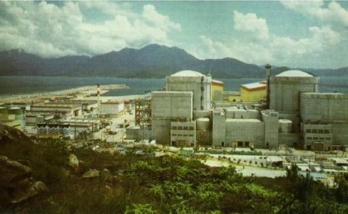
Figure 43: The overview of the Daya Bay nuclear power reactors

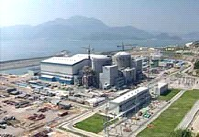
Figure 44: The overview of the Lingao nuclear power reactors

Appendix D The Diablo Canyon Power Plant

A number of commercial nuclear power plants worldwide are currently under evaluation as sites for a next-generation reactor neutrino oscillation experiment. An overview of these activities is given in this paper and references herein. One of the candidate sites in the United States is the Diablo Canyon Power Plant (DCPP) on the Central Coast in California. The Diablo Canyon Power Plant is located in San Luis Obispo County north of Santa Barbara and provides electricity to northern and central California. DCPP is owned by Pacific Gas and Electric Company (PG&E) [143].

A powerful reactor and overburden in excess of 300 mwe to shield the antineutrino detectors from cosmic rays and associated backgrounds are principal features of a suitable site for a reactor neutrino experiment. An underground detector facility or artificial overburden are usually required to achieve sufficient shielding from cosmic rays.

The Diablo Canyon Power Plant consists of two 1.1 MW reactor cores separated by $\sim 100$ m with a total thermal energy of 6.2 GW_th. Nearby coastal mountains provide the opportunity for good overburden and make the plant an almost ideal site for a reactor neutrino experiment [144]. The excavation of a horizontal tunnel in the coastal mountains can provide overburden of up to 800 mwe with distances up to $\sim 3$ km. The general layout and topography of the site allows the construction of a 1-2 km-long tunnel for two or more movable detectors. A picture of the Diablo Canyon Power Plant is shown in Figure  45 and Figure  46 gives a topographic map of the area surrounding the DCPP site.

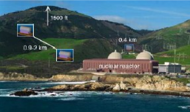
Figure 45: Picture of the Diablo Canyon nuclear power plant in San Luis Obispo County, California, USA. The local topography at Diablo Canyon allows the construction of an underground tunnel between 0.9-2 km for the placement of two or more neutrino detectors. A longer tunnel up to a distance of 3 km is possible. It may be possible to place an additional near detector at 0.4 km under artificial overburden.

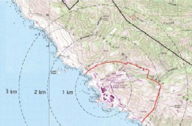
Figure 46: Topographic map of the site of the Diablo Canyon Power Plant. The land boundary (black) as well as the power plant site boundary (red) are indicated.

Construction of a horizontal tunnel is required to place the neutrino detectors underground and shield them from cosmic rays and associated backgrounds. The local topography allows the construction of a tunnel at distances between 0.9-2 km from the reactor. Longer tunnels up to a distance of 3 km are possible. A near detector within 500 m of the reactor cores requires the construction of a detector room and artificial overburden in excess of at least 50 mwe.

The neutrino detectors can be placed in detector rooms located in side drifts off the main tunnel (see Figure 47). This allows the detectors to be surrounded by a hermetic muon veto and passive shielding reducing the cosmic-ray induced neutron and external $\gamma$-background from the rock. The side drifts can provide a clean-room environment for the sensitive neutrino detectors and air control for the reduction of radon. Each side drift will have enough space to accommodate two neutrino detectors in order to allow for the relative calibration of the detectors’ efficiencies at one particular distance from the reactor and under the same background conditions. Due to the natural topography of the site the overburden and hence the cosmic ray background will vary depending on the detector location and the distance from the reactor.

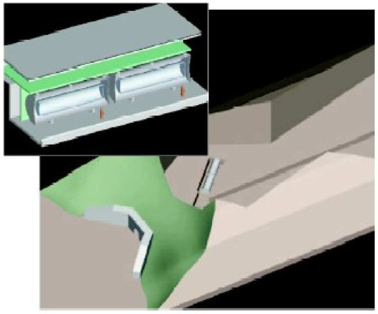
Figure 47: Horizontal access tunnel and side drifts for the the detector rooms. The side drifts will accommodate two neutrino detectors. (Drawings provided by D. Oshatz, LBNL.)

A horizontal access tunnel will allow for the possibility to optimize the baseline of the detectors with respect to the reactor. The exact location of the side drifts can be chosen when the parameters that determine the neutrino oscillation length (such as $\Delta m^{2}_{atm}$) and hence the baseline of the experiment are better known. With multiple side drifts for the detectors one can imagine demonstrating conclusively the subdominant oscillation effect with measurements at various locations along the tunnel.

Extensive geological studies of the site of the Diablo Canyon Power Plant have been done by PG&E. A preliminary evaluation of the geology for this project is in progress at Berkeley Lab. The geology of the site appears to be suitable for tunneling and the excavation of the underground detector rooms. A tunnel may even offer the opportunity for interesting geo-science studies. The stratigraphy of the Diablo Canyon region is dominated by three Pliocene-Miocene marine sedimentary units: the Pismo Formation, the Monterey Formation and the Obispo Formation. The rocks present in the area around the prospective tunnel sites at Diablo Canyon are predominantly the older sedimentary and volcanic rocks of the Obispo Formation, consisting of (1) tuffaceous siltstones and claystones, and (2) basaltic flows, dikes, and sills. There are a variety of geologic hazards and issues associated with the construction and maintenance of a neutrino detector facility at Diablo Canyon: landslide hazards, rock quality issues, seismic hazards, and water quality. These issues are currently under investigation. The average bulk density of these rock formations varies between 2.2-2.8 g/cm³. This leads to a maximum effective overburden of $\sim 800$ mwe at various locations along the tunnel. Geologic cross-sections of four possible tunnels at the DCPP site are shown in Figure 48. These tunnel cross-sections start at an elevation of $\sim 85$ m at a location approximately 0.9 km East-North-East from the Diablo Canyon Power Plant.

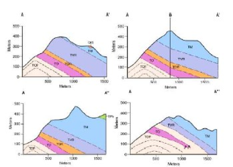
Figure 48: Geologic cross-sections of four possible tunnels at the DCPP site. The distance is given in meters from the tunnel portal. The tunnel portal is located at a distance of about 0.9 km from the reactor. A maximum overburden of up to 300 m of rock or $\sim 800$ mwe can be obtained. (Figure provided by C. Onishi and P. Dobson, LBNL.)

The physics potential of a next-generation reactor neutrino measurement is discussed in great detail in the previous sections of this paper. The ultimate sensitivity of such an experiment will strongly depend on the layout of the experiment including the distances from the reactor cores, the overburden, the size of the detectors, and our understanding of the relative detector response. The Diablo Canyon Power Plant is a site that offers the opportunity to design an experiment that meets these criteria and achieves an ultimate sensitivity of $\sin^{2}(2\theta_{13})=$ 0.01-0.02.

Appendix E An Illinois Reactor Experiment

The Illinois proposal is to locate the experiment at one of the Exelon nuclear reactors: Braidwood, Byron, or La Salle. All three of these reactors are located in northern Illinois with 100 km of both Argonne National Lab and Fermilab. The typical elevation of northern Illinois is about 250 meters and the topology is flat. The baseline experiment design calls for three identical spherical detectors, each with a 25 ton gadolinium loaded scintillating target. There is one near detector located at a distance of about 200 meters from the reactor cores. The remaining two detectors are at a far location and share a baseline of 1400 to 1800 meters. Both the near and the far detector halls are located below $\geq 100$ meters of rock ($\sim 300$ mwe). This shielding is achieved by digging shafts straight down to a depth of about 100 meters

In addition to the standard source and flasher calibration systems, the relative efficiency of the near and far detectors is measured head-to-head. To facilitate this measurement, the detectors are movable, and the near and far detector sites are connected by a tunnel (See Figure 25). The relative efficiency is measured with the two detectors side by side in the intense neutrino flux at the near detector site. Calibration running for 10% of the experimental run results in an uncertainty on the relative efficiency that is smaller than the statistical error on the event rate in the far detector.

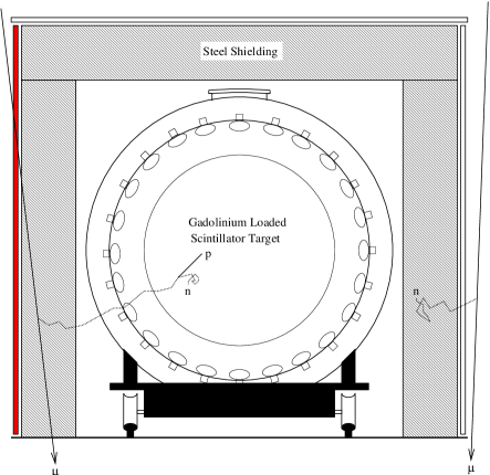
Figure 49: Interaction of the Muon Veto Neutron Shield system with muon induced fast neutrons produced both inside and outside the shielding bunker.

Correlated coincident backgrounds, in which both parts of the event are generated by the same initial interaction, are the most difficult to account for. Most correlated backgrounds are due to fast neutrons generated in cosmic ray $\mu$ spallation in the materials surrounding the detector. Inside the detector a fast neutron can strike a hydrogen nucleus giving it enough energy to mimic the positron. Alternatively, a neutron-carbon inelastic collision may result in the production of gamma rays. In both cases the fast neutron will thermalize and capture with nearly the same spatial and time correlation as the neutrons from inverse $\beta$-decay.

To deal with these correlated background events a Muon Veto Neutron Shield (MVNS) system is proposed. In the MVNS system (shown in Figure 49), the detector is housed in a bunker of dense material intended to range out neutrons. The outside of this bunker is covered in an array of plastic scintillator. The scintillator array detects muons entering the bunker. Muons in the bunker material may kick out fast neutrons and cause a correlated background event in the detector. If a muon passes close to the bunker without passing through, neutrons generated by it in the surrounding rock are ranged out by the bunker. In addition, matching the energy distribution for muon events to the neutrino candidate events, outside the reactor energy range, the any surviving background events can be subtracted from the neutrino event sample.

The MVNS bunker is fixed and does not move with the detector.

The Illinois proposal is designed to control the dominant systematic errors, which are due to the relative efficiency of the near and far detectors and the uncertainty in the background rate. By keeping these systematic errors low, a sensitivity of $\sin^{2}2\theta_{13}<0.01$ at 90% CL can be achieved in a three year run.

Appendix F The KASKA project

In the KASKA experiment [145], three identical detectors are to be built in the site of Kashiwazaki-Kariwa NPP which has 7 reactors, producing total thermal energy of 24.3 GW. This is the most powerful NPP in the world. Using a large-power nuclear power plant is profitable for obtaining not only a high event rate but also a low background-to-signal ratio at a given depth underground. The relative locations of reactors and detectors are shown in the fig.-50. Although the far/near distance ratios between the reactors and detectors are not unique, the effective uncertainty introduced from the variations of the distances are estimated to be only 0.2%.

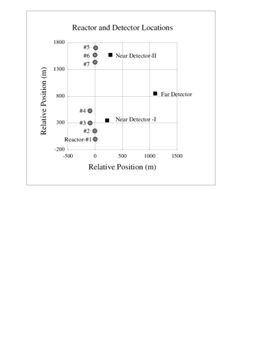
Figure 50: Reactor (circles) and detector (squares) relative locations. Reactor #1 through #4 form a cluster and #5 through #7 form another cluster. The two clusters separate about 1.3 km apart. Two near detectors will be placed at around 400 m from each cluster. The far detector will be placed at around 1.3 km from all the reactors.

The detector is a CHOOZ like detector as shown in the Figure 51.

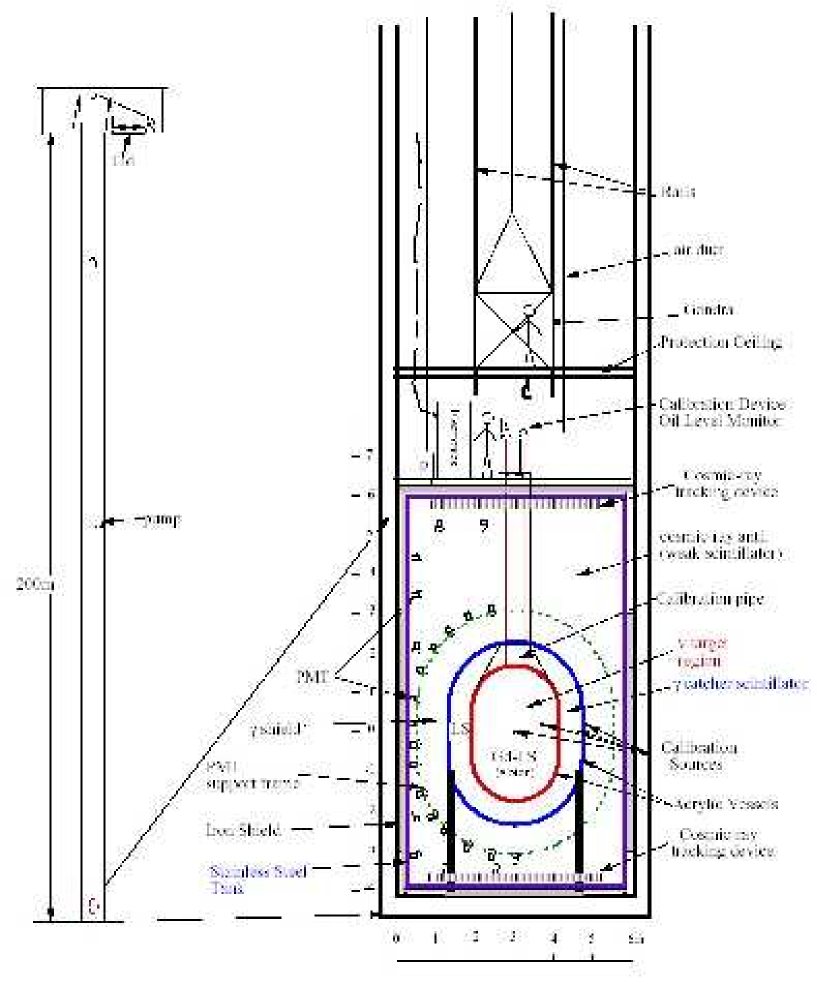
Figure 51: Schematic view of the detector.

The $\bar{\nu}_{e}$ target is 8 tons of Gadolinium loaded liquid scintillator (GD-LS) contained in a acrylic vessel which is called region-I. The component of the Gd-LS is the Palo Verde type, which is proven to be stable in the acrylic container [75].

The Gd concentration is 0.1% (0.15% optional) and the neutron capture efficiency on Gd is 88%. The optional 0.15% Gd concentration is intended to increase the neutron capture efficiency and to reduce the systematic uncertainties associating with the inefficiency. The reactor $\bar{\nu}_{e}$ is detected by the inverse $\beta$ decay reaction with proton.

$$\bar{\nu}_{e}+p\rightarrow e^{+}+n$$ (29)

The kinetic energy of the positron is neutrino energy minus 1.8 MeV. The positron annihilates with electron after slowing down in the LS and then produces two 0.511 MeV $\gamma$’s. This process produces a prompt signal, whose energy is between 1 MeV and 8 MeV.

The energy threshold for prompt signal is set to be below the minimum prompt signal energy of 1 MeV. In this way, no systematic ambiguities associated with threshold energy cut is introduced.

The neutron produced in the inverse $\beta$ decay reaction thermalizes quickly and is absorbed by Gd, producing $\gamma$-rays whose total energy amounts to 8 MeV. The neutron absorption signal occurs typically 30 $\mu s$ after the prompt signal.

The neutrino signal is defined by the existence of correlated signals. That is, when 8 MeV of energy deposit is observed after associating prompt signal whose energy is between 1 MeV and 8 MeV, this event is considered to be $\bar{\nu}_{e}$ event, regardless the positions of the signals. Because there is no position cut, the measured neutrino rate is free from the position reconstruction error. Requirements for the timing correlation between the positron signal and the neutron signal suppress backgrounds severely.

The main source of systematic error comes from the relative difference of the LS mass in the three detectors. The total volume of the LS will be controlled not by the size of the container but by the liquid volume put in the container. The relative volume of the introduced LS will be calibrated before putting in each detector. The total volume of the LS in the oval part of the vessel can be measured precisely from the total volume of introduced LS and the liquid level in the thin calibration pipe even if there is a distortion of the vessel after the installation. The relative uncertainty of the LS mass between detectors will be less than 0.5%.

If neutrino events occur near the boundary of region-I, $\gamma$ rays from the positron annihilation and the neutron absorption may escape from region-I. In such cases, the visible energies of the signals may become less than thresholds and this inefficiency introduces potential systematic error. This is also true for the case of positron detection.

In order to catch such $\gamma$ rays, a 50 cm thick Gd unloaded LS (region-II) surrounds region-I acrylic container. The light output of region-II LS is adjusted to be same as region-I LS to obtain accurate original energies accurately. It is estimated that most of the $\gamma$ rays can be contained within regions I and II and the inefficiencies of the positron and neutron signal is less than a few percent and the systematic error associated with this inefficiency is a fraction of a percent.

If the neutrino event occurs near the acyclic wall, the neutron may escape from region-I (spill-out effect). This kind of events produces a loss of efficiency. However, the inefficiency due to the spill-out effect is estimated to be only $\sim$3% and the systematic error due to the spill-out effect is estimated to be on the order of 0.1%. On the other hand, there is the opposite case that the inverse $\beta$ decay event occurs in region-II and then the resulting neutron spills into region-I (spill-in effect) and absorbed by Gd. This event is also considered to be a neutrino event and it amounts to 20% of the total events. However, the spill-in efficiency is insensitive to the hydrogen concentration in region-II LS because the spill-in event rate is proportional to the neutrino event rate and the neutron absorption length and both parameters have opposite dependence on the hydrogen concentration. Because most of the events are contained in regions I and II, systematic error due to the spill-in effect is estimated to be less than 0.5%.

The outer wall of region -II is also a acrylic container and the region-II is surrounded by a 90 cm thick scintillator with very slight light output (region-III). Region-III shields $\gamma$-rays from PMT glasses. Thanks to the region-III buffer, the singles rate is expected to become less than 10 Hz.

The outer most layer (Region-IV) is muon anti-counter filled with the same scintillator as region-III. These layers work as a shield of gamma rays and as cosmic ray anti counters. The slight light output is to detect low energy muons whose velocity is below the Cerenkov threshold, and to obtain high muon tagging efficiency. There will be about 400 8-inch low background PMTs at the boarder of region-III and IV. The wall between region-III and IV is just for light shield and no hermeticity is necessary.

There are cosmic-ray tracking devices on both the top and bottom of region-IV. The trackers are used to measure cosmic-ray tracks with accuracy of $\sim$10 cm. The cosmic-ray spallation background rate, such as the ⁹Li rate, is estimated from the excess at small distances in the distribution of distance between the neutrino event candidates and the cosmic-ray tracks. In order to stop the hadronic and soft part of the direct cosmic rays, the thickness of the top part of region-IV will be made thick. Region-IV LS is contained in a stainless steel cylindrical hermetic container. Outside the stainless steel container, there is a thick iron shield to prevent $\gamma$-rays coming from the soil outside.

The far detector will be placed at the bottom of a 200 m shaft hole with an inner diameter of 6 m. The cosmic-ray flux at the bottom is about 0.35 $m^{-2}s^{-1}$. Although there is open space above the detector, the cosmic-ray rate directly down the open space is only a fraction of that which reaches the detector penetrating the soil. The near detectors will be placed at the bottom of a 70 m depth shaft hole. This depth is chosen to make muon/neutrino ratio approximately equal to or slightly larger than the far detector case.

The major component of the background comes from fast neutrons produced in nuclear interactions caused by cosmic rays going through the rock near by. The visible energy distribution of the prompt signal in the fast neutron backgrounds was measured to be flat by CHOOZ group at the energy range below 30 MeV [10] and this kind of background rate can be estimated by using the event rate within non-reactor-$\bar{\nu}_{e}$ energy range, such as below 1 MeV and above 10 MeV.

The absolute background rate is expected to be less than 2% and the error associated with estimation of the background will be less than 0.3%.

The systematic error in CHOOZ experiment was 1.7% (detector associated) $\oplus$ 2.1%(neutrino flux associated). The systematic error associated with the neutrino flux is reduced to 0.2% by comparing near and far detectors in the KASKA experiment. The systematic error associated with the detector is estimated to be between 0.5% and 1%. Because the neutrino oscillation at the near detectors is small, the consistency check of the systematic error estimation can be performed by comparing data of the two near detectors.

In two years of operation, 40,000 neutrino events will be recorded in the far detector and ten times more in the near detectors and the corresponding statistical error will be 0.5%. The 90% CL sensitivity of this experiment is shown in the fig.-52. At $\Delta m^{2}\sim 3\times 10^{-3}eV^{2}$, the sensitivity of $\sin^{2}2\theta_{13}\sim 0.02$ is expected. This is five times better limit than CHOOZ.

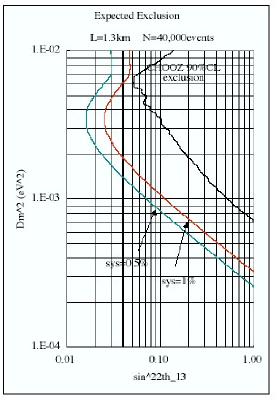
Figure 52: The expected 90%CL exclusion region of this experiment for the case of $\sigma_{sys}$=1% and 0.5% obtained by rate only analysis.

Appendix G The Krasnoyarsk Reactor and KR2DET

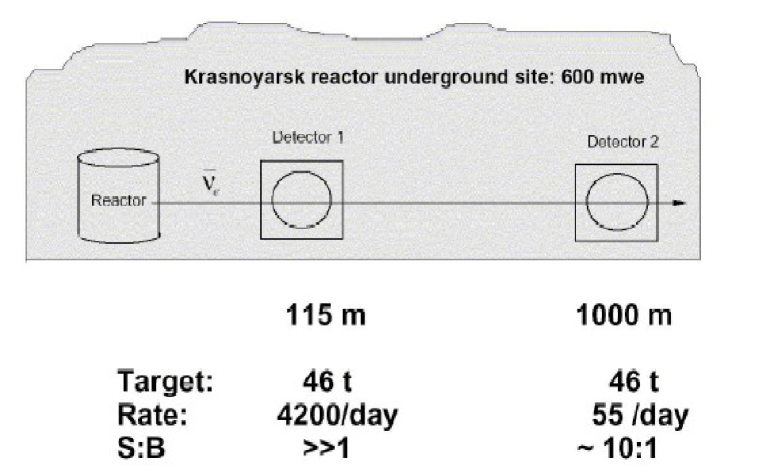
Figure 53: Scheme of the KR2DET experiment.

The KR2DET proposal is to place two identical liquid scintillation spectrometers are stationed at distances $L_{far}\approx$ 1000 m (far position) and $L_{near}\approx$ 115 m from the underground Krasnoyarsk reactor. (Figure 53) The overburden at Krasnoyarsk is $\sim$ 600 m.w.e., which is twice as much as in the CHOOZ experiment. (At short distances form the reactor the one reactor - 2 detector approach was first probed at Rovno [146] and later successfully used at Bugey [147].

Two types of analysis can be used. Analysis I is based on comparison of the shapes of positron spectra $S(E_{e})_{far}$ and $S(E_{e})_{near}$ measured simultaneously in two detectors. In no oscillation case the ratio $S(E_{e})_{far}/S(E_{e})_{near}$ is energy independent. Small deviations from the constant value of this ratio

$$X_{shape}=C\cdot\frac{1-\sin^{2}2{\theta}\cdot\sin^{2}\left(\frac{1.27{\Delta}m^{2}L_{far}}{E}\right)}{1-\sin^{2}2{\theta}\cdot\sin^{2}\left(\frac{1.27{\Delta}m^{2}L_{near}}{E}\right)}$$ (30)

are searched for oscillation parameters.

In the one reactor - two detector scheme

• Results of the Analysis I do not depend on the exact knowledge of the reactor power, absolute $\bar{{\nu}_{e}}$ flux and energy spectrum, burn up effects, absolute values of hydrogen atom concentrations, detection efficiencies, target volumes and reactor - detector distances.

• At Krasnoyarsk the detector backgrounds can be measured during reactor OFF periods, which periodically follow 50 day long reactor ON periods.

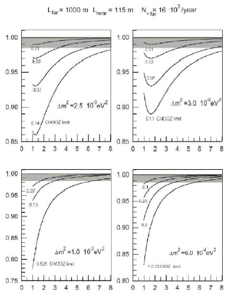
Figure 54: Calculated ratio of positron spectra $S(E_{e})_{far}/S(E_{e})_{near}$ for some oscillation parameters. Values of $\sin^{2}(2\theta)$ are shown at the curves.

Calculated ratios $S(E_{e})_{far}/S(E_{e})_{near}$ for a set of oscillation parameters are shown in Figure 54.

Analysis II is based on the ratio of the total number of neutrinos $N_{far},N_{far}$ detected at two distances:

$$X_{rate}(\sin^{2}2{\theta},{\Delta}m^{2})=\left(\frac{L_{far}}{L_{near}}\right)^{2}\cdot\left(\frac{V_{near}}{V_{far}}\right)\cdot\left(\frac{{\epsilon}_{near}}{{\epsilon}_{far}}\right)\cdot\left(\frac{N_{far}}{N_{near}}\right)$$ (31)

$V_{far},V_{near},{\epsilon}_{far},{\epsilon}_{near}$ are the target volumes and neutrino detection efficiencies. In no oscillation case $X_{rate}$ = 1.

Analysis II is also independent of the exact knowledge of the reactor neutrino flux and energy spectrum. The absolute values of detection efficiencies are practically canceled, only their small difference is to be considered here while the ratios $(L_{far}/L_{near})^{2}$ and $(V_{near}/V_{far})$ should be known accurately.

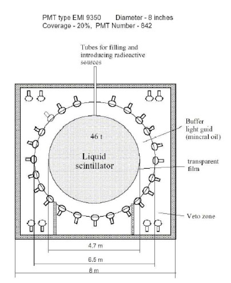
Figure 55: The KR2DET $\bar{\nu}_{e}$ spectrometer (schematic).

A miniature version of the KamLAND [148] and BOREXINO [149] and a scaled up version of the CHOOZ three - concentric zone detector design is chosen for the construction of the spectrometers (Figure 55). KR2DET plans a 4.7 m diameter liquid scintillator target, enclosed in transparent spherical balloon. The target is viewed by $\sim$800 8-inch EMI-9350 (9350 - 9356) photomultipliers trough $\sim$90 cm layer of mineral oil of the zone-2 of the detector. The PMTs of this type have successfully been used in the CHOOZ experiment and are used now in the BOREXINO and SNO detectors [150]. A 20% light collection and 150 - 200 photoelectron signal is expected for 1 MeV positron energy deposition. The PMTs are mounted on the stainless steel screen, which separates external zone-3 from the central zones of the detector. The $\sim$75 cm thick zone-3 is filled with mineral oil (or liquid scintillator) and serves as active (muon) and passive shielding from the external radioactivity.

The ratio of measured positron spectra $S(E_{e})_{far}/S(E_{e})_{near}$ in Equation (30) can be slightly distorted because of relative difference in response functions of the two “identical” spectrometers.

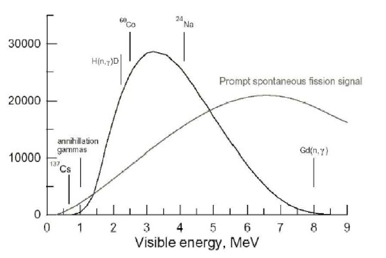
Figure 57: Positron visible energy spectrum.

The goal of calibration procedures is to measure this difference and introduce necessary corrections. This can be done by a combination of different methods. First there will be a periodic control of the energy scales in many points using ${\gamma}$-sources shown by arrows in Figure 57. A useful continuous monitoring of the scales at 2.23 MeV can provide neutrons produced by trough going muons and captured by the target protons during veto time.

The second method uses small spontaneous fission ²⁵²Cf or ²³⁸U sources periodically placed in the detectors. These sources generates continuous energy spectrum due to prompt fission gammas and neutron recoils (the dashed line in Figure 57.). Deviation from unity of the measured spectra can be used to calculate relevant corrections.

The goal is that the systematic uncertainty due to detector spectrometric difference essential for Analysis I can be controlled down to 0.5%.

In Analysis II the systematic uncertainty in the quantity $(L_{far}/L_{near})^{2}\cdot(V_{near}/V_{far})\cdot({\epsilon}_{near}/{\epsilon}_{far})$ in Equation (31) can hopefully be kept within 0.8%.

The choice of the scintillator has not been made so far. There should be progress in manufacturing Gd ($\sim$0.9 g/liter) loaded scintillators to improve the response to neutrons and suppress accidentals, which originate from U/Th gammas coming from surrounding rock. The Palo Verde Gd-scintillator showed better stability than the scintillator used in CHOOZ. The LENS project considers scintillators with rare earth contents as high as $\sim$50 g/liter. One possibility is scintillator without Gd based on the mixture of isoparaffin or mineral oil and pseudocumene ($\sim$20%) with $\sim$2g/liter PPO as primary flour. This scintillator has C/H ratio 1.85, density 0.85 kg/liter and $0.785\times 10^{29}$ H atoms per ton.

The neutrino events satisfy the following requirements: (i) a time window on the delay between $e^{+}$ and neutron signals 2$-$600 ${\mu}$s, (ii) energy window for the neutron candidate 1.7$-$3.1 MeV and for $e^{+}$ 1.2$-$8.0 MeV, (iii) distance between $e^{+}$ and neutron less than 100 cm. At this stage no pulse shape analysis to reject proton recoils is planned.

Under these assumptions neutrino detection efficiency of 75% was found and neutrino detection rate $N(e^{+},n)$ = 55/day calculated for the far detector.

The time correlated background 0.1 per day per one target ton was found by extrapolation of the value 0.25/per day per target ton measured at CHOOZ:

$${\rm CHOOZ\ (300\ mwe),\ 0.25/day}\cdot{\rm ton}\rightarrow{\rm Kr2DET\ (600\ mwe),\ 0.1/day}\cdot{\rm ton}$$ (32)

The accidental coincidences come from the internal radioactivity of detector materials and U and Th contained in the surrounding rock. The internal component of the background was estimated to be less 0.3/day, which is an order of magnitude smaller than the rate of the correlated background (see hep-ph/0109277). In contrast to the KamLAND and Borexino experiments three orders higher concentrations of U, Th, K and Rn can be tolerated in the liquids used in the Kr2DET case.

First estimations of accidentals coming from the radioactivity of the rock showed however that external passive shielding of the detector should be increased in case scintillator without Gd is used as the neutrino target.

Calculated neutrino detection rates $N(e^{+},n)$ and backgrounds for scintillator with no Gd are summarized in Table 16.

Table 16:

Detector	Distance,	Target,	$N(e^{+},n)$,	$N(e^{+},n)$,	Backgr., day-1
	m	mass, ton	day-1	year-1∗	correl.	accid.∗∗
Far	1000	46	55	$16.5\cdot 10^{3}$	5	$\sim$0.3
Near	115	46	4200	$12.5\cdot 10^{5}$	5	$\sim$0.3

^∗ 300 days/year at full power.
^∗∗ due to internal radioactivity of the detector materials only.

Expected 90% CL constraints on the oscillation parameters (Figure 56, curves K2Det) are obtained for 40000 detected $\bar{{\nu}_{e}}$ in the far detector (750 days of full power). The systematic uncertainties ${\sigma}_{shape}$= 0.5% in the Analysis I (“shape”) and ${\sigma}_{rate}$= 0.8% in the Analysis II (“rate”) have been assumed. The “shape” analysis is somewhat more sensitive and can shift (at ${\Delta}m^{2}=2.5\times 10^{-3}$ eV² the $\sin^{2}2{\theta}$ upper limit from 0.14 (CHOOZ) to 0.017.

The one reactor - two detector approach fully eliminates uncertainties associated with the reactor neutrino source inherent to the absolute method used at CHOOZ.

Small relative difference in conceptually identical detector properties can be minimized through calibration and monitoring procedures.

The detector backgrounds can be measured during reactor OFF periods, which periodically follow 50 day long reactor ON periods.

Good signal to background ratio can be achieved due to sufficiently deep underground position of the detectors.

High statistics can be accumulated in reasonably short time period using detectors with $\sim$45 ton targets, which are relatively small if compared to modern neutrino detectors.

Neutrino community has accumulated positive experience in building and running 3 concentric zone detectors similar to the Kr2DET detectors.

G.1 Krasnoyarsk site details

The reactor belongs to the Federal State-Owned Unitary Enterprise MINING & CHEMICAL COMBINE (MCC) 53, Lenin Str., Zhelezhnogorsk, Krasnoyarsk Territory, RUSSIA, 660972.

The Krasnoyarsk neutrino laboratory is built in the MCC underground territory.

There are two places to install the detectors. One of them at $\sim$115 m from the reactor is 10 m high $15\times 15$ m square room. The other is a 125 m long, 11.5 high and 15 m wide corridor at $\sim$1000 m from the reactor. More information on neutrino at Krasnoyarsk can soon be found at
http://www.lngs.infn.it/site/exppro/panagic/section$\_$indexes/frame$\_$particles.html
(click “Laboratories and experiments”, then “Underground and underwater laboratories” and go to “Krasnoyarsk neutrino laboratory”)

Zhelezhnogorsk is located at about 70km from Krasnoyarsk on the bank of the Yenisei River. Zhelezhnogorsk is a very nice and clean town built in direct neighborhood to the Siberian taiga, rich of birds and animals. There is a beautiful large lake in the center of the town. Picturesque hills surround the town center. A musicale theater, hotel, rest home, restaurants, a lot of shops are in Zhelezhnogorsk.. The weather is comfortable; the number of sunny days is the same as in resort Sochi (at the Black Sea). Winter is cold but not so much compared with Moscow, air is dry. The summer and autumn are warmer and sunnier than in Moscow.

Some information about tourism in Krasnoyarsk Territories is available at the site: $http://tlcom.krs.ru/kalinka/indexe.htm$,
tours $http://tlcom.krs.ru/kalinka/indexe.htm$

Every day there are flights from Moscow to Krasnoyarsk airport. Big comfortable airbus IL86 in 4.5 hours time brings you from Moscow to Krasnoyarsk with good service of KrasAir company and a special minivan in 2 hours carries you from Krasnoyarsk airport Yemelianovo directly to the center of Zhelezhnogorsk.

MINING & CHEMICAL COMBINE has two own rest homes; one of them is in the town territory near the forest and another outside of the town not far from it on the bank of Yenisei River. Both of them have conference halls, comfortable living rooms and dining rooms.

Figure 56: Reactor antineutrino oscillation plots. Curves “CHOOZ”, “KR2DET” (expected) “shape” and “rate” are 90% CL $\bar{\nu}_{e}$ disappearance limits. The KR2DET limits are obtained assuming 40,000 detected antineutrinos in the far detector, 10:1 effect to background ratio and systematic uncertainties $\sigma_{shape}$ = 0.5% and $\sigma_{rate}$ = 0.8%. The shaded area represents the most probable atmospheric neutrino mass parameter region.

References

- [1] M. Maltoni, T. Schwetz, M. A. Tortola, and J. W. F. Valle. Status of three-neutrino oscillations after the sno-salt data. 2003.
- [2] G.L. Fogli et al., Phys. Rev. D67, 073002 (2003), [hep-ph/0212127]; hep-ph/0308055.
- [3] Super-K Coll., Y. Fukuda et al., Phys. Rev. Lett. 81 (1998) 1562; Y. Hayato, talk at the HEP2003 conference (Aachen, Germany, 2003), http://eps2003.physik.rwth-aachen.de
- [4] M.H. Ahn et al., K2K Coll., Phys. Rev. Lett. 90, 041801 (2003), [hep-ex/0212007].
- [5] S. Fukuda et al., Phys. Lett. B 539 (2002) 179; B.T. Cleveland et al., Astrophys. J. 496, 505 (1998); D.N. Abdurashitov et al., Phys. Rev. C60, 055801 (1999); astro-ph/0204245; W. Hampel et al., Phys. Lett. B447, 127 (1999); C. Cattadori, Nucl. Phys. B (Proc. Suppl.) 110 (2002) 311; Q. R. Ahmad et al., SNO Coll., Phys. Rev. Lett. 89, 011301 (2002); Phys. Rev. Lett. 89, 011302 (2002).
- [6] SNO collaboration, preprint nucl-ex/0309004, submitted to Phys. Rev. Lett. 2003.
- [7] K. Eguchi et al., Phys. Rev. Lett. 90 021802 (2003).
- [8] A. Aguilar et al. Evidence for neutrino oscillations from the observation of anti-nu/e appearance in a anti-nu/mu beam. Phys. Rev., D64:112007, 2001.
- [9] G. C. Branco et al. Minimal scenarios for leptogenesis and cp violation. Phys. Rev., D67:073025, 2003.
- [10] M. Apollonio et al., Eur. Phys. J. C27 (2003) 331-374.
- [11] M. Apollonio et al. Limits on neutrino oscillations from the CHOOZ experiment. Phys. Lett., B466:415–430, 1999.
- [12] F. Boehm et al., Phys. Rev. Lett. 84, 3764 (2000).
- [13] M. Lindner. The physics potential of future long-baseline neutrino oscillation experiments. 2002.
- [14] M. Freund, P. Huber, and M. Lindner. Systematic exploration of the neutrino factory parameter space including errors and correlations. Nucl. Phys., B615:331–357, 2001.
- [15] K. Hagiwara et al. Review of particle physics. Phys. Rev., D66:010001, 2002.
- [16] ”The Science Ahead, The Way to Discovery” The High-Energy Physics Advisory Panel long range plan for U.S. high-energy physics in the 21st century. PDF version, (approved by HEPAP, January 28, 2002). Available at http://doe-hep.hep.net/hepapbook/hepapplan/HEPAP_LRP_web.pdf
- [17] “High-Energy Physics Facilities Recommended For The DOE Office of Science Twenty-Year Roadmap”, March 2003, available at http://doe-hep.hep.net/HEPFacSub/HEPAP_FacilitiesMar03.pdf
- [18] “Facilities for the Future of Science, A Twenty-Year Outlook”, presented by the DOE Office of Science, November 2003. Available at http://www.sc.doe.gov/Sub/Facilities_for_future/20-Year-Outlook-screen.pdf
- [19] P. Vogel and J. F. Beacom, Phys. Rev. D 60, 053003 (1999) [arXiv:hep-ph/9903554].
- [20] C. Bemporad et al., Rev.Mod.Phys. 74 (2002) 297.
- [21] H. Minakata, H. Sugiyama, O. Yasuda, K. Inoue, and F. Suekane. Reactor measurement of theta(13) and its complementarity to long-baseline experiments. Phys. Rev., D68:033017, 2003.
- [22] A. Cervera et al. Golden measurements at a neutrino factory. Nucl. Phys., B579:17–55, 2000.
- [23] Martin Freund. Analytic approximations for three neutrino oscillation parameters and probabilities in matter. Phys. Rev., D64:053003, 2001.
- [24] J. Burguet-Castell, M. B. Gavela, J. J. Gomez-Cadenas, P. Hernandez, and O. Mena. On the measurement of leptonic cp violation. Nucl. Phys., B608:301–318, 2001.
- [25] Hisakazu Minakata and Hiroshi Nunokawa. Exploring neutrino mixing with low energy superbeams. JHEP, 10:001, 2001.
- [26] Gian Luigi Fogli and E. Lisi. Tests of three-flavor mixing in long-baseline neutrino oscillation experiments. Phys. Rev., D54:3667–3670, 1996.
- [27] V. Barger, D. Marfatia, and K. Whisnant. Breaking eight-fold degeneracies in neutrino CP violation, mixing, and mass hierarchy. Phys. Rev., D65:073023, 2002.
- [28] Patrick Huber, Manfred Lindner, and Walter Winter. Superbeams versus neutrino factories. Nucl. Phys., B645:3–48, 2002.
- [29] Y. Itow et al. The JHF-Kamioka neutrino project. Nucl. Phys. Proc. Suppl., 111:146–151, 2001.
- [30] P. Huber, M. Lindner, T. Schwetz, and W. Winter. Reactor neutrino experiments compared to superbeams. Nucl. Phys., B665:487–519, 2003.
- [31] G. L. Fogli et al. Addendum to: Solar neutrino oscillation parameters after first KamLAND results. 2003.
- [32] P. Huber, M. Lindner, and W. Winter. Synergies between the first-generation JHF-SK and NuMI superbeam experiments. Nucl. Phys., B654:3–29, 2003.
- [33] In 2003, a reanalysis of Super-Kamiokande atmospheric data has been presented extensively at conferences, e.g. Lepton-Photon 2003, Fermilab Illinois. See Nishikawa, http://conferences.fnal.gov/lp2003/program/S10/nishikawa_s10.pdf
- [34] T. Yanagida, in Proceedings of the Workshop on the Unified Theory and the Baryon Number in the Universe (O. Sawada and A. Sugamoto, eds.), KEK, Tsukuba, Japan, 1979, p. 95; S. L. Glashow, The future of elementary particle physics, in Proceedings of the 1979 Cargèse Summer Institute on Quarks and Leptons (M. Lévy et al., eds.), Plenum Press, New York, 1980, pp. 687–713; M. Gell-Mann, P. Ramond, and R. Slansky, Complex spinors and unified theories, in Supergravity (P. van Nieuwenhuizen and D. Z. Freedman, eds.), North Holland, Amsterdam, 1979, p. 315; R. N. Mohapatra and G. Senjanović, Neutrino mass and spontaneous parity violation, Phys. Rev. Lett. 44 (1980), 912.
- [35] S. M. Barr and I. Dorsner, Nucl. Phys. B 585, 79 (2000) [arXiv:hep-ph/0003058].
- [36] Guido Altarelli and Ferruccio Feruglio. Theoretical models of neutrino masses and mixings. 2002.
- [37] R. Barbieri, T. Hambye and A. Romanino, JHEP 0303, 017 (2003) [arXiv:hep-ph/0302118].
- [38] M. C. Chen and K. T. Mahanthappa, arXiv:hep-ph/0305088.
- [39] Stefan Antusch, Joern Kersten, Manfred Lindner, and Michael Ratz. Running neutrino masses, mixings and CP phases: Analytical results and phenomenological consequences. 2003.
- [40] H. S. Goh, R. N. Mohapatra and S. P. Ng, hep-ph/0308197.
- [41] T. Asaka, W. Buchmuller and L. Covi, Phys. Lett. B 563, 209 (2003) [arXiv:hep-ph/0304142].
- [42] K. S. Babu, J. C. Pati and F. Wilczek, Nucl. Phys. B 566, 33 (2000) [arXiv:hep-ph/9812538].
- [43] T. Blazek, S. Raby and K. Tobe, Phys. Rev. D 62, 055001 (2000) [arXiv:hep-ph/9912482].
- [44] R. Kitano and Y. Mimura, Phys. Rev. D 63, 016008 (2001) [arXiv:hep-ph/0008269].
- [45] C. H. Albright and S. M. Barr, Phys. Rev. D 64, 073010 (2001) [arXiv:hep-ph/0104294].
- [46] N. Maekawa, Prog. Theor. Phys. 106, 401 (2001) [arXiv:hep-ph/0104200].
- [47] G. G. Ross and L. Velasco-Sevilla, Nucl. Phys. B 653, 3 (2003) [arXiv:hep-ph/0208218].
- [48] M. C. Chen and K. T. Mahanthappa, Phys. Rev. D 68, 017301 (2003) [arXiv:hep-ph/0212375].
- [49] S. Raby, Phys. Lett. B 561, 119 (2003) [arXiv:hep-ph/0302027].
- [50] W. Buchmuller and D. Wyler, Phys. Lett. B 521, 291 (2001) [arXiv:hep-ph/0108216].
- [51] M. Bando and M. Obara, Prog. Theor. Phys. 109, 995 (2003) [arXiv:hep-ph/0302034].
- [52] W. Grimus and L. Lavoura, JHEP 0107, 045 (2001) [arXiv:hep-ph/0105212].
- [53] W. Grimus and L. Lavoura, Phys. Lett. B 572, 189 (2003) [arXiv:hep-ph/0305046].
- [54] K. S. Babu, E. Ma and J. W. F. Valle, Phys. Lett. B 552, 207 (2003) [arXiv:hep-ph/0206292].
- [55] R. Kuchimanchi and R. N. Mohapatra, Phys. Lett. B 552, 198 (2003) [arXiv:hep-ph/0207373].
- [56] T. Ohlsson and G. Seidl, Nucl. Phys. B 643, 247 (2002) [arXiv:hep-ph/0206087].
- [57] S. F. King and G. G. Ross, Phys. Lett. B 574, 239 (2003) [arXiv:hep-ph/0307190].
- [58] M. Honda, S. Kaneko and M. Tanimoto, JHEP 0309, 028 (2003) [arXiv:hep-ph/0303227].
- [59] R. F. Lebed and D. R. Martin, arXiv:hep-ph/0312219.
- [60] M. Bando, S. Kaneko, M. Obara and M. Tanimoto, arXiv:hep-ph/0309310.
- [61] A. Ibarra and G. G. Ross, Phys. Lett. B 575, 279 (2003) [arXiv:hep-ph/0307051].
- [62] T. Appelquist and R. Shrock, Phys. Lett. B 548, 204 (2002) [arXiv:hep-ph/0204141].
- [63] T. Appelquist, M. Piai, and R. Shrock, Phys. Rev. D, in press [arXiv:hep-ph/0308061].
- [64] P. H. Frampton, S. L. Glashow and T. Yanagida, Phys. Lett. B 548, 119 (2002) [arXiv:hep-ph/0208157].
- [65] J.-w. Mei and Z.-z. Xing, arXiv:hep-ph/0312167.
- [66] Andre de Gouvea and Hitoshi Murayama. Statistical test of anarchy. 2003.
- [67] R. N. Mohapatra, M. K. Parida and G. Rajasekaran, arXiv:hep-ph/0301234.
- [68] Lawrence J. Hall, Hitoshi Murayama, and Neal Weiner. Neutrino mass anarchy. Phys. Rev. Lett., 84:2572–2575, 2000.
- [69] M. Appollonio et al., Phys. Lett. B 420, 397 (1998).
- [70] Y. Fukuda et al., Phys. Lett. B 335, 237 (1994).
- [71] R. Becker-Szendy et al., Phys. Rev. Lett. 69, 1010 (1992).
- [72] E. Peterson et al., Nucl. Phys. Proc. Suppl. 77, 111 (1999).
- [73] Y. Fukuda et al., Phys. Rev. Lett. 81, 1562 (1998).
- [74] F. Boehm et al., Phys. Rev. D 64 112001 (2001).
- [75] F. Boehm et al., , Phys. Rev. D 62, 072002 (2000).
- [76] F. Boehm et al., Phys. Rev. D 62, 092005 (2000).
- [77] A. G. Piepke, S. W. Moser and V. M. Novikov, Nucl. Instrum. Meth. A 432, 392 (1999).
- [78] G. Gratta et al., Nucl. Instrum. Meth. A 400, 456 (1997).
- [79] Y. F. Wang et al., Phys. Rev. D 62 013012 (2000).
- [80] G. J. Feldman and R. D. Cousins, Phys. Rev. D 57, 3873 (1998).
- [81] C.L. Cowan et al., Science 124, 103 (1956).
- [82] See the results of H. Kerret’s Monte Carlo presented at Workshop on Future Low-Energy Neutrino Experiments, Munich, October 9-11, 2003. In particular see slide 39 in http://www1.physik.tu-muenchen.de/lehrstuehle/T30d/events/reactor03/pages/transparencies/lasserre.pdf
- [83] Y. Kozlov et al., Nucl.Phys.Proc.Suppl. 87 (2000) 514-516.
- [84] H. Minakata et al., hep-ph/0211111.
- [85] Harry Wong, personal communication.
- [86] M. Goodman et al., “Physics Potential and Feasibility of UNO”, June 2001; C.K. Jung and C. McGrew, “UNO (Underground Nucleon decay and Neutrino Observatory)”, February 7, 2003 at http://ale.physics.sunysb.edu/uno/UNO_Narrative.pdf
- [87] P. Huber et al., Nucl.Phys. B665 (2003) 487-519
- [88] A. Piepke and B. Cook, Nucl. Intrum. Meth. A385 (1997) 85.
- [89] H.Kwon, et al., Phys.Rev.D 24, 1097 (1981).
- [90] G.Zacek, et al., Phys.Rev.D 34, 2621 (1986).
- [91] A.I.Afonin, et al., Sov.J.Nucl.Phys. 46, 944 (1987); talk given at Neutrino-90, Geneva, June 10-15 (1990).
- [92] G.S.Vidyakin, et al., JETP Lett. 59, 25 (1994).
- [93] M.Abbes, et al., NIM A 374, 164 (1996);
- [94] B.Achkar, et al., Nucl.Phys.B 434, 503 (1995).
- [95] Z.D.Greenwood, et al., Phys.Rev.D 53 6054 (1996).
- [96] Y.Fukuda, et al., Phys.Lett. 452 418 (1999).
- [97] derived from F.Ashton, H.J.Edwards, and G.N.Kelly, J.Phys.A 4 352 (1971).
- [98] J.C.Gosse and F.M.Phillips, Quaternary Science Reviews 20(14), 1475 (2001).
- [99] T. Hagner et al. Astropart. Phys. 14, 33 (2000).
- [100] K.Eguchi, et al. to be submitted (2003).
- [101] H. Sugiyama, O. Yasuda, F. Suekane and G.A. Horton-Smith, to appear.
- [102] H. Sugiyama and O. Yasuda, to appear.
- [103] U.S. Nuclear Regulatory Commission Information Digest., Volume 14, U.S. Government Printing Office, 2002.
- [104] Nucleonics Week, 1997-2003, Published by McGraw-Hill Companies, Inc.
- [105] Robert Atkinson et al., Report of the Fermilab Committee for Site Studies, FERMILAB-TM-2142, 2001.
- [106] G. S. Vidyakin et al., JETP Lett., 59 390–393, 1994.
- [107] H. B. Li et al., Phys. Rev. Lett., 90 131802, 2003.
- [108] L. Mikaelyan, V. Sinev, Phys. At. Nucl. 62 (1999) 2008, hep-ph/9811228.
- [109] B. Pontecorvo, J. Exp. Theor. Phys. 53 1717 (1967) [Sov. Phys. JETP 26 984 (1968)].
- [110] D. Caldwell and R. Mohapatra, Phys. Rev. D 46, 3259 (1993).
- [111] J.T. Peltoniemi, D. Tommasini and J.W.F. Valle, Phys. Lett. B 298 (1993) 383; J.T. Peltoniemi and J.W.F. Valle, Nucl. Phys. B 406, 409 (1993).
- [112] S. Bilenky, C. Giunti and W. Grimus, Eur. Pys. J. C1, 247 (1998).
- [113] 4. K. Benakli and A. Smirnov, Phys. Rev. Lett. 79, 4314 (1997).
- [114] B. Kayser, hep-ph/9810513.
- [115] V. Berezinsky, M. Narayan, F. Vissani, Nucl. Phys. B 658 (2003) 254.
- [116] P.C. de Holanda and A. Y. Smirnov, hep-ph/0307266.
- [117] M. Maltoni, T. Schwetz, M.A. Tórtola and J.W.F. Valle, Phys. Rev. D 67 (2003) 013011 [hep-ph/0207227].
- [118] LSND Collaboration, Phys. Rev. Lett. 77 (1996) 3082; Phys. Rev. Lett. 81 (1998) 1774; Phys. Rev. D 64 (2001) 112007.
- [119] M. Maltoni, T. Schwetz, M.A. Tortola and J.W.F. Valle, Nucl. Phys. B 643, 321 (2002) [hep-ph/0207157].
- [120] M. Sorel, J. Conrad and M. Shaevitz, hep-ph/0305255.
- [121] L. Mikaelyan, V. Sinev, Phys. Atom. Nucl. 63 1002 (2000), (hep-ex/9908047); L. Mikaelyan, Nucl. Phys.B (Proc. Suppl.) 87 284 (2000) hep-ex/9910042; Nucl. Phys. B (Proc. Suppl.) 91 120 (2001), (hep-ex/0008046); V.Martemyanov et al., hep-ex/0211070.
- [122] V. Kopeikin, L. Mikaelyan and V. Sinev, hep-ph/0310246.
- [123] S. N. Ahmed et al. [SNO Collaboration], arXiv:nucl-ex/0309004.
- [124] A. Bandyopadhyay, S. Choubey, R. Gandhi,S. Goswami,D. P. Roy, Phys. Lett. B 559, 121 (2003).
- [125] A. Bandyopadhyay, S. Choubey, S. Goswami, S. T. Petcov and D. P. Roy, arXiv:hep-ph/0309174.
- [126] S. T. Petcov and M. Piai, Phys. Lett. B 533, 94 (2002).
- [127] S. Choubey, S. T. Petcov and M. Piai, arXiv:hep-ph/0306017.
- [128] A. Bandyopadhyay, S. Choubey and S. Goswami, Phys. Rev. D 67, 113011 (2003).
- [129] S. Choubey, arXiv:hep-ph/0310010.
- [130] A. Bandyopadhyay, S. Choubey, S. Goswami and S. T. Petcov, arXiv:hep-ph/0309236.
- [131] Lowe, P.T. (1993), “The Planning and Design of the Prospect to Pipehead Tunnel.” Proceedings, 8th Australian Tunneling Conference, Sydney, Australia, 24-26 August, pp. 21-27.
- [132] Cording, E.J. (1985), “Constraints on Tunneling Technology,” Proceedings, Tunneling and Underground Transport, Future Developments in Technology, Economics, and Policy, Boston, MA., US., April, pp. 121-141.
- [133] Songer, A.D., and K.R. Molenaar (1996), “Selecting Design-Build: Public and Private Sector Owner Attitudes,” Journal of Management in Engineering, November - December, pp. 47-53. 3
- [134] Laughton. “NuMI Construction Experience - Lessons Learnt.” Linear Collider 2001, Working Group 5 Presentations, Stanford, California.
- [135] McCreath, Dougall. Lehman Review of the NuMI Project. Fermilab May 2001.
- [136] John Updike, “Cosmic Gall” in Telephone poles and other poems, 1963
- [137] Quarknet Homepage: http://quarknet.fnal.gov/
-
[138]
HEP outreach database:
http://eddata.fnal.gov/lasso/hep_search/search.html -
[139]
European Particle Physics Outreach Group:
http://outreach.web.cern.ch/outreach/ - [140] Japan Outreach: http://www.kek.jp/intra.html
- [141] http://www.aps.org/meet/APR03/baps/abs/S2320.html
- [142] Physlets Homepage http://webphysics.davidson.edu/Applets/Applets.html
- [143] PG&E information on the Diablo Canyon Power Plant (DCPP) http://www.pge.com/006_news/diablocanyon/dc_fact_sheet.shtml
- [144] More information on the proposed Diablo Canyon Neutrino Project can be found at: http://theta13.lbl.gov/
- [145] F.Suekane, K.Inoue, T.Araki and K.Jongok, hep-ex/000306029.
- [146] S. Ketov et al., Zhetp Letters v 55, 544 (1992).
- [147] Y. Declais et al., Nucl. Phys. B 434 503 (1995)
- [148] A. Piepke, for the KamLAND Collaboration, Nucl. Phys. B 91 99 (2001).
- [149] G. Alimonti et al., BOREXINO collaboration, Astropart. Phys. 16 205 (2002).
- [150] A. Baldini, C. Bemporad et al., NIM A 372 207 (1996).