EUROPEAN ORGANIZATION FOR NUCLEAR RESEARCH

CERN-EP/2003-090
8 December 2003

Search for Chargino and Neutralino Production at $\sqrt{s}=192-209$ GeV at LEP

The OPAL Collaboration

Approximately 438 pb^-1 of ${\mbox{$\mathrm{e}$}}^{+}{\mbox{$\mathrm{e}$}}^{-}$ data from the OPAL detector, taken with the LEP collider running at centre-of-mass energies of 192-209 GeV, are analyzed to search for evidence of chargino pair production, ${\mbox{$\mathrm{e}$}}^{+}{\mbox{$\mathrm{e}$}}^{-}\to\tilde{\chi}^{+}_{1}\tilde{\chi}^{-}_{1}$, or neutralino associated production, ${\mbox{$\mathrm{e}$}}^{+}{\mbox{$\mathrm{e}$}}^{-}\to\tilde{\chi}^{0}_{2}\tilde{\chi}^{0}_{1}$. Limits are set at the 95% confidence level on the product of the cross-section for the process ${\mbox{$\mathrm{e}$}}^{+}{\mbox{$\mathrm{e}$}}^{-}\to\tilde{\chi}^{+}_{1}\tilde{\chi}^{-}_{1}$ and its branching ratios to topologies containing jets and missing energy, or jets with a lepton and missing energy, and on the product of the cross-section for ${\mbox{$\mathrm{e}$}}^{+}{\mbox{$\mathrm{e}$}}^{-}\to\tilde{\chi}^{0}_{2}\tilde{\chi}^{0}_{1}$ and its branching ratio to jets. R-parity conservation is assumed throughout this paper. When these results are interpreted in the context of the Constrained Minimal Supersymmetric Standard Model, limits are also set on the masses of the $\tilde{\chi}^{\pm}_{1},\tilde{\chi}^{0}_{1}$ and $\tilde{\chi}^{0}_{2}$, and regions of the parameter space of the model are ruled out. Nearly model-independent limits are also set at the 95% confidence level on $\sigma({\mbox{$\mathrm{e}$}}^{+}{\mbox{$\mathrm{e}$}}^{-}\to\tilde{\chi}^{+}_{1}\tilde{\chi}^{-}_{1})$ with the assumption that each chargino decays via a $\mathrm{W}$ boson, and on $\sigma({\mbox{$\mathrm{e}$}}^{+}{\mbox{$\mathrm{e}$}}^{-}\to\tilde{\chi}^{0}_{2}\tilde{\chi}^{0}_{1})$ with the $\tilde{\chi}^{0}_{2}$ assumed to decay via a $\mbox{$\mathrm{Z}$}^{0}$.

To be submitted to Euro. Phys. J. C

¹School of Physics and Astronomy, University of Birmingham, Birmingham B15 2TT, UK
²Dipartimento di Fisica dell’ Università di Bologna and INFN, I-40126 Bologna, Italy
³Physikalisches Institut, Universität Bonn, D-53115 Bonn, Germany
⁴Department of Physics, University of California, Riverside CA 92521, USA
⁵Cavendish Laboratory, Cambridge CB3 0HE, UK
⁶Ottawa-Carleton Institute for Physics, Department of Physics, Carleton University, Ottawa, Ontario K1S 5B6, Canada
⁸CERN, European Organisation for Nuclear Research, CH-1211 Geneva 23, Switzerland
⁹Enrico Fermi Institute and Department of Physics, University of Chicago, Chicago IL 60637, USA
¹⁰Fakultät für Physik, Albert-Ludwigs-Universität Freiburg, D-79104 Freiburg, Germany
¹¹Physikalisches Institut, Universität Heidelberg, D-69120 Heidelberg, Germany
¹²Indiana University, Department of Physics, Bloomington IN 47405, USA
¹³Queen Mary and Westfield College, University of London, London E1 4NS, UK
¹⁴Technische Hochschule Aachen, III Physikalisches Institut, Sommerfeldstrasse 26-28, D-52056 Aachen, Germany
¹⁵University College London, London WC1E 6BT, UK
¹⁶Department of Physics, Schuster Laboratory, The University, Manchester M13 9PL, UK
¹⁷Department of Physics, University of Maryland, College Park, MD 20742, USA
¹⁸Laboratoire de Physique Nucléaire, Université de Montréal, Montréal, Québec H3C 3J7, Canada
¹⁹University of Oregon, Department of Physics, Eugene OR 97403, USA
²⁰CCLRC Rutherford Appleton Laboratory, Chilton, Didcot, Oxfordshire OX11 0QX, UK
²¹Department of Physics, Technion-Israel Institute of Technology, Haifa 32000, Israel
²²Department of Physics and Astronomy, Tel Aviv University, Tel Aviv 69978, Israel
²³International Centre for Elementary Particle Physics and Department of Physics, University of Tokyo, Tokyo 113-0033, and Kobe University, Kobe 657-8501, Japan
²⁴Particle Physics Department, Weizmann Institute of Science, Rehovot 76100, Israel
²⁵Universität Hamburg/DESY, Institut für Experimentalphysik, Notkestrasse 85, D-22607 Hamburg, Germany
²⁶University of Victoria, Department of Physics, P O Box 3055, Victoria BC V8W 3P6, Canada
²⁷University of British Columbia, Department of Physics, Vancouver BC V6T 1Z1, Canada
²⁸University of Alberta, Department of Physics, Edmonton AB T6G 2J1, Canada
²⁹Research Institute for Particle and Nuclear Physics, H-1525 Budapest, P O Box 49, Hungary
³⁰Institute of Nuclear Research, H-4001 Debrecen, P O Box 51, Hungary
³¹Ludwig-Maximilians-Universität München, Sektion Physik, Am Coulombwall 1, D-85748 Garching, Germany
³²Max-Planck-Institute für Physik, Föhringer Ring 6, D-80805 München, Germany
³³Yale University, Department of Physics, New Haven, CT 06520, USA

^a and at TRIUMF, Vancouver, Canada V6T 2A3
^c and Institute of Nuclear Research, Debrecen, Hungary
^e and Department of Experimental Physics, University of Debrecen, Hungary
^f and MPI München
^g and Research Institute for Particle and Nuclear Physics, Budapest, Hungary
^h now at University of Liverpool, Dept of Physics, Liverpool L69 3BX, U.K.
ⁱ now at Dept. Physics, University of Illinois at Urbana-Champaign, U.S.A.
^j and Manchester University
^k now at University of Kansas, Dept of Physics and Astronomy, Lawrence, KS 66045, U.S.A.
^l now at University of Toronto, Dept of Physics, Toronto, Canada
^m current address Bergische Universität, Wuppertal, Germany
ⁿ now at University of Mining and Metallurgy, Cracow, Poland
^o now at University of California, San Diego, U.S.A.
^p now at Physics Dept Southern Methodist University, Dallas, TX 75275, U.S.A.
^q now at IPHE Université de Lausanne, CH-1015 Lausanne, Switzerland
^r now at IEKP Universität Karlsruhe, Germany
^s now at Universitaire Instelling Antwerpen, Physics Department, B-2610 Antwerpen, Belgium
^t now at RWTH Aachen, Germany
^u and High Energy Accelerator Research Organisation (KEK), Tsukuba, Ibaraki, Japan
^v now at University of Pennsylvania, Philadelphia, Pennsylvania, USA
^w now at TRIUMF, Vancouver, Canada
^x now at DESY Zeuthen
^y now at CERN
^z now with University of Antwerp
^a1 now at DESY
^∗ Deceased

1 Introduction and Theory

Supersymmetric (SUSY) extensions of the Standard Model postulate the existence of fermionic partners for all Standard Model bosons, scalar bosonic partners for all Standard Model fermions, and at least two complex Higgs doublet fields, each containing a charged and a neutral component [1]. The partners of the $U(1)_{Y}$ weak hypercharge field $\mathrm{B}^{0}$ and the neutral component of the $SU(2)$ weak isospin field ${\mbox{$\mathrm{W}$}}^{0}$ (gauginos), and of the two neutral components of the Higgs fields (higgsinos), mix to form the four neutralinos $\tilde{\chi}^{0}_{1,2,3,4}$, where the index increases with the neutralino mass. The higgsino partners of the charged components of the Higgs fields and gaugino partners of the charged components of the weak isospin field mix to form the charginos $\tilde{\chi}^{\pm}_{1,2}$, where the index 1 indicates the lighter chargino.

SUSY particles couple to the same Standard Model particles as their Standard Model partners. The lightest charginos may thus be pair-produced at LEP in $s$-channel $\gamma$ or ${\mbox{$\mathrm{Z}$}}^{0}$ exchange. Their gaugino components can also be pair-produced in $t$-channel scalar electron neutrino ($\tilde{\nu}_{\mathrm{e}}$) exchange if the $\tilde{\nu}_{\mathrm{e}}$ is sufficiently light. The chargino pair production cross-section is expected to be large [2]. It is typically a few picobarns (pb) and depends on the mass and mixing parameters of the SUSY model; however, the interference between the $s$-channel and $t$-channel processes is destructive, so if there is a light $\tilde{\nu}_{\mathrm{e}}$ the cross-section can be small. If R-parity conservation is assumed, as it is throughout this paper, the lightest SUSY particle (LSP), which is expected to be either the $\tilde{\chi}^{0}_{1}$ or a $\tilde{\nu}$, is stable and undetectable. If the LSP is the $\tilde{\chi}^{0}_{1}$, neutralinos are most likely to be detected in associated production of $\tilde{\chi}^{0}_{2}\tilde{\chi}^{0}_{1}$, either through $s$-channel $\gamma$ or ${\mbox{$\mathrm{Z}$}}^{0}$ exchange or by $t$-channel $\tilde{\mathrm{e}}$ exchange if there is a light scalar electron. Neutralino cross-sections are comparable to those for chargino pair production only if the higgsino component is predominant; however, if charginos are too massive to be pair-produced, neutralino associated production may be the only SUSY process with a visible signature at LEP [3]. In such cases, the neutralino search can be used to rule out regions of SUSY parameter space which are not accessible to the chargino search. A list of the chargino and neutralino production and decay modes considered in this paper, along with a few final states which were not considered, is given in Table 1.

Table 1: Principal production and decay modes for the lightest charginos and neutralinos in ${\mbox{$\mathrm{e}$}}^{+}{\mbox{$\mathrm{e}$}}^{-}$ collisions. All detectable final states consist of missing energy and jets or charged leptons or both. The final states above the horizontal line in each category are considered in this paper. The chargino three-body leptonic decays are analyzed in [4], and the efficiencies, background estimates, candidates and likelihood distributions from that analysis are used in this paper to set cross-section limits on chargino production. Chargino two-body decays and neutralino invisible and leptonic decays listed below the lines are not considered here when setting limits, although the chargino two-body leptonic decays with the stable $\tilde{\nu}$ in the final state are analyzed in [4].

Chargino pair production	${\mbox{$\mathrm{e}$}}^{+}{\mbox{$\mathrm{e}$}}^{-}$ $\to$	$\tilde{\chi}^{+}_{1}\tilde{\chi}^{-}_{1}$ $\to$	$({\mbox{$\mathrm{W}$}}^{+\ast}\tilde{\chi}^{0}_{1})({\mbox{$\mathrm{W}$}}^{-\ast}\tilde{\chi}^{0}_{1})$ $\to$	$\ell^{+}\nu_{\ell}\tilde{\chi}^{0}_{1}\ell^{\prime-}{\bar{\nu_{\ell^{\prime}}}}\tilde{\chi}^{0}_{1}$
			$\to$	${\mbox{$\mathrm{q}$}}{\bar{\mbox{$\mathrm{q}$}}^{\prime}}\tilde{\chi}^{0}_{1}\ell\nu_{\ell}\tilde{\chi}^{0}_{1}$
			$\to$	${\mbox{$\mathrm{q}$}}{\bar{\mbox{$\mathrm{q}$}}^{\prime}}\tilde{\chi}^{0}_{1}{\mbox{$\mathrm{q}$}^{\prime\prime}}{\bar{\mbox{$\mathrm{q}$}}^{\prime\prime\prime}}\tilde{\chi}^{0}_{1}$
		$\to$	$(\tilde{\nu}\ell^{+})(\tilde{\bar{\nu^{\prime}}}\ell^{\prime-})$ $\to$	$(\tilde{\chi}^{0}_{1}\nu\ell^{+})(\tilde{\chi}^{0}_{1}\bar{\nu^{\prime}}\ell^{\prime-})$
		$\to$	$(\tilde{\nu}\ell^{+})(\tilde{\bar{\nu^{\prime}}}\ell^{\prime-})$ $\to$	stable ($\tilde{\nu}$ LSP)
Neutralino associated production	${\mbox{$\mathrm{e}$}}^{+}{\mbox{$\mathrm{e}$}}^{-}$ $\to$	$\tilde{\chi}^{0}_{2}\tilde{\chi}^{0}_{1}$ $\to$	$({\mbox{$\mathrm{Z}$}}^{0\ast}\tilde{\chi}^{0}_{1})(\tilde{\chi}^{0}_{1})$ $\to$	${\mbox{$\mathrm{q}$}}{\bar{\mbox{$\mathrm{q}$}}}\tilde{\chi}^{0}_{1}\tilde{\chi}^{0}_{1}$
			$\to$	$\ell^{+}\ell^{-}\tilde{\chi}^{0}_{1}\tilde{\chi}^{0}_{1}$
			$\to$	$\nu\bar{\nu}\tilde{\chi}^{0}_{1}\tilde{\chi}^{0}_{1}$
		$\to$	$\tilde{\ell}\ell\tilde{\chi}^{0}_{1}$ $\to$	$\tilde{\chi}^{0}_{1}\ell\ell\tilde{\chi}^{0}_{1}$
		$\to$	$\tilde{\nu}{\bar{\nu}}\tilde{\chi}^{0}_{1}$ $\to$	$\tilde{\chi}^{0}_{1}\nu{\bar{\nu}}\tilde{\chi}^{0}_{1}$

In R-parity–conserving SUSY models where the $\tilde{\chi}^{0}_{1}$ is the LSP, the $\tilde{\chi}^{\pm}_{1}$ decays to a $\tilde{\chi}^{0}_{1}$ and a ${\mbox{$\mathrm{W}$}}^{\pm}$, which is off-shell if the mass difference $\Delta M_{\pm}$ between the $\tilde{\chi}^{\pm}_{1}$ and the $\tilde{\chi}^{0}_{1}$ is less than the ${\mbox{$\mathrm{W}$}}^{\pm}$ mass. The ${\mbox{$\mathrm{W}$}}^{\pm}$ in turn decays either to ${\mbox{$\mathrm{q}$}}{\bar{\mbox{$\mathrm{q}$}}}$ or $\ell\nu$, the latter being increasingly favoured if $\Delta M_{\pm}$ is very small. If there is a light $\tilde{\nu}$, an additional decay channel $\tilde{\chi}^{\pm}_{1}\to\tilde{\nu}\ell^{\pm}$ opens up, and will predominate if the $\tilde{\nu}$ is the LSP. If the $\tilde{\nu}$ is not the LSP, it will decay to $\tilde{\chi}^{0}_{1}\nu$. Neither of these decay channels leads to a new final-state topology; they simply increase the fraction of leptonic final states. The existence of light scalar leptons would lead to similar leptonic final states. The event topologies for chargino pair production contain missing energy from undetected $\tilde{\chi}^{0}_{1}$ or $\tilde{\nu}$ and neutrinos, and either four jets, two jets and a lepton, or two leptons. The analysis of the fully leptonic topology has been published separately [4]. The kinematics of the event depend mainly on $\Delta M_{\pm}$, since that determines the energy remaining for the Standard Model particles in the final state. There is also some dependence on the mass of the $\tilde{\chi}^{\pm}_{1}$, which determines the boost of the final state particles.

Similarly, a $\tilde{\chi}^{0}_{2}$ is expected to decay to a $\tilde{\chi}^{0}_{1}$ and a virtual ${\mbox{$\mathrm{Z}$}}^{0}$, which will decay to ${\mbox{$\mathrm{q}$}}{\bar{\mbox{$\mathrm{q}$}}}$, $\ell^{+}\ell^{-}$ or $\nu{\bar{\nu}}$. In the presence of light scalar leptons or scalar neutrinos, additional decays become possible which increase the $\ell^{+}\ell^{-}$ or the invisible $\nu{\bar{\nu}}$ branching fractions. Detectable event topologies consist of missing energy from the two undetected $\tilde{\chi}^{0}_{1}$ particles and a pair of jets from ${\mbox{$\mathrm{q}$}}{\bar{\mbox{$\mathrm{q}$}}}$ or a pair of leptons. The kinematics depend on $\Delta M_{0}$, the mass difference between the $\tilde{\chi}^{0}_{2}$ and $\tilde{\chi}^{0}_{1}$, in the same way as for charginos and on the mass of the $\tilde{\chi}^{0}_{2}$. If $\Delta M_{0}$ is small, the experimental signature becomes monojet-like because of the small angular separation between the ${\mbox{$\mathrm{q}$}}{\bar{\mbox{$\mathrm{q}$}}}$ jets.

The analysis for chargino and neutralino decays into hadronic and semileptonic final states described in this paper is a new one, different from the one used to analyze the OPAL data at centre-of-mass energies below 192 GeV [5, 6, 7]. The results for charginos decaying to leptonic final states are taken from the analysis described in [4].

2 Detector and Data Samples

A complete description of the OPAL detector can be found in [9] and only a brief overview is given here. The central detector consisted of a system of tracking chambers covering the angular region $|\cos\theta|<0.97$, inside a 0.435 T uniform magnetic field parallel to the beam axis. It was composed of a large-volume jet chamber surrounded by a set of $z$ chambers measuring the track coordinates along the beam direction and containing a high precision drift chamber and a silicon microstrip vertex detector [10]. Scintillation counters surrounded the solenoid and scintillating tiles [11] were also present in the endcaps just outside the pressure bell for the central tracking chambers; these provided time of flight information. A lead-glass electromagnetic calorimeter, the barrel section of which was located outside the magnet coil, covered the full azimuthal range with excellent hermeticity in the polar angle range of $|\cos\theta|<0.82$ for the barrel region and $0.81<|\cos\theta|<0.984$ for the endcap region. The magnet return yoke was instrumented for hadron calorimetry and consisted of barrel and endcap sections along with pole tip detectors that together covered the region $|\cos\theta|<0.99$. Four layers of muon chambers covered the outside of the hadron calorimeter. In the region $|\cos\theta|>0.99$, electromagnetic calorimeters close to the beam axis completed the geometrical acceptance down to about 33 mrad. These included the forward detectors, which were lead-scintillator sandwich calorimeters and, at smaller angles, silicon tungsten calorimeters [12] located on both sides of the interaction point and used to monitor the luminosity, and the forward scintillating tile counters. The gap between the endcap electromagnetic calorimeter and the forward detector was instrumented with an additional lead-scintillator electromagnetic calorimeter, called the “gamma catcher”.

The data taken with the OPAL detector in 1999 and 2000 at $\sqrt{s}=192-209$ GeV were studied for the hadronic and semileptonic channel analyses described in this paper (see Table 2 for details). Data were used for this search only if the central jet chamber, barrel and endcap electromagnetic calorimeters, hadron calorimeters and forward detectors, including the silicon tungsten calorimeters, were all functioning. For convenience, Table 2 also shows which data were studied in the leptonic channel analysis [4], which is combined with the other two channels to produce limits on chargino pair production.

Table 2: Data samples used in the analyses described in this paper (${\mbox{$\mathrm{q}$}}{\bar{\mbox{$\mathrm{q}$}}}$ for $\tilde{\chi}^{0}_{2}\tilde{\chi}^{0}_{1}$ associated production and ${\mbox{$\mathrm{q}$}}{\bar{\mbox{$\mathrm{q}$}}}\ell,{\mbox{$\mathrm{q}$}}{\bar{\mbox{$\mathrm{q}$}}}{\mbox{$\mathrm{q}$}}{\bar{\mbox{$\mathrm{q}$}}}$ for chargino pair production) as well as in the lepton pair analysis ($\ell\ell$) [4]. Energy bins are defined so that $\sqrt{s}_{\mathrm{min}}<\sqrt{s}\leq\sqrt{s}_{\mathrm{max}}$. The total luminosity studied is 437.6 pb^-1 in the semileptonic and hadronic channels and 440.4 pb^-1 in the leptonic channel.

${\mbox{$\mathrm{q}$}}{\bar{\mbox{$\mathrm{q}$}}}\ell,{\mbox{$\mathrm{q}$}}{\bar{\mbox{$\mathrm{q}$}}}{\mbox{$\mathrm{q}$}}{\bar{\mbox{$\mathrm{q}$}}}$			$\ell\ell$
$\sqrt{s}_{\mathrm{min}}-\sqrt{s}_{\mathrm{max}}$	$\sqrt{s}_{\mathrm{avg}}$	$\int{\cal L}$	$\sqrt{s}_{\mathrm{min}}-\sqrt{s}_{\mathrm{max}}$	$\sqrt{s}_{\mathrm{avg}}$	$\int{\cal L}$
(GeV)	(GeV)	(pb-1)	(GeV)	(GeV)	(pb-1)
190.0 – 194.0	191.6	29.14	190.0 – 194.0	191.6	29.3
194.0 – 198.0	195.5	73.96	194.0 – 198.0	195.5	76.4
198.0 – 201.0	199.5	75.40	198.0 – 201.0	199.5	76.6
201.0 – 202.5	201.7	38.27	201.0 – 204.0	202.0	45.5
202.5 – 204.5	203.7	10.08	—	—	—
204.5 – 205.5	205.1	71.94	204.0 – 206.0	205.1	79.0
205.5 – 206.5	206.3	65.56	—	—	—
206.5 – 207.5	206.6	64.98	206.0 – 208.0	206.5	124.6
207.5 – 210.0	208.0	8.25	208.0 – 210.0	207.9	9.0

Chargino and neutralino signal events are generated with the DFGT generator [13], which includes spin correlations and allows for a proper treatment of the ${\mbox{$\mathrm{W}$}}^{\pm}$ and ${\mbox{$\mathrm{Z}$}}^{0}$ boson width effects in the chargino and neutralino decays. The generator includes initial state radiation (ISR) and uses JETSET 7.4 [14] for the hadronization of the quark–anti-quark system in the hadronic decays of charginos and neutralinos. Signal events are generated at centre-of-mass energies of 196, 202 and 207 GeV. For chargino pair production, 5000 events are generated at each point on a grid with 5 GeV intervals in chargino mass starting at 75 GeV, with the last point at 0.5 GeV below half the beam energy. For example, for $\sqrt{s}=196$ GeV, the generated chargino masses are 75, 80, 85, 90, 95 and 97.5 GeV. For each chargino mass, 22 equally spaced lightest neutralino masses are generated, from zero to 3 GeV below the chargino mass. For $\tilde{\chi}^{0}_{2}\tilde{\chi}^{0}_{1}$ production, 5000 events are generated at each point on a grid with 2, 5, 10 or 20 GeV spacing in $\Delta M_{0}$ from 3 GeV to $M(\tilde{\chi}^{0}_{1})$, with closer spacing for smaller $\Delta M_{0}$, and 5, 10 or 20 GeV spacing in $M(\tilde{\chi}^{0}_{2})+M(\tilde{\chi}^{0}_{1})$ from 100 GeV up to 1 GeV below the centre-of-mass energy, with closer spacing nearer to the centre-of-mass energy.

Table 3: Standard Model background cross-sections at $\sqrt{s}=208$ GeV. With the exception of the PHOJET and Vermaseren samples, all background samples are generated at all of the centre-of-mass energies in Table 2. For processes where a sample was not generated at 208 GeV, the cross-section shown here was re-scaled from the 207 GeV sample. The last column shows the approximate cross-section surviving the preselection cuts described in Section 3.2.

Background Process	Monte Carlo	Cross-section (pb)
	Generator	Generator	Preselection
$\left.\begin{array}[]{l}\nu{\bar{\nu}}\gamma\end{array}\right.$	NUNUGPV [15]	7.90	–
$\left.\begin{array}[]{l}{\mbox{$\mathrm{e}$}}^{+}{\mbox{$\mathrm{e}$}}^{-}\end{array}\right.$ ($\mbox{$\mathrm{e}$}^{+}$ and $\mbox{$\mathrm{e}$}^{-}$ scatter $>12.5^{\circ}$)	BHWIDE [16]	493	15
$\left.\begin{array}[]{l}{\mbox{$\mathrm{e}$}}^{+}{\mbox{$\mathrm{e}$}}^{-}\end{array}\right.$ (near beam axis)	TEEGG [17]	637.6	20
$\left.\begin{array}[]{l}\mu^{+}\mu^{-}\\ \tau^{+}\tau^{-}\\ {\mbox{$\mathrm{q}$}}{\bar{\mbox{$\mathrm{q}$}}}(\gamma)\end{array}\right\}$	KK2f [18]	6.815 6.62 78.44	0.2 0.2 3
$\left.\begin{array}[]{l}\gamma\gamma(\gamma...)\end{array}\right.$	RADCOR [19]	19.818	–
$\left.\begin{array}[]{l}\ell\ell\ell\ell\\ \ell\ell{\mbox{$\mathrm{q}$}}{\bar{\mbox{$\mathrm{q}$}}}\\ {\mbox{$\mathrm{q}$}}{\bar{\mbox{$\mathrm{q}$}}}{\mbox{$\mathrm{q}$}}{\bar{\mbox{$\mathrm{q}$}}}\end{array}\right\}$ (four-fermion final states without ${\mbox{$\mathrm{e}$}}^{+}{\mbox{$\mathrm{e}$}}^{-}$)	KoralW [20]	3.416 9.426 8.966	10
$\left.\begin{array}[]{l}{\mbox{$\mathrm{e}$}}^{+}{\mbox{$\mathrm{e}$}}^{-}{\mbox{$\mathrm{e}$}}^{+}{\mbox{$\mathrm{e}$}}^{-}\\ {\mbox{$\mathrm{e}$}}^{+}{\mbox{$\mathrm{e}$}}^{-}\mu^{+}\mu^{-}\\ {\mbox{$\mathrm{e}$}}^{+}{\mbox{$\mathrm{e}$}}^{-}\tau^{+}\tau^{-}\\ {\mbox{$\mathrm{e}$}}^{+}{\mbox{$\mathrm{e}$}}^{-}{\mbox{$\mathrm{q}$}}{\bar{\mbox{$\mathrm{q}$}}}\end{array}\right\}$ (excluding multiperipheral two-photon process)	grc4f [21]	16.749 11.575 1.726 37.788	2
$\left.\begin{array}[]{l}{\mbox{$\mathrm{e}$}}^{+}{\mbox{$\mathrm{e}$}}^{-}{\mbox{$\mathrm{e}$}}^{+}{\mbox{$\mathrm{e}$}}^{-}\end{array}\right.$ (two-photon)	Vermaseren [22]	876	0.3
$\left.\begin{array}[]{l}{\mbox{$\mathrm{e}$}}^{+}{\mbox{$\mathrm{e}$}}^{-}\mu^{+}\mu^{-}\\ {\mbox{$\mathrm{e}$}}^{+}{\mbox{$\mathrm{e}$}}^{-}\tau^{+}\tau^{-}\end{array}\right\}$ (two-photon)	BDK [23]	619.3 469.0	0.2 0.9
$\left.\begin{array}[]{l}{\mbox{$\mathrm{e}$}}^{+}{\mbox{$\mathrm{e}$}}^{-}{\mbox{$\mathrm{q}$}}{\bar{\mbox{$\mathrm{q}$}}}\end{array}\right.$ (untagged two-photon)	PHOJET [24] (PYTHIA [25] for hadronic channel analyses)	11166	6
$\left.\begin{array}[]{l}{\mbox{$\mathrm{e}$}}^{+}{\mbox{$\mathrm{e}$}}^{-}{\mbox{$\mathrm{q}$}}{\bar{\mbox{$\mathrm{q}$}}}\end{array}\right.$ (single-tagged two-photon)	HERWIG [26]	327.8	0.7
$\left.\begin{array}[]{l}{\mbox{$\mathrm{e}$}}^{+}{\mbox{$\mathrm{e}$}}^{-}{\mbox{$\mathrm{q}$}}{\bar{\mbox{$\mathrm{q}$}}}\end{array}\right.$ (double-tagged two-photon)	PHOJET	3.34	–

The main sources of background (see Table 3) are events with genuine missing energy either from neutrinos, as in the case of four-fermion final states including a ${\mbox{$\mathrm{W}$}}\to\ell\nu$ or ${\mbox{$\mathrm{Z}$}}^{0}\to\nu{\bar{\nu}}$ decay or any events with $\tau$ decays, or from particles escaping down the beampipe as in events with ISR and “two-photon” interactions, where the interaction is between initial state photons radiated by the ${\mbox{$\mathrm{e}$}}^{+}$ and ${\mbox{$\mathrm{e}$}}^{-}$ ($\mbox{$\mathrm{e}$}^{+}\mbox{$\mathrm{e}$}^{-}\to\mbox{$\mathrm{e}$}^{+}\mbox{$\mathrm{e}$}^{-}\gamma\gamma\to\mbox{$\mathrm{e}$}^{+}\mbox{$\mathrm{e}$}^{-}f\bar{f}$) rather than directly between the electron and positron. In referring to two-photon events, “untagged” events are those where the photons are both real and the electron and positron are lost in the beampipe, “singly-tagged” means that one photon is sufficiently off-shell to kick an electron into the detector, and in “doubly tagged” events, both photons are virtual and are seen in the detector. The generated luminosities are generally several hundred times the data luminosity, although for the two-photon processes they were only a few times to a few tens of times the data luminosity, and the available Bhabha luminosity at 205-207 GeV was only a few times the data luminosity.

Signal and background events are processed through a detailed simulation of the OPAL detector [27] and analyzed in the same way as the OPAL data.

3 Analysis

The main goal of this analysis is to have a selection which is optimized at every kinematically accessible value of $(M_{\tilde{\chi}^{\pm}_{1}},\Delta M_{\pm})$ or $(M_{\tilde{\chi}^{0}_{2}},\Delta M_{0})$, henceforth shortened to $(M,\Delta M)$ when referring generically to the chargino and neutralino analyses. This ensures that there are no “efficiency valleys”, values of $(M,\Delta M)$ where a signal might be missed because the analysis was optimized for other regions. In order to make this task feasible, the same variables must be used for all $(M,\Delta M)$ so that the optimization can be done systematically. Since many of the most useful selection variables are properties of leptons or jets, a single set of variables cannot describe all of the possible signal topologies. The chargino pair production ($\tilde{\chi}^{+}_{1}\tilde{\chi}^{-}_{1}$) analysis is therefore split into three channels: fully hadronic, semileptonic (one lepton and some jets) and fully leptonic.

The analysis of fully leptonic final states has been published separately [4]. This paper describes the analyses of the hadronic and semileptonic final states, which arise from chargino decays via a $\mathrm{W}$. If all charginos decay to a lightest neutralino and a $\mathrm{W}$, which decays to all leptons and to the four lightest quarks when kinematically accessible, then the fractions of events falling into each channel will be the same as for $\mathrm{W}$-pair decays: 46% $\mbox{$\mathrm{q}$}{\bar{\mbox{$\mathrm{q}$}}}\mbox{$\mathrm{q}$}{\bar{\mbox{$\mathrm{q}$}}}$, 44% $\mbox{$\mathrm{q}$}{\bar{\mbox{$\mathrm{q}$}}}\ell\nu$, 10% $\ell^{+}\ell^{{}^{\prime}-}\nu{\bar{\nu}}$. The branching ratios are very sensitive to $\Delta M$ when $\Delta M$ is below about 4 GeV.

The neutralino associated production ($\tilde{\chi}^{0}_{2}\tilde{\chi}^{0}_{1}$) search is performed only in the fully hadronic channel, as this final state is expected to account for 70% of the signal rate if ${\mbox{$\mathrm{Z}$}}^{0}$ branching ratios are assumed. This assumption is valid for $\Delta M$ above about 10 GeV; for smaller $\Delta M$, the leptonic and invisible branching fractions become relatively more important as mass thresholds are crossed.

In order to combine the results of the three chargino channels, they are designed to select non-overlapping subsets of the data. There is, by construction, no overlap between the hadronic and semileptonic channels. There remains a small overlap between the leptonic channel and the others. The overlap has been checked for candidates in the signal Monte Carlo passing stringent signal-selection requirements, which dominate the limit-setting, and found to be negligible for the hadronic channel and less than 1% for the semileptonic channel.

3.1 Construction of the Likelihood Function

The description that follows is for the hadronic and semileptonic channels only, although the analysis of the leptonic channel is very similar [4].

After the common preselection described in Section 3.2, a set of additional cuts, described in Sections 3.3 – 3.5, is applied in each channel. After these cuts, a set of discriminant variables is computed. The distributions of these variables are formed for each of the Standard Model background Monte Carlo samples used, as well as for the signal Monte Carlo samples for all the generated $(M,\Delta M)$ points. Much of the background can be rejected by rejecting events which do not fall approximately within the same range in each discriminant variable as the signal. The ranges of the signal sample variable distributions are checked at each generated value of $(M,\Delta M)$, as in general they vary with $(M,\Delta M)$. A set of fairly loose cuts which reject values of discriminant variables outside the signal range is stored for each $(M,\Delta M)$.

The variables which have the greatest discriminating power against the backgrounds in trial likelihoods evaluated at several different $(M,\Delta M)$ values are then used to construct a likelihood discriminant. Reference histograms are made for each variable $x_{i}$ for the signal and the sum of all major backgrounds after the cuts for each $(M,\Delta M)$ point. All histograms are normalized to unity, after which the histogram contents are denoted by $P_{S}(x_{i})$ and $P_{B}(x_{i})$ for signal and background reference histograms. These histograms are given as inputs to a calculation [28] which constructs the signal and background likelihoods $L_{S}\approx\prod_{i}P_{S}(x_{i})$ and $L_{B}\approx\prod_{i}P_{B}(x_{i})$; the likelihoods are not exact products of the probabilities because correlations between the variables are projected out [28]. A likelihood discriminant $L_{R}={L_{S}}/(L_{S}+L_{B})$ is then constructed at each $(M,\Delta M)$ for every event in the data sample as well as for the signal and background Monte Carlo events.

The same likelihood function is used for the data collected at all centre-of-mass energies. Variables are scaled to the centre-of-mass energy wherever possible in order to minimize energy dependences, except in the case of four-fermion backgrounds where features of some variable distributions depend on absolute thresholds. The signal samples used to construct the reference histograms are generated at $\sqrt{s}=207$ GeV, with a cross-check set made at 196 GeV to test the validity of the assumption of energy independence.

Likelihood reference histograms are made for every $(M,\Delta M)$ point at which signal was generated. The generated 5 GeV spacing in $M_{\pm}$ is adequate, since the kinematics do not change rapidly with $M_{\pm}$; however, for $\Delta M$, a spacing of 2 GeV is required. Since the chargino signal samples are generated with $\Delta M$ spacings ranging from about 3.4 GeV for $M=75$ GeV to 4.8 GeV for $M=103.5$ GeV, this involves interpolating signal reference histograms for the likelihood. This is done using the linear interpolation technique described in [29, 30] and also used in [4]. Similarly, in the case of the neutralino analysis, reference histograms are made for every $(M,\Delta M)$ point at which signal was generated, and are interpolated to obtain a grid with a 5 GeV spacing in $M_{\tilde{\chi}^{0}_{2}}$ and a 2 GeV spacing in $\Delta M$, which is again found to be adequate.

3.2 Common Preselection (Charginos and Neutralinos)

The common preselection used for the hadronic and semileptonic channels of the chargino and neutralino searches is designed to select well-measured events with missing transverse energy and to eliminate events which are due to cosmic rays passing through the detector or events where energy is missing along the axis of the beam due to ISR or escaping initial state electrons in two-photon interactions. Events with jets or leptons detected very close to the beam axis are rejected since they tend to be poorly measured. This cut also rejects a fraction of the events from LEP machine backgrounds, such as those from beam-gas or beam-wall interactions. Energy and momentum information from tracks in the inner detector and energy deposit clusters in the calorimeters are combined using an algorithm which matches tracks and clusters to avoid double-counting [7]. This algorithm is used in the construction of all event quantities such as the visible energy, $E_{\mathrm{vis}}$, which is the sum of the energies associated with all tracks and clusters in the event, corrected for double counting, the missing transverse momentum, $p_{\mathrm{T}}^{\mathrm{miss}}$ (which is the component of momentum in the $x-y$ plane required to balance the vector sum of the momenta of all the charged tracks), the invariant mass of the system comprising all the detected momentum and energy, $M_{\mathrm{vis}}$, and the hadronic mass, $M_{\mathrm{had}}$, which is similar to $M_{\mathrm{vis}}$ but excludes tracks and clusters associated with lepton candidates. The common preselection consists of the following requirements:

• less than 2 GeV may be deposited in any of the forward detectors, including the silicon tungsten calorimeters, and less than 5 GeV may be deposited in any of the “gamma catchers”;

• events are vetoed if they contain activity in the endcap and forward detectors consistent with forward-going muons, or if the energy deposits in the forward scintillating tile counters are large enough to be consistent with a photon, or if the fraction of visible energy in the forward region $|\cos{\theta}|>0.9$ exceeds 20% of $\sqrt{s}$, or if they exhibit evidence of instrumental noise in the jet chamber;

• there must be enough tracks, excluding any lepton candidates, to group the tracks and clusters in the event into two jets using the Durham algorithm [31] and still have at least one charged track in each jet;

• at least 20% of the charged tracks must pass the “good track” criteria [32];

• in events with fewer than 5 “good” charged tracks, the sum of the charges of good tracks in each jet must be between $-1$ and $+1$ and the sum of charges of all good tracks in the event must be zero;

• probable cosmic ray interactions are vetoed if any of the following conditions are satisfied:

  • time-of-flight information is recorded, and differs by more than 10 ns from that expected for collision events;

  • time-of-flight is not recorded, there is at least one hit in the muon chambers, only two good tracks are present, and their point of nearest approach to the interaction point is not within 10 cm; this rejects cosmic rays going through the tracking chambers;

  • there is at least one hit in the muon chambers, there are two or fewer good tracks, and ten or more clusters in the electromagnetic calorimeters, and clusters in the hadron calorimeters; this rejects cosmic rays going through the calorimeters;

  • there is no hit in the time-of-flight system, and both jets (when the event is forced into two jets) have polar angles with respect to the beam axis of $|\cos\theta_{\mathrm{jet}}|<0.8$; this rejects out-of-time events where a particle goes through the barrel of the detector;

• unmodelled low-energy two-photon backgrounds and some poorly modelled forward Bhabha events are removed by requiring $p_{\mathrm{T}}^{\mathrm{miss}}$ in excess of 4 GeV, $M_{\mathrm{vis}}$ in excess of 5 GeV and acoplanarity (defined for an event forced into two jets as $180^{\circ}$ minus the angle between the two jet thrust vectors projected into the $x-y$ plane) greater than $5^{\circ}$;

• there must be significant missing energy: the magnitude of the vector sum of charged track momenta and the scalar sum of the energy of all electromagnetic calorimeter clusters must each be less than 65% of $\sqrt{s}$.

After this preselection, the accepted cross-sections are reduced to the levels shown in the final column of Table 3. Signal efficiencies after the preselection vary from about 8% for $\Delta M=3$ GeV to about 60-70% or more for $\Delta M>10$ GeV.

3.3 Chargino Pair Production Hadronic Selection

The event topology for the hadronic channel of the $\tilde{\chi}^{+}_{1}\tilde{\chi}^{-}_{1}$ search consists of jets and missing energy, the amount depending on $\Delta M$. There are four primary quarks in this final state, but the jets may be highly boosted and difficult to separate, or additional jets may be present from gluon radiation. The principal backgrounds are therefore events with hadronic activity and missing energy: two-photon ${\mbox{$\mathrm{e}$}}^{+}{\mbox{$\mathrm{e}$}}^{-}{\mbox{$\mathrm{q}$}}{\bar{\mbox{$\mathrm{q}$}}}$, ${\mbox{$\mathrm{q}$}}{\bar{\mbox{$\mathrm{q}$}}}(\gamma)$ in which one or more ISR photons are lost down the beampipe or the jets are mis-measured, ${\mbox{$\mathrm{W}$}}^{+}{\mbox{$\mathrm{W}$}}^{-}\to\mbox{$\mathrm{q}$}{\bar{\mbox{$\mathrm{q}$}}}{\mbox{$\mathrm{q}$}}{\bar{\mbox{$\mathrm{q}$}}}$ where the jets are mismeasured, ${\mbox{$\mathrm{W}$}}^{+}{\mbox{$\mathrm{W}$}}^{-}\to\mbox{$\mathrm{q}$}{\bar{\mbox{$\mathrm{q}$}}}\ell\nu$ where the lepton is not reconstructed and ${\mbox{$\mathrm{W}$}}{\mbox{$\mathrm{e}$}}\nu\to\mbox{$\mathrm{q}$}{\bar{\mbox{$\mathrm{q}$}}}{\mbox{$\mathrm{e}$}}\nu$ where the electron goes down the beampipe.

To avoid overlap with the semileptonic channel, events are vetoed if they contain a lepton candidate which would be accepted in that channel. The overlap between the hadronic channel and the fully leptonic channel was checked and is negligible.

To reduce some of the main backgrounds, the following additional preselection cuts are made:

• events are required to have at least five charged tracks;

• events are removed if the missing momentum vector points to the forward region, $|\cos\theta_{\mathrm{miss}}|>0.9$; they are probably due to ISR or two-photon interactions or may be missing part of a jet down the beampipe;

• the missing transverse momentum, $p_{\mathrm{T}}^{\mathrm{miss}}$, is required to be in excess of 6 GeV, whether or not information from the hadronic calorimeter is used in the calculation;

• the Durham jet finder must find between three and five jets with a jet resolution parameter of $y_{\mathrm{cut}}=0.005$;

• when the event is forced into two jets by adjusting the resolution parameter $y_{\mathrm{cut}}$:

  • each must satisfy the requirement $|\cos\theta_{\mathrm{jet}}|<0.9$ on its polar angle with respect to the beam axis;

  • to reduce ${\mbox{$\mathrm{q}$}}{\bar{\mbox{$\mathrm{q}$}}}$ events, the acoplanarity of the jets, $\phi_{\mathrm{acop}}$, is required to exceed $10^{\circ}$;

  • the energy of the more energetic jet, $E_{\mathrm{jet}1}$, must be less than 100 GeV;

• the invariant visible mass, $M_{\mathrm{vis}}$, must be less than 180 GeV to reduce the four-fermion background;

• if there is a “loose” lepton candidate, an isolated track which does not satisfy the requirements of the semileptonic channel (see Section 3.4), its energy, $E_{\mathrm{loose}-\ell}$, must be less than 50 GeV.

As described in Section 3, cuts are made on the likelihood variables (see below) at each $(M,\Delta M)$ in order to eliminate events obviously incompatible with signal. After these mass-dependent cuts, efficiencies for hadronic signal events vary from about 1% for $\Delta M=3$ GeV to 40-60% for $\Delta M>5$ GeV. Two-photon backgrounds are eliminated for $\Delta M$ greater than about 10 GeV and reduced to less than 0.01 pb for smaller $\Delta M$. Four-fermion backgrounds vary from a negligible value for $\Delta M<10$ GeV to about 0.7 pb in the region dominated by ${\mbox{$\mathrm{W}$}}^{+}{\mbox{$\mathrm{W}$}}^{-}$ background with $M\approx 80$ GeV and $\Delta M\approx M$, while $\mbox{$\mathrm{q}$}{\bar{\mbox{$\mathrm{q}$}}}(\gamma)$ backgrounds vary from a negligible value for $\Delta M<10$ GeV to about 0.005-0.05 pb for larger $\Delta M$. Other backgrounds are negligible.

The likelihood discriminant is then constructed using the following variables:

• $|\cos\theta_{\mathrm{miss}}|$, the polar angle of the missing momentum vector, discriminates against two-photon events where one or both initial state electrons are lost down the beampipe and events with ISR;

• $p_{\mathrm{T}}^{\mathrm{miss}}$ also rejects two-photon and ISR events;

• $M_{\mathrm{vis}}$ reduces four-fermion backgrounds;

• $y_{45}$, $y_{34},y_{23}$, the values of the Durham jet resolution parameter for which the event passes from five jets to four, four to three, and three to two, discriminate against two jet events from ${\mbox{$\mathrm{W}$}}^{+}{\mbox{$\mathrm{W}$}}^{-}\to{\mbox{$\mathrm{q}$}}{\bar{\mbox{$\mathrm{q}$}}}\ell\nu$ with a poorly reconstructed lepton and ${\mbox{$\mathrm{q}$}}{\bar{\mbox{$\mathrm{q}$}}}\gamma$;

• $E_{\ell^{\prime}}$, the energy of the lowest multiplicity jet (where the number of jets is determined by the default Durham resolution parameter), has some discrimination against backgrounds containing $\tau$ leptons;

• when the event is forced into two jets, $\phi_{\mathrm{acop}}$, the acoplanarity angle between the jets, discriminates against Standard Model two-fermion events and photon conversions;

• $E_{\mathrm{jet1,2}}$, the energies of the two jets, reject four-fermion backgrounds such as ${\mbox{$\mathrm{W}$}}^{+}{\mbox{$\mathrm{W}$}}^{-}$ and ${\mbox{$\mathrm{W}$}}{\mbox{$\mathrm{e}$}}\nu$;

• $\cos\theta_{\mathrm{jet}\,1,2}$, the cosines of the polar angles of the two jets with respect to the beam axis, reject two-photon and ISR events;

• $N_{\mathrm{loose}-\ell}$, the number of lepton candidates passing loose requirements, less stringent than those of the semileptonic channel, helps to reject ${\mbox{$\mathrm{W}$}}^{+}{\mbox{$\mathrm{W}$}}^{-}\to{\mbox{$\mathrm{q}$}}{\bar{\mbox{$\mathrm{q}$}}}\ell\nu$ events;

• $E_{\mathrm{loose}-\ell}$, the energy of the most energetic such loose lepton candidate, also helps to reject ${\mbox{$\mathrm{W}$}}^{+}{\mbox{$\mathrm{W}$}}^{-}\to{\mbox{$\mathrm{q}$}}{\bar{\mbox{$\mathrm{q}$}}}\ell\nu$ events.

Several of these variables are substantially correlated, but the effect of these correlations is minimized by the projection method used to construct the likelihood, as stated in Section 3.1. Distributions of these variables are shown in Figure 1 after the preselection cuts have been applied.

OPAL

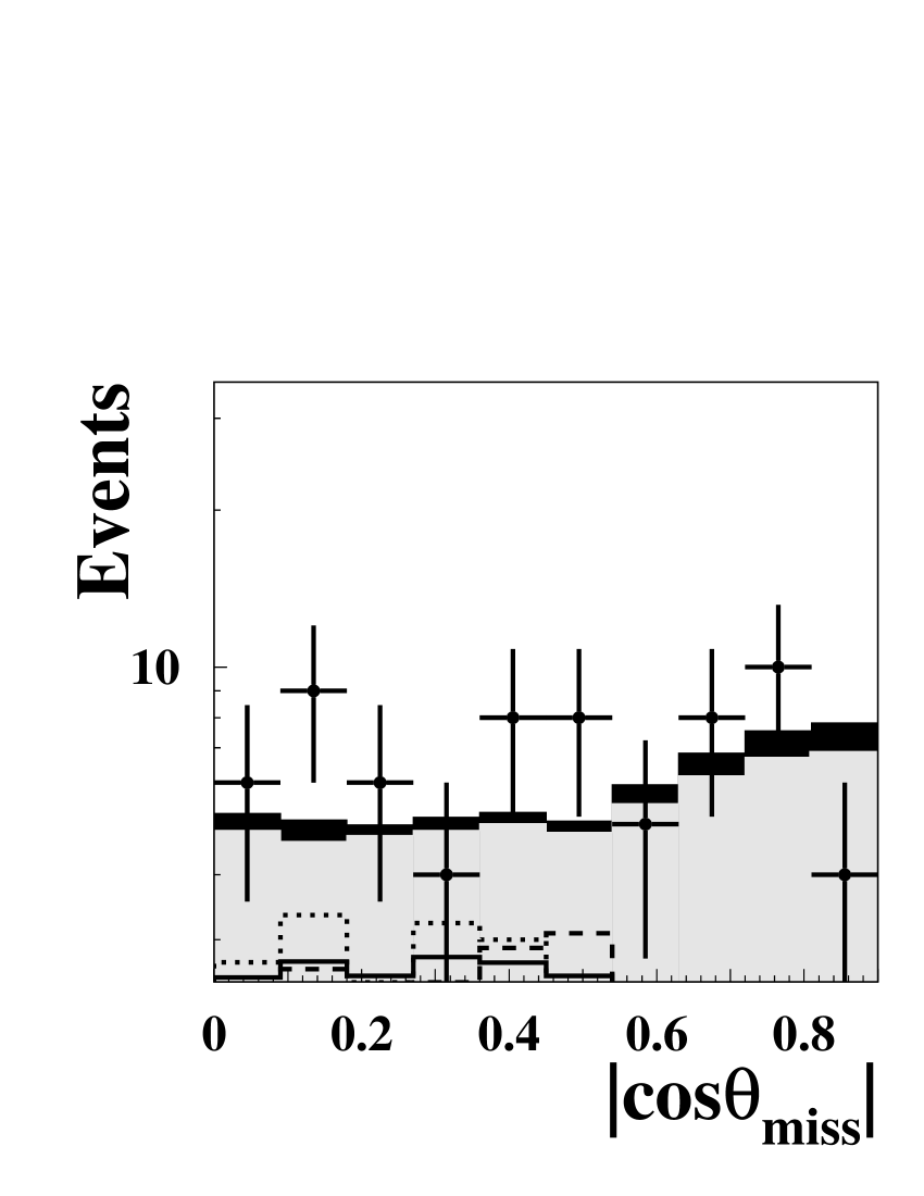
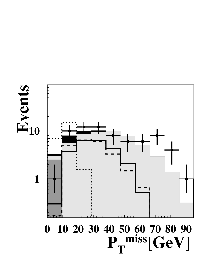
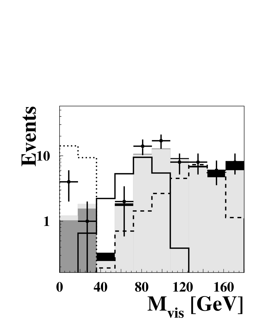
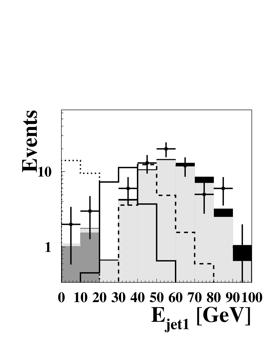
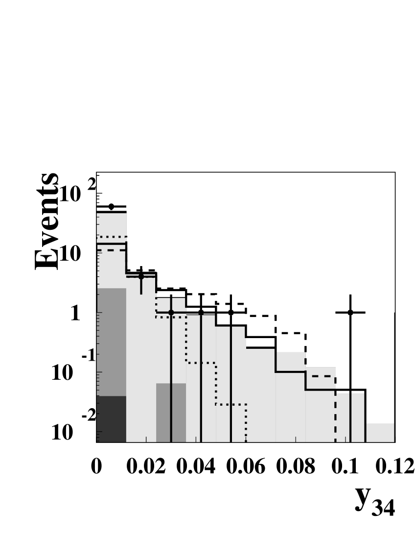
Figure 1: Comparison of data and Monte Carlo distributions of selected likelihood variables for the hadronic chargino analysis, shown at preselection level for $\sqrt{s}=206$ GeV. The shaded histograms show the various expected backgrounds (the darkest shades are two-fermion processes, predominantly $\mbox{$\mathrm{q}$}{\bar{\mbox{$\mathrm{q}$}}}$, the intermediate grey represents the two-photon contribution and the light grey indicates the dominant four-fermion background) and the points with error bars are the OPAL data. The dashed empty histograms show a sample signal with $(M,\Delta M)=$(100 GeV, 76.9 GeV), the empty histograms with the solid line show a sample signal with $(M,\Delta M)=$(100 GeV, 49.2 GeV), and the dotted empty histograms show a sample signal with $(M,\Delta M)=$(100 GeV, 12.2 GeV), all with arbitrary normalization.

Likelihood distributions are shown for the signal, expected background and observed data for two pairings of $(M,\Delta M)$ in Figure 2.

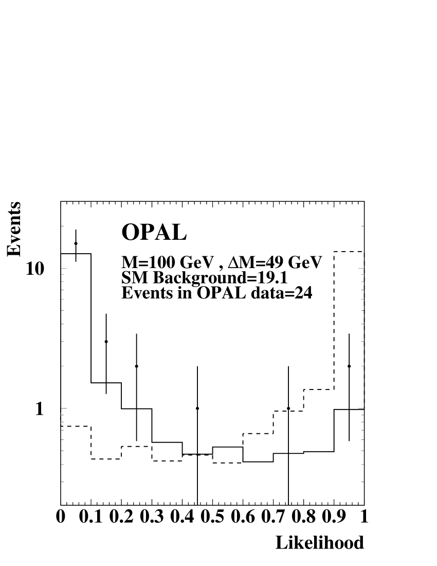
Figure 2: Sample distributions of $L_{R}$ for Standard Model background in the hadronic channel (solid histogram), chargino signal with arbitrary normalization (dashed histogram) and OPAL data at $\sqrt{s}=207$ GeV (points with error bars) at $(M,\Delta M)=$ (100 GeV, 49 GeV) and (100 GeV, 77 GeV).

3.4 Chargino Pair Production Semileptonic Selection

The event topology for the semileptonic channel consists of two jets, a lepton and an amount of missing energy which is dependent on $\Delta M$. The principal backgrounds are ${\mbox{$\mathrm{W}$}}^{+}{\mbox{$\mathrm{W}$}}^{-}\to{\mbox{$\mathrm{q}$}}{\bar{\mbox{$\mathrm{q}$}}}\ell\nu$, two-photon processes leading to ${\mbox{$\mathrm{e}$}}^{+}{\mbox{$\mathrm{e}$}}^{-}{\mbox{$\mathrm{q}$}}{\bar{\mbox{$\mathrm{q}$}}}$ and ${\mbox{$\mathrm{e}$}}^{+}{\mbox{$\mathrm{e}$}}^{-}\tau^{+}\tau^{-}$ final states, $\tau^{+}\tau^{-}$ with at least one of the taus decaying hadronically, and ${\mbox{$\mathrm{q}$}}{\bar{\mbox{$\mathrm{q}$}}}(\gamma)$ events with a lepton, usually fake, in one of the jets.

Overlap with the hadronic channel is avoided by requiring the presence in the event of an isolated lepton candidate with the same isolation criteria as in searches at lower energies [7]. Overlap with the leptonic channel is almost eliminated, as for the hadronic channel, by vetoing events which pass the selection for ${\mbox{$\mathrm{W}$}}^{+}{\mbox{$\mathrm{W}$}}^{-}\to\ell^{+}\nu\ell^{-}{\bar{\nu}}$ events of the ${\mbox{$\mathrm{W}$}}^{+}{\mbox{$\mathrm{W}$}}^{-}$ analysis.

After applying the general preselection and the veto cuts just described, the following additional cuts are made. To remove poorly reconstructed events, it is required that the event visible mass, $M_{\mathrm{vis}}$, and hadronic mass, $M_{\mathrm{had}}$, as well as the invariant mass of the system consisting of the lepton candidate and the missing momentum vector, $M_{\ell\mathrm{miss}}$, all be less than or equal to the centre-of-mass energy. Cuts are made at each $(M,\Delta M)$, as described in Section 3, to limit the accepted variable ranges to roughly the range of the signal distribution. These cuts are applied to all of the variables used for likelihood distributions, which helps to ensure that the signal reference histograms used in the likelihood have data in all bins and a smooth distribution. The same type of cut is applied to some additional variables which are not used in the likelihood because they are less powerful discriminants or because they are too strongly correlated with better variables that are already in the likelihood.

The following variables are used in the likelihood. Distributions of these variables are shown at preselection level in Figure 3.

• $M_{\mathrm{vis}}/\sqrt{s}$ discriminates against four-fermion background, especially ${\mbox{$\mathrm{W}$}}{\mbox{$\mathrm{e}$}}\nu\to{\mbox{$\mathrm{q}$}}{\bar{\mbox{$\mathrm{q}$}}}{\mbox{$\mathrm{e}$}}\nu$ with a fake lepton in one of the two jets;

• $M_{\ell\mathrm{miss}}/\sqrt{s}$ helps to reject ${\mbox{$\mathrm{W}$}}^{+}{\mbox{$\mathrm{W}$}}^{-}\to{\mbox{$\mathrm{q}$}}{\bar{\mbox{$\mathrm{q}$}}}\ell\nu$;

• the scaled magnitude of the momentum of the lepton candidate, $p_{\ell}/\sqrt{s}$, also helps to reject ${\mbox{$\mathrm{W}$}}^{+}{\mbox{$\mathrm{W}$}}^{-}\to{\mbox{$\mathrm{q}$}}{\bar{\mbox{$\mathrm{q}$}}}\ell\nu$ ;

• $M_{\mathrm{had}}/\sqrt{s}$ also helps to reject ${\mbox{$\mathrm{W}$}}^{+}{\mbox{$\mathrm{W}$}}^{-}$ events;

• $a_{T}$, the magnitude of the component of the missing momentum perpendicular to the event thrust axis, scaled to the beam energy, discriminates against two-photon and $\tau^{+}\tau^{-}$ events;

• when the event, excluding the lepton candidate, is forced into two jets, $\phi_{\mathrm{acop}}$, the acoplanarity angle of the two jets, rejects two-photon backgrounds and events with ISR;

• $|\cos\theta_{\mathrm{jet}}|$, where $\theta_{\mathrm{jet}}$ is the polar angle of the jet closer to the beam axis, rejects two-photon and two-fermion backgrounds;

• the scaled energy of the less energetic jet, $E_{\mathrm{j}}/\sqrt{s}$, helps to remove some two-fermion backgrounds and events with poorly reconstructed jets.

The following variables are used only for additional mass-dependent cuts.

• the energy of the more energetic jet, scaled to the beam energy, discriminates against four-fermion backgrounds;

• $p_{\mathrm{T}}^{\mathrm{miss}}/\sqrt{s}$, discriminates against two-photon backgrounds;

• $|\cos\theta_{a}|$, where $\theta_{a}$ is the polar angle of the $a_{T}$ vector, rejects two-photon and $\tau^{+}\tau^{-}$ backgrounds;

• $|\cos{\theta_{\mathrm{miss}}}|$ rejects two-photon and ISR events.

Signal efficiencies for semileptonic events after these additional cuts, including the cuts on the likelihood variables, vary from about 0.08% at $\Delta M=3$ GeV to about 30% for $5\mbox{ GeV}<\Delta M<10\mbox{ GeV}$ to about 60% for $\Delta M>10$ GeV. The main background surviving after the cuts in the region where $\Delta M>10$ GeV comes from four-fermion processes with a cross-section of about 1 – 2.5 pb. About 0.5 – 0.7 pb of ${\mbox{$\mathrm{e}$}}^{+}{\mbox{$\mathrm{e}$}}^{-}\tau^{+}\tau^{-}$ two-photon events survive for all values of $\Delta M$ and this is the dominant background for $\Delta M<10$ GeV. There are also about 0.05 – 0.1 pb of ${\mbox{$\mathrm{e}$}}^{+}{\mbox{$\mathrm{e}$}}^{-}{\mbox{$\mathrm{q}$}}{\bar{\mbox{$\mathrm{q}$}}}$ two-photon events for all $\Delta M$ and about 0.1 pb each of tau pairs and ${\mbox{$\mathrm{q}$}}{\bar{\mbox{$\mathrm{q}$}}}(\gamma)$ events for $\Delta M>10$ GeV.

OPAL

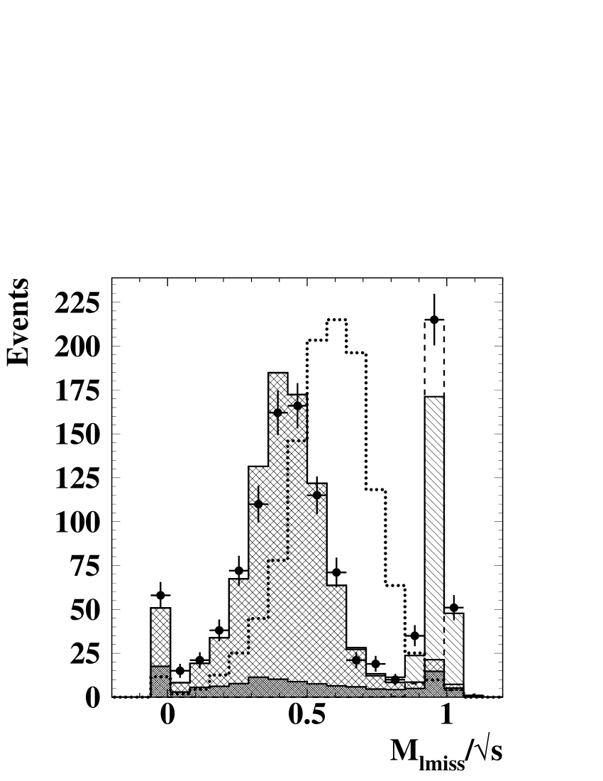
Figure 3: Comparison of data and Monte Carlo distributions of selected likelihood variables for the semileptonic chargino analysis, shown at preselection level for $\sqrt{s}=207$ GeV. The solid histograms represent the expected background, with dark grey for two-fermion events, cross-hatching for four-fermion events and single-hatching for two-photon events. The points with error bars are the OPAL data taken in the year 2000 at an average centre-of-mass energy of 206.1 GeV. Dotted histograms show a “$\mbox{$\mathrm{W}$}^{+}\mbox{$\mathrm{W}$}^{-}$-like” signal with $(M,\Delta M)=$(80 GeV, 76.3 GeV) and dashed histograms show a “two-photon–like” signal with $(M,\Delta M)=$(85 GeV, 6.9 GeV), both with arbitrary normalization.

Some examples of likelihood distributions are shown in Figure 4 for signal, data and expected Standard Model background.

Figure 4: Sample distributions of $L_{R}$ for Standard Model background in the semileptonic channel (solid histogram), chargino signal with arbitrary normalization (dashed histogram) and OPAL data at $\sqrt{s}=207$ GeV (points with error bars) at $(M,\Delta M)=$ (76 GeV, 70 GeV) and (100 GeV, 48 GeV).

3.5 Neutralino Associated Production Hadronic Selection

The final state topology for $\tilde{\chi}^{0}_{2}\tilde{\chi}^{0}_{1}$ production with a hadronic decay of the virtual ${\mbox{$\mathrm{Z}$}}^{0}$ contains two hadronic jets and missing energy from the two stable lightest neutralinos in the final state. The analysis is very similar to the hadronic decay channel analysis for chargino pair production. Some changes are made to reflect the difference in event topology. The following variables are used:

• Cut Variables — as for the chargino analysis except that no cuts are made on the number of jets in the event, on $E_{\ell^{\prime}}$ nor on $E_{\mathrm{jet}1}$;

• Likelihood Variables:

  • $|\cos\theta_{\mathrm{miss}}|$, $p_{\mathrm{T}}^{\mathrm{miss}}$, $\phi_{\mathrm{acop}}$ and $M_{\mathrm{vis}}$ are used, as for the hadronic channel of the chargino analysis;

  • $R_{\mathrm{fwd}}^{\mathrm{vis}}$, the ratio of energy deposited in the forward region, $|\cos\theta|>0.9$, to the total visible energy, helps to remove ISR and two-photon events;

  • $M_{\mathrm{vis}}/E_{\mathrm{vis}}$, the ratio of the visible invariant mass to the total visible energy gives a measure of the “softness” and helps to remove ${\mbox{$\mathrm{q}$}}{\bar{\mbox{$\mathrm{q}$}}}\nu{\bar{\nu}}$ events;

  • $d_{23}\equiv\sqrt{y_{23}E_{\mathrm{vis}}^{2}}$, helps to remove backgrounds containing more than two jets.

4 Extended Likelihood Method, Combination of Channels and Energies

Once the discriminant value $L_{R}$ has been calculated for all events, as described in Section 3, it can be used either in an optimized cut analysis or in an “extended” likelihood analysis, as described in [8]. The optimized cut analysis has the disadvantage of being difficult to use effectively in a search such as this one, where the signal cross-section and hence the signal purity are unknown, and the number of selected events is sensitive to the position of the cut so that small modifications to the analysis can occasionally have a very large effect on the limits obtained.

In the case of an unknown signal cross-section, an “extended” likelihood technique is more appropriate, as it is optimal for all luminosities and signal cross-sections. In this case, the distributions of the discriminant $L_{R}$ are evaluated for signal and background samples and the value of $L_{R}$ is evaluated for each data event. A single likelihood $L$ can then be constructed which describes the probability, given the signal and background $L_{R}$ distributions $S$ and $B$, of observing $N$ events passing all cuts with likelihoods $L_{R_{i}}$:

$$L=\frac{e^{-\nu}\nu^{N}}{N!}\prod^{N}_{i=1}P(L_{R_{i}}|B,S)$$ (1)

where $\nu\equiv\mu_{B}+\epsilon{\cal L}\omega\sigma_{S}$ is the expected number of background events passing the cuts, $\mu_{B}$, plus the expected number of preselected signal events for a signal cross-section $\sigma_{S}$, and integrated luminosity ${\cal L}$, assuming signal efficiency $\epsilon$. In the extended likelihood method, efficiencies are evaluated at the end of the cut-based selection. All candidates passing the preselection and additional cuts contribute to the final limit calculation, with weights given by their likelihood of being signal. There is no cut on the likelihood value, and therefore no sensitivity to cut position, making the limit very robust.

A weighting factor, $\omega=\frac{\sigma(\sqrt{s_{i}})}{\sigma(\sqrt{s_{\mathrm{limit}}})}$, is included to allow the cross-section limit to be set at a particular centre-of-mass energy using data taken at many different energies. Since charginos and neutralinos are fermions, $\sigma$ is assumed to scale as $\beta/s$. With some algebraic manipulation [8] Equation 1 can be rewritten in the form:

$$\ln{L(\sigma_{S})}=-(\mu_{B}+\epsilon{\cal L}\omega\sigma_{S})+\sum^{N}_{i=1}\ln[\mu_{B}B(L_{R_{i}})+\epsilon{\cal L}\omega\sigma_{S}S(L_{R_{i}})]$$ (2)

This can be calculated separately for each channel with data taken at several centre-of-mass energies. The 95% confidence level limit on the signal cross-section $\sigma_{S}(\sqrt{s_{\mathrm{limit}}})$ at $\sqrt{s_{\mathrm{limit}}}=208$ GeV is computed using Bayes’ theorem with a uniform prior in $\sigma_{S}$ by solving:

$$0.95=\frac{{\displaystyle\int_{0}^{\sigma_{95}^{\mathrm{limit}}}}\prod_{i=1}^{N_{{\mathrm{channels}},\sqrt{s}}}L_{i}(\sigma_{S}^{\mathrm{limit}})\mathrm{d}\sigma_{S}^{\mathrm{limit}}}{{\displaystyle\int_{0}^{\infty}}\prod_{i=1}^{N_{{\mathrm{channels}},\sqrt{s}}}L_{i}(\sigma_{S}^{\mathrm{limit}})\mathrm{d}\sigma_{S}^{\mathrm{limit}}}$$ (3)

Limits on the signal cross-sections are calculated according to Equation 3 separately for each channel in the chargino analysis and for all channels combined assuming 100% ${\mbox{$\mathrm{W}$}}^{\ast}$ branching ratios. In all cases, all the energy bins from Table 2 are combined. Data from a particular centre-of-mass energy contribute to the combination only up to the kinematic cut-off for that energy, about $(\sqrt{s}-1\mbox{ GeV})/2$. These cut-offs are then rounded down to the nearest 0.5 GeV. Thus, all data with energies above 192 GeV contribute up to a chargino mass of 95.5 GeV, only those with energies above 196 GeV contribute up to 97.5 GeV and so on until the limit for chargino masses between 103 and 103.5 GeV comes only from the data taken at an average centre-of-mass energy of 208 GeV. The limit is calculated on the cross-section at $\sqrt{s_{\mathrm{limit}}}=208$ GeV.

For points where the background likelihood histograms contain empty bins, the extended likelihood method cannot be used and a simple Poisson probability is evaluated, based on the observed number of events passing the preselection and additional cuts and the number expected from background Monte Carlo. This happens for most of the points with $\Delta M<15$ GeV and for some points with $\Delta M$ between 15 and 30 GeV.

5 Systematic Errors

There are numerous possible sources of systematic errors for these analyses. In general, however, it is found that even large errors on the efficiencies and backgrounds have rather a small effect on the limits, so only the larger effects are considered. Some sources of potentially large systematic uncertainties are:

• limited Monte Carlo statistics for signal efficiency evaluation;

• limited Monte Carlo statistics for background evaluation;

• mismodelling of likelihood variables from incomplete or incorrect Monte Carlo simulation and detector calibration effects; this includes, among other things, the effect of ignoring interference between multiperipheral and other four-fermion processes containing an electron and a positron in the final state, for which a specific check was also done, and the effect was found to be negligible for the background, given the statistical errors on the multiperipheral background samples; a relative error of 5 % was assigned to the signal efficiencies;

• a further 1 % relative systematic error was assigned to the signal efficiencies to account for the uncertainty in the smoothing procedure applied to the reference histograms;

• interpolation of signal histograms to obtain a finer grid in $\Delta M$ than was generated; a test was done using Monte Carlo samples generated at intermediate values of $\Delta M$ and a relative error of 1 % was assigned to the efficiencies;

• effects of having signal generated only at three $\sqrt{s}$ to evaluate the efficiency at all energies and using rather crude $\beta/s$ models to evaluate the cross-sections of these fermionic signals at other $\sqrt{s}$ were evaluated by repeating the whole analysis using reference histograms created from signals and backgrounds generated at 196 GeV instead of 207 GeV (in the kinematic range where this was possible) and comparing the results with the standard analysis; a conservative relative error of 5 % was assigned to the efficiencies;

• uncertainties in the estimation of the integrated luminosity of about 0.2–0.3%.

The evaluation of the uncertainties due to the first three items in the list is described in detail in subsections 5.1-5.2. Detector efficiency losses due to occupancy or due to the cuts on energy in the forward detectors, which reduce the effective integrated luminosity by about 3% were included simply by reducing all integrated luminosities by 3%. The following potential sources of systematic uncertainty were also considered and found to be negligible compared with those listed above:

• effects of having two-photon background samples generated only at some of the $\sqrt{s}$ used and simply assuming that the cross-sections of these processes are proportional to $\log{s}$ to evaluate them at other energies.

• effects of using reference histograms generated at a single $\sqrt{s}$ for evaluating the likelihood at all energies; a cross-check was done using reference histograms generated at $\sqrt{s}=196$ GeV;

All errors are evaluated by estimating the uncertainties on the rates of events passing a cut, since evaluating changes in the shapes of the $L_{R}$ distributions at every point on the $(M,\Delta M)$ grid for every possible systematic is not a practical approach.

5.1 Statistical uncertainties

The statistical uncertainties on the signal efficiency and on the background estimates due to the finite number of Monte Carlo events generated are evaluated after the preselection and additional cuts for each mass grid point.

The most important sources of background are four-fermion final states, ${\mbox{$\mathrm{q}$}}{\bar{\mbox{$\mathrm{q}$}}}(\gamma)$ and $\tau^{+}\tau^{-}$ two-fermion final states, and two-photon processes, principally ${\mbox{$\mathrm{e}$}}^{+}{\mbox{$\mathrm{e}$}}^{-}\tau^{+}\tau^{-}$ and untagged ${\mbox{$\mathrm{e}$}}^{+}{\mbox{$\mathrm{e}$}}^{-}{\mbox{$\mathrm{q}$}}{\bar{\mbox{$\mathrm{q}$}}}$. The statistical errors on the two- and four-fermion final states are very small, since the integrated luminosity of the generated Monte Carlo is about 50 to 100 times the integrated data luminosity at most centre-of-mass energies; however, the two-photon processes have very large cross-sections and it was only possible to generate about 8 to 15 times the integrated data luminosity. The statistical errors on each background are then added in quadrature to obtain the statistical error on the total background at each mass grid point for each centre-of-mass energy and in each analysis channel. The statistical errors on the background are therefore relatively high in the low $\Delta M$ region, which is dominated by two-photon processes, and almost negligible for $\Delta M>10$ GeV.

5.2 Uncertainties due to variable mismodelling

Systematic uncertainties due to differences between the data from the OPAL detector and the Monte Carlo models are estimated after an optimized cut on $L_{R}$. The $L_{R}$ cut is optimized by selecting the bin boundary on the $L_{R}$ distributions for signal and background which gives the smallest expected value of $N_{95}$ (the most signal events there could be, at a confidence level of 95%, given the expected signal and background distributions and assuming a number of observed events equal to the expected number of background events). The cut is optimized for the default $L_{R}$ distributions, and the number of events passing it is evaluated with modified $L_{R}$ distributions made from reference histograms where variables have been shifted or smeared, to determine the systematic effects on the expected background levels if the background Monte Carlo differed from the data.

For the evaluation of systematic effects due to variable mismodelling, reference histograms of the likelihood variables are constructed after the general preselection, with none of the additional mass-dependent cuts. Histograms for the sum of all the expected backgrounds are compared with histograms of the data. The peaks in the histograms are fitted with Gaussians for both the data and the Monte Carlo. The differences between the peaks are compared with the statistical uncertainties on each background. If a distribution has two peaks and one is due mainly to two-photon events and the other mainly to four-fermion events, which can be determined by looking at the Monte Carlo data for each background individually, the comparison for each background is made only for the relevant peak. No attempt was made to apply this procedure to the variables with obviously non-Gaussian distributions, such as cosine distributions; their shapes generally show good agreement between data and Monte Carlo. If the difference in peak position is larger than the statistical uncertainty for a particular background, then the difference minus the statistical uncertainty is taken to be the systematic uncertainty, and reference histograms are constructed for each background with the variable shifted by the amount given by this prescription. A similar procedure is applied to the comparison of the widths of the peaks in data and Monte Carlo and used to determine an amount by which to smear the variables for the reference histograms. When these are compared with quantities obtained by comparing OPAL ${\mbox{$\mathrm{Z}$}}^{0}$ data with Monte Carlo, which allows a comparison which is not statistically limited, agreement is reasonably good.

5.3 Method for extrapolating systematic uncertainty estimates to the full mass grid

Variations due to systematic uncertainties are evaluated at a centre-of-mass energy of 207 GeV, which allows mass grid points near the kinematic limit to be considered, and is an energy at which both signal and background Monte Carlo samples are available. It is assumed that the uncertainties at 207 GeV are typical and can be used at all centre-of-mass energies. The errors are evaluated at three mass grid points: $(M_{\chi^{\pm}}=80.0\,{\mathrm{GeV}},\Delta M=76.3\,{\mathrm{GeV}})$, where signal events give a final state topology almost identical to that of on-shell $\mathrm{W}$-pair production, $(M_{\chi^{\pm}}=85.0\,{\mathrm{GeV}},\Delta M=6.9\,{\mathrm{GeV}})$, where the detected particles from signal events are very soft and the main background is from two-photon events, and $(M_{\chi^{\pm}}=100.0\,{\mathrm{GeV}},\Delta M=49.2\,{\mathrm{GeV}})$, which is near the kinematic limit and has background coming from both four-fermion and two-fermion production. Uncertainties are estimated for each of the main background sources at each of these points. The difference between the result with the smear or shift and the original result is found and the statistical uncertainty for that background subtracted off. These differences are then summed in quadrature for the shifts and smears of all the variables. The errors at the three points are then compared and, in general, the error from the most relevant of the three for the particular background is chosen to be the error; in other words, the errors on the four-fermion background are generally taken from the point $(M_{\chi^{\pm}}=80.0\,{\mathrm{GeV}},\Delta M=76.3\,{\mathrm{GeV}})$, while the errors on two-photon backgrounds come from the point $(M_{\chi^{\pm}}=85.0\,{\mathrm{GeV}},\Delta M=6.9\,{\mathrm{GeV}})$.

Table 4: Relative systematic errors on major backgrounds in the semileptonic channel for the chargino analysis.

Background	Relative
Source	Systematic Error
${\mbox{$\mathrm{q}$}}{\bar{\mbox{$\mathrm{q}$}}}$	0.48
$\tau^{+}\tau^{-}$	0.19
4-fermion	0.25
${\mbox{$\mathrm{e}$}}^{+}{\mbox{$\mathrm{e}$}}^{-}\mu^{+}\mu^{-}$	1.0
${\mbox{$\mathrm{e}$}}^{+}{\mbox{$\mathrm{e}$}}^{-}\tau^{+}\tau^{-}$	0.95
${\mbox{$\mathrm{e}$}}^{+}{\mbox{$\mathrm{e}$}}^{-}{\mbox{$\mathrm{q}$}}{\bar{\mbox{$\mathrm{q}$}}}$	1.0

The results of this study are used to give the relative systematic errors shown in Tables 4 and 5.

Table 5: Relative systematic errors on major backgrounds in the hadronic channel for the chargino and neutralino analyses.

Background	Relative
Source	Systematic Error
${\mbox{$\mathrm{q}$}}{\bar{\mbox{$\mathrm{q}$}}}$	0.3
4-fermion	0.8
${\mbox{$\mathrm{e}$}}^{+}{\mbox{$\mathrm{e}$}}^{-}{\mbox{$\mathrm{q}$}}{\bar{\mbox{$\mathrm{q}$}}}$	0.5

The fractional contribution of each background was then calculated for the rest of the mass grid and the relative errors on each background scaled according to the contribution of that background at each point. The systematic errors for each background at each grid point are then added in quadrature and eventually summed in quadrature with the statistical error on the background. The efficiency errors are summed in quadrature and a total relative systematic error of 7% is applied to the signal efficiencies and summed in quadrature with the statistical uncertainties.

5.4 Incorporating uncertainties into cross-section limits

Once the systematic errors have been evaluated for the signal efficiency and background expectation at every point on the mass grid for all energies, the limit setting code is run twice more over the data: once with all the efficiencies decreased by their errors and all background expectations increased by their errors to give the worst expected sensitivity, and once with the efficiencies increased and backgrounds decreased to give the best expected sensitivity. There are then three limits for each point in the grid: the standard one, $L95_{0}$, the one standard deviation “worst case” one, $L95_{+}$, and the one standard deviation “best case” one, $L95_{-}$. All are evaluated at a centre-of-mass energy of 208 GeV. A Gaussian-weighted average of these gives the limit convolved with the systematic errors:

$$L95=\frac{L95_{0}+\frac{1}{\sqrt{e}}(L95_{+}+L95_{-})}{1+\frac{2}{\sqrt{e}}}.$$ (4)

This is a three-point integral; it is a simple and robust way to deal with large errors, which tend to make more complex methods unstable. Despite the large relative errors on the background expectation, the limits typically change by only about 0.001–0.02 pb, with an increase of about 0.1 pb for the hadronic channel in the “${\mbox{$\mathrm{W}$}}^{+}{\mbox{$\mathrm{W}$}}^{-}$” region where $(M,\Delta M)\approx(80\,\mathrm{GeV},80\,\mathrm{GeV})$ and an increase of several picobarns along the $\Delta M=3$ GeV “two-photon” strip for the semileptonic channel.

6 Final cross-section limits

In order to give a visual impression of what the limits might look like in the absence of a signal, “expected” limits are calculated. For each point on the mass grid, an average is made of the cross-section limits from a hundred toy Monte Carlo experiments. In each experiment, a random number of “events” is generated using a Poisson distribution with a mean value of $\mu_{B}$, the expected number of background events for the mass grid point. Each “event” is assigned a random likelihood $L_{R_{i}}$ from the background likelihood distribution $B(L_{R_{i}})$. The signal cross-section limit is then calculated just as it is for the data.

6.1 Chargino Pair Production, Hadronic channel

The limit observed is in general slightly higher than the expected limit; however, the 95% confidence level limit on $\sigma_{\tilde{\chi}^{+}_{1}\tilde{\chi}^{-}_{1}}BR^{2}(\tilde{\chi}^{\pm}_{1}\to{\mbox{$\mathrm{q}$}}{\bar{\mbox{$\mathrm{q}$}}}\tilde{\chi}^{0}_{1})$ (shown in Figure 5) is below about 0.3 pb almost up to the kinematic limit for $\Delta M<3$ GeV and well below 0.1 pb in most of the parameter space explored, whereas a chargino signal would be expected to have a cross-section of several picobarns.

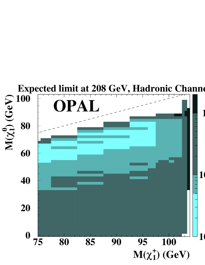
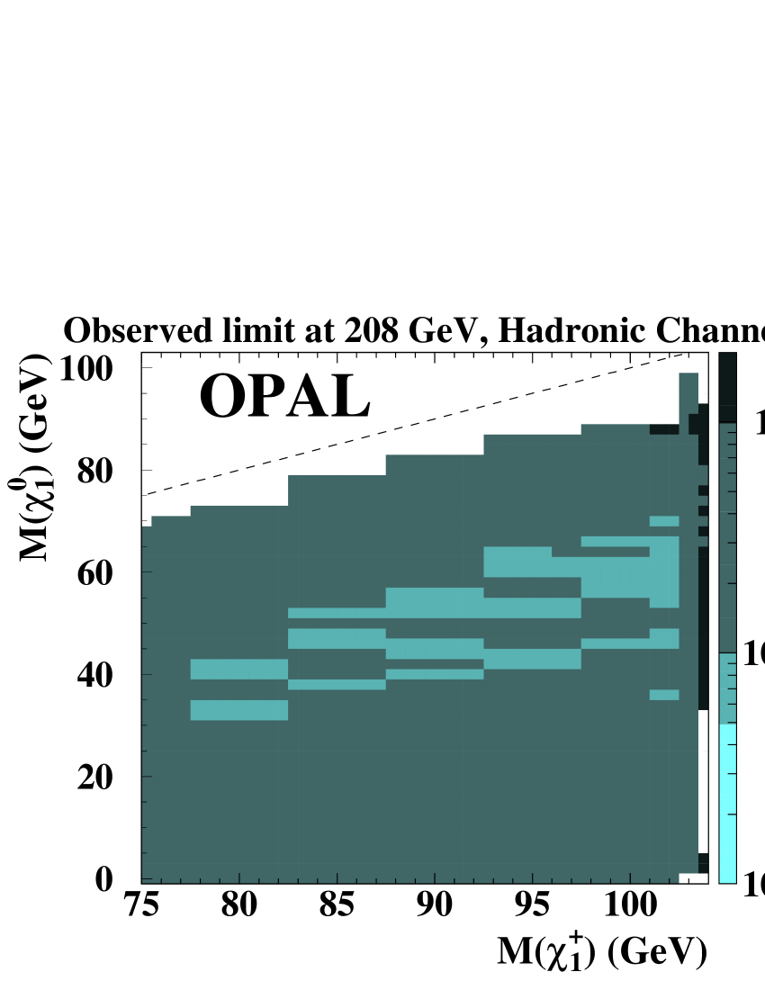
Figure 5: The expected and observed 95% confidence level limits on $\sigma({\mbox{$\mathrm{e}$}}^{+}{\mbox{$\mathrm{e}$}}^{-}\to\tilde{\chi}^{+}_{1}\tilde{\chi}^{-}_{1})BR^{2}(\tilde{\chi}^{\pm}\to q{\bar{q}}\tilde{\chi}^{0}_{1})$, using data taken at 192-209 GeV. White areas indicate that the limit is greater than 2 pb or that no limit could be set.

6.2 Chargino Pair Production, Semileptonic channel

The observed limits are not as stringent as the expected ones; however, the 95% confidence level limit on $\sigma_{\tilde{\chi}^{\pm}_{1}\tilde{\chi}^{\pm}_{1}}BR(\tilde{\chi}^{\pm}_{1}\to{\mbox{$\mathrm{q}$}}{\bar{\mbox{$\mathrm{q}$}}}\tilde{\chi}^{0}_{1})BR(\tilde{\chi}^{\pm}_{1}\to\ell\nu\tilde{\chi}^{0}_{1})$ (shown in Figure 6) is below about 0.3 pb almost up to the kinematic limit for $\Delta M<3$ GeV and well below 0.1 pb in much of the parameter space explored.

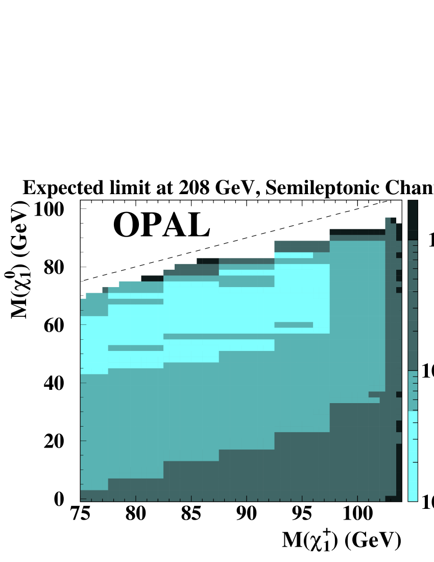
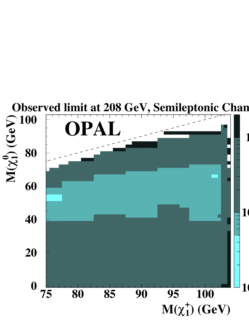
Figure 6: The expected and observed 95% confidence level limits on the cross-section for the final state containing jets and a lepton with missing energy, using data taken at 192-209 GeV. White areas indicate that the limit is greater than 2 pb or that no limit could be set.

6.3 Chargino Pair Production, Leptonic channel

The observed 95% confidence level limits on $\sigma_{\tilde{\chi}^{\pm}_{1}\tilde{\chi}^{\pm}_{1}}BR^{2}(\tilde{\chi}^{\pm}_{1}\to\ell\nu\tilde{\chi}^{0}_{1})$ taken from [4] are shown in Figure 7 and are slightly better than the expected limits.

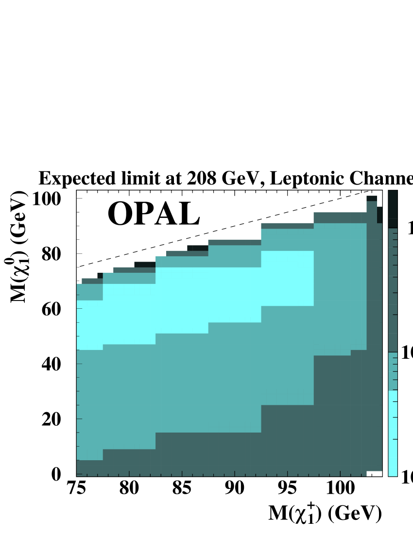
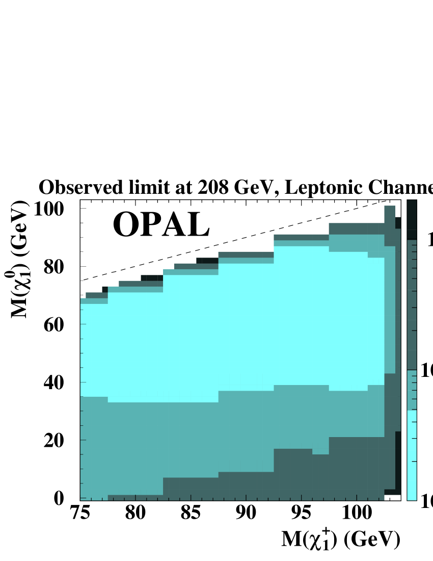
Figure 7: The expected and observed 95% confidence level limits on the product of the cross-section for chargino pair production and the square of the branching ratio for $\tilde{\chi}^{\pm}$ to leptons and missing energy, using data taken at 192-209 GeV. White areas indicate that the limit is greater than 2 pb or that no limit could be set.

6.4 Chargino Pair Production, Channels Combined Assuming 100% ${\mbox{$\mathrm{W}$}}^{\pm}$ Branching Ratios

If the lightest neutralino is the LSP, chargino branching ratios to final states containing ${\mbox{$\mathrm{q}$}}{\bar{\mbox{$\mathrm{q}$}}}$ and $\ell\nu$ are the ${\mbox{$\mathrm{W}$}}^{\pm}$ decay branching ratios, except for very low values of $\Delta M$ where the leptonic branching ratio increases rapidly. The three channels are combined according to ${\mbox{$\mathrm{W}$}}^{\pm}$ branching ratios and these results, which are generally valid in the absence of light scalar leptons and scalar neutrinos, are shown in Figure 8.

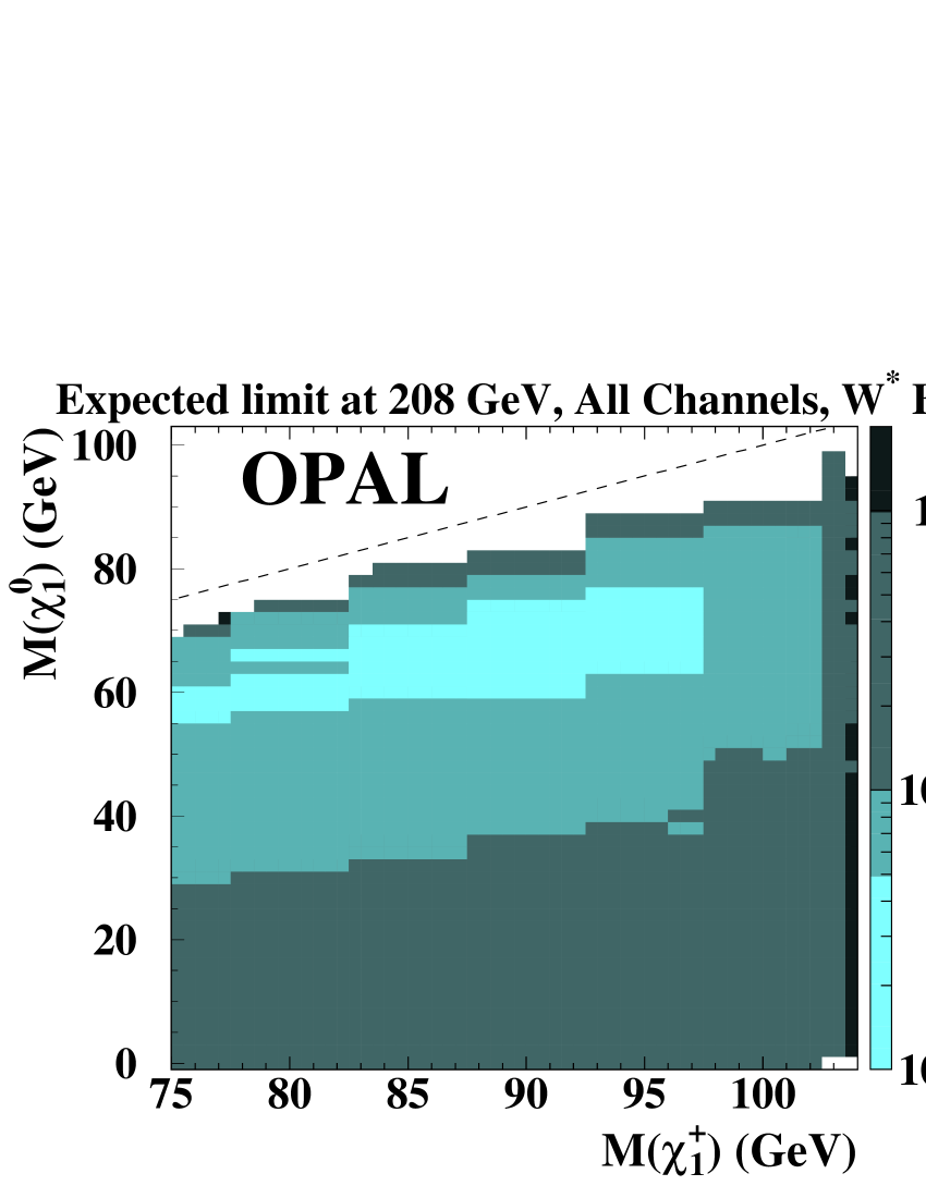
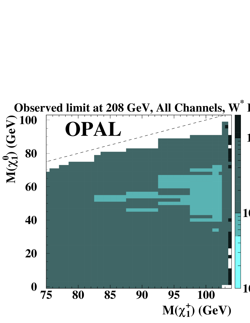
Figure 8: The expected and observed 95% confidence level limits on the cross-section for chargino pair production, assuming 100% ${\mbox{$\mathrm{W}$}}^{\ast}$ branching ratios for the chargino decays and using all the data sets analyzed. White areas indicate that the limit is greater than 2 pb or that no limit could be set.

6.5 Neutralino Associated Production, Hadronic Channel

Since only the hadronic channel was analyzed for neutralino associated production, the results are presented both as a limit on $\sigma_{\tilde{\chi}^{0}_{2}\tilde{\chi}^{0}_{1}}BR(\tilde{\chi}^{0}_{2}\to{\mbox{$\mathrm{q}$}}{\bar{\mbox{$\mathrm{q}$}}}\tilde{\chi}^{0}_{1})$ (Figure 9) and as a limit on $\sigma_{\tilde{\chi}^{0}_{2}\tilde{\chi}^{0}_{1}}$ assuming 100% ${\mbox{$\mathrm{Z}$}}^{0\ast}$ branching ratios for $\tilde{\chi}^{0}_{2}$ decay (Figure 10). The 95% confidence level limit on the cross-section is less than 0.1 pb for $\Delta M>5$ GeV to within about a GeV of the kinematic limit. There is no value of $(M(\tilde{\chi}^{0}_{2}),M(\tilde{\chi}^{0}_{1}))$ for which a significant excess is observed.

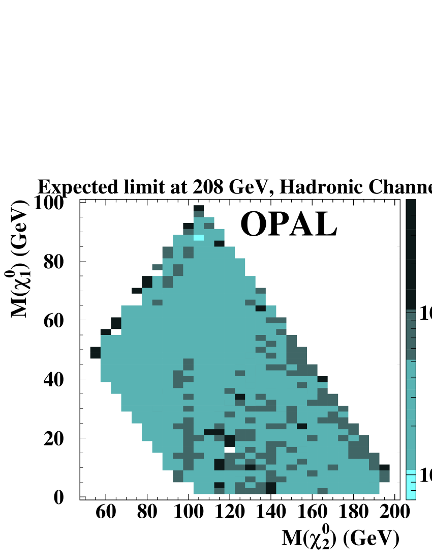
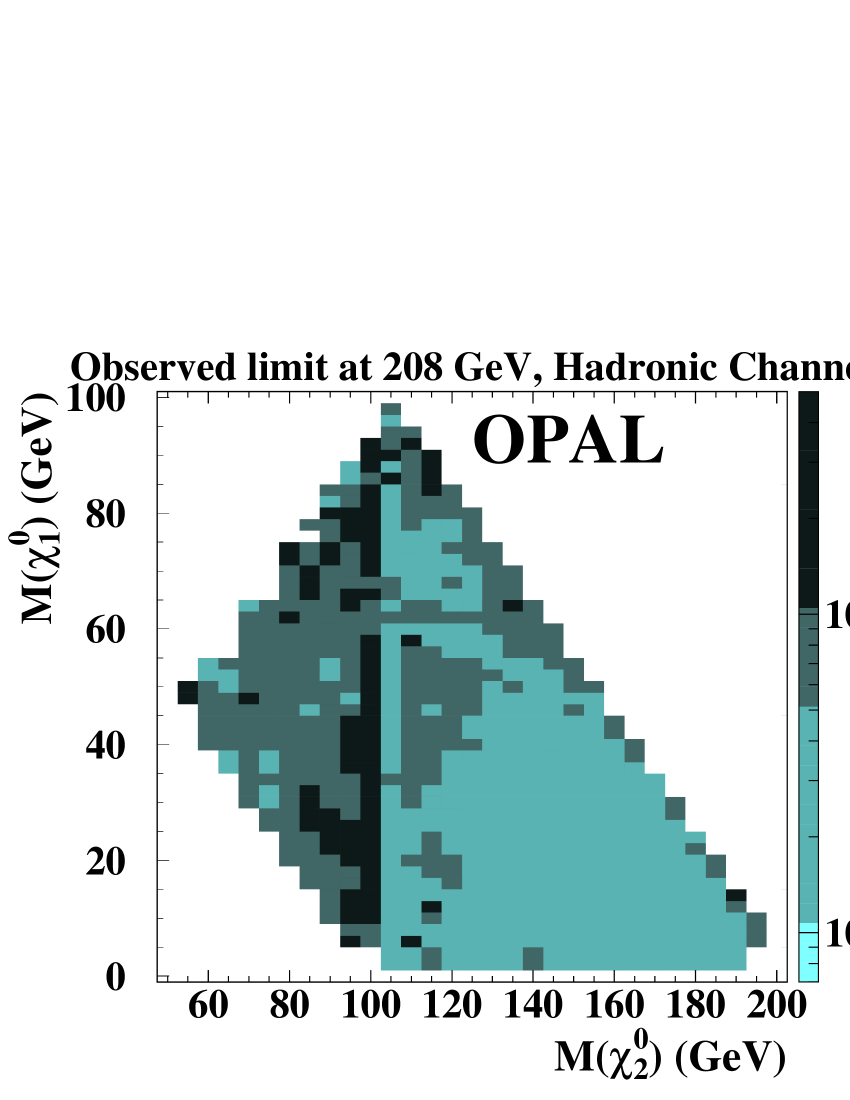
Figure 9: The expected and observed 95% confidence level limits on the product of the cross-section for $\tilde{\chi}^{0}_{2}\tilde{\chi}^{0}_{1}$ associated production and the branching ratio for $\tilde{\chi}^{0}_{2}\to{\mbox{$\mathrm{q}$}}{\bar{\mbox{$\mathrm{q}$}}}\tilde{\chi}^{0}_{1}$ decays. No signal Monte Carlo events were generated with $M_{\tilde{\chi}^{0}_{2}}+M_{\tilde{\chi}^{0}_{1}}<100$ GeV, so no limit is evaluated in this region. White areas indicate that the limit is greater than 0.5 pb or that no limit could be set.

Figure 10: The expected and observed 95% confidence level limits on the cross-section for $\tilde{\chi}^{0}_{2}\tilde{\chi}^{0}_{1}$ associated production, based on decays to hadronic final states and assuming 100% ${\mbox{$\mathrm{Z}$}}^{0\ast}$ branching ratios for the $\tilde{\chi}^{0}_{2}$ decays. No signal Monte Carlo events were generated with $M_{\tilde{\chi}^{0}_{2}}+M_{\tilde{\chi}^{0}_{1}}<100$ GeV, so no limit is evaluated in this region. White areas indicate that the limit is greater than 0.5 pb or that no limit could be set.

Despite the small general excess which results in larger than expected cross-section limits in the hadronic and semileptonic channels, there is no indication of chargino or neutralino production in the OPAL data.

7 Interpretation in the Constrained MSSM

The experimental information required to obtain limits in any particular model is contained in the cross-section limit for chargino production as a function of the leptonic branching ratio and in the cross-section limit for neutralino associated production as a function of the invisible branching ratio. Comparing the limits with the cross-section and leptonic branching fraction predicted by any specific model allows that model to be tested with the OPAL data.

In this section, the results are interpreted in the context of the Contrained Minimal Supersymmetric Standard Model (CMSSM). This is a model inspired by Minimal Supergravity, in which it is assumed that at some large Grand Unification (GUT) scale all of the gauginos have a common mass $m_{1/2}$. This implies that there is a fixed relation between the three gaugino masses at the electroweak scale, $M_{1}$ for $U(1)$ partners, $M_{2}$ for $SU(2)$ partners, and $M_{3}$ for $SU(3)$ partners, so a single free parameter, taken to be $M_{2}$, generates all the gaugino masses. It is also assumed that the sfermions (but not all scalars as in true Minimal Supergravity) have a common mass at the SUSY-breaking scale, denoted by $m_{0}$. With these constraints, there are only six free parameters not present in the SM: $M_{2}$, $m_{0}$, the common trilinear sfermion-Higgs coupling at the Planck scale $A_{0}$, the ratio of the two vacuum expectation values for the Higgs doublet fields coupling to down- and up-type quarks $\tan\beta$, the mass mixing parameter of the Higgs fields $\mu$, and the mass of the pseudoscalar Higgs boson $m_{A}$. With these six parameters, it is possible to calculate cross-sections for $\chi^{+}_{1}\chi^{-}_{1}$ and $\chi^{0}_{2}\chi^{0}_{1}$ production.

The properties of the charginos and neutralinos depend chiefly on $M_{2}$, $\mu$ and $\tan\beta$. If $M_{2}\gg|\mu|$, then the lightest neutralino is higgsino-like and $t$-channel contributions are negligible; the $\chi^{\pm}_{1},\chi^{0}_{1}$ and $\chi^{0}_{2}$ are all close in mass and the cross-section for $\chi^{0}_{2}\chi^{0}_{1}$ production is similar to that of $\chi^{+}_{1}\chi^{-}_{1}$ production. If $M_{2}\ll|\mu|$ then the $\chi^{0}_{1}$ is gaugino-like; $t$-channel processes are important and may interfere destructively with the $s$-channel. Scans over $M_{2}$ and $\mu$ are done at several values of $\tan\beta$. The $m_{0}$ and $A_{0}$ parameters determine the masses of the sfermions. Results here are shown for $m_{0}=500\mbox{ GeV}$, implying that there are no light sleptons or sneutrinos, and two-body decays of charginos to $\ell^{\pm}\tilde{\nu}$ can be ignored, and for $A_{0}=0$, which generally means that mixing of left- and right-handed sfermion eigenstates is assumed to be small. A scan is performed with SUSYGEN [33] over the region $0<M_{2}<5000$ GeV, $-1000\mbox{ GeV}<\mu<1000\mbox{ GeV}$ at $\tan\beta=1,2,5,10,40$. The granularity of the scan depends on the region and is generally between 1 and 5 GeV in $M_{2}$ and $\mu$.

The simplest thing to do with the cross-section limits obtained in the previous section and the results of the CMSSM scan is to see what regions of the parameter space are excluded. By construction, the three chargino channels do not use the same events, so the best way to use this information is to sum the limits for the three channels according to the branching ratios predicted by SUSYGEN for a particular set of $M_{2},\mu,\tan\beta$ values and compare with the SUSYGEN prediction for the chargino total cross-section. The events selected in the neutralino associated production search may overlap with the events selected in the chargino search, so the optimal way to include both searches is to calculate whether the expected limit for the chargino or the neutralino search would give the better exclusion for a particular $M_{2},\mu,\tan\beta$, and use the channel which is expected to be better. Exclusions in the $M_{2},\mu$ plane are shown in figure 11 for the five values of $\tan\beta$ studied. These exclusions are valid only for $m_{0}\geq 500$ GeV and for $A_{0}=0$. The regions which are shown as kinematically accessible but not excluded correspond to regions where $\tilde{\chi}^{0}_{2}\tilde{\chi}^{0}_{1}$ production is possible, but with an expected cross-section too small to be excluded.

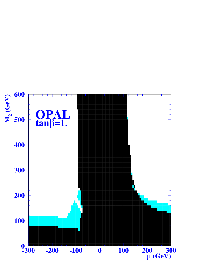
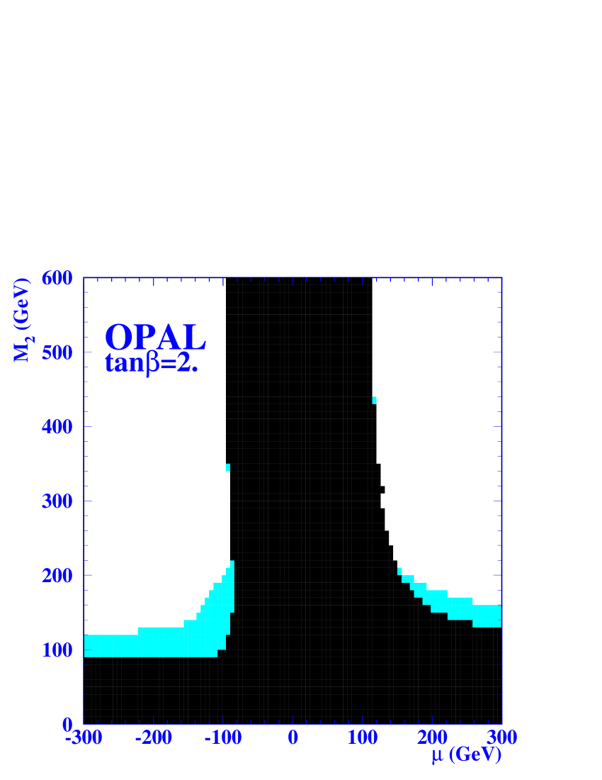
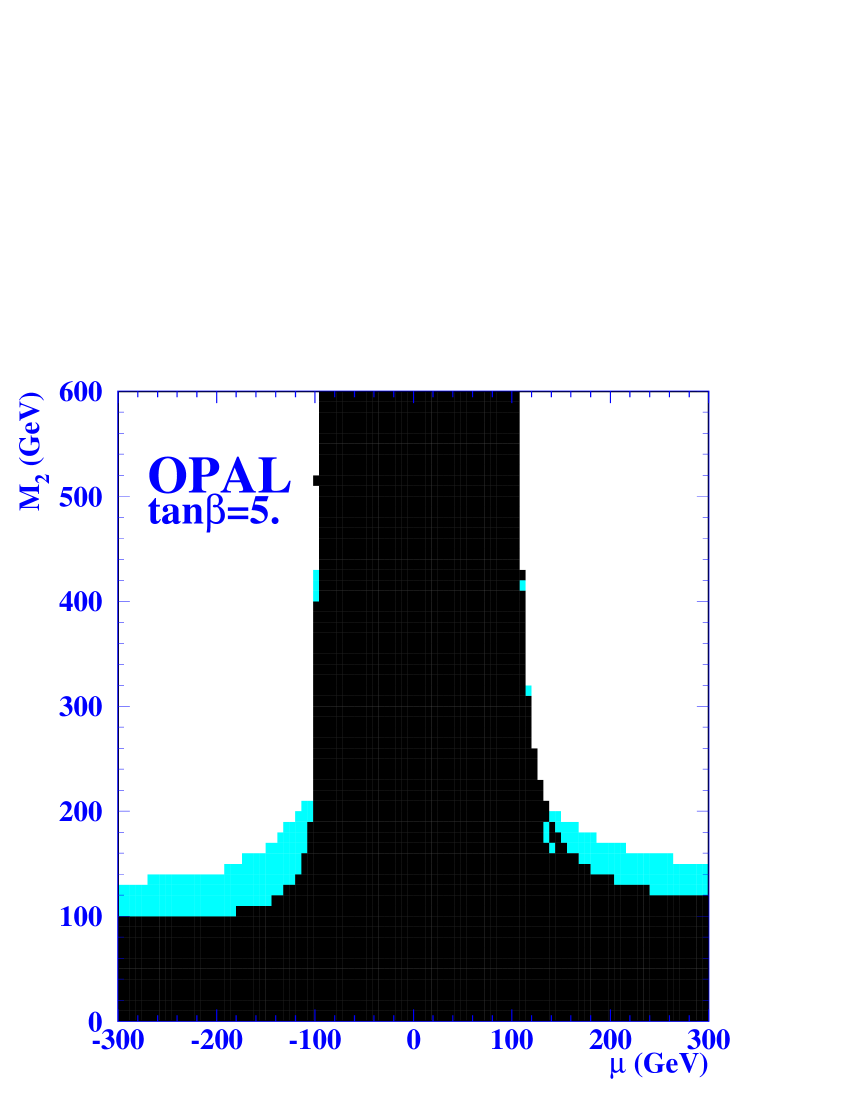
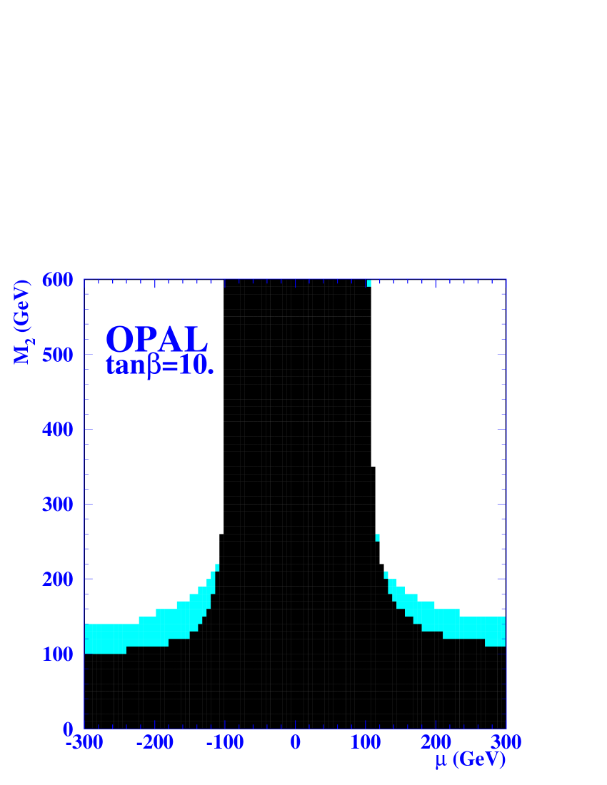
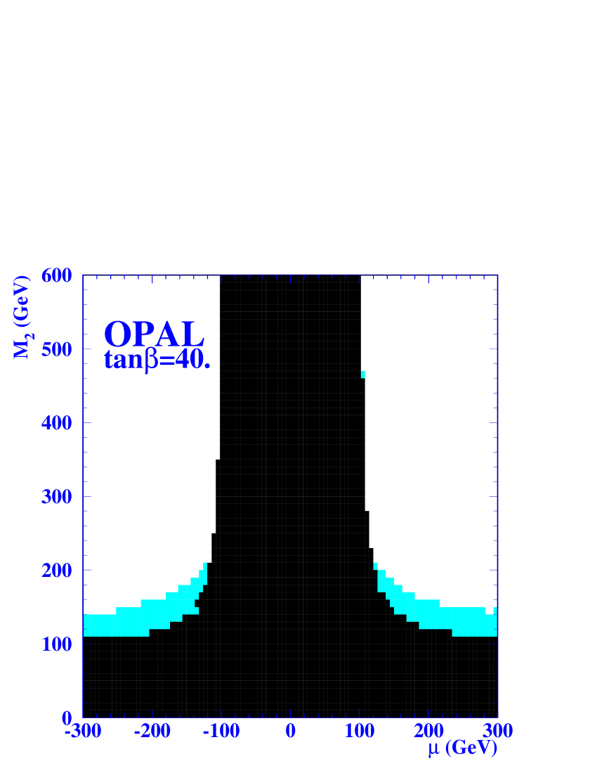
Figure 11: Regions of the CMSSM parameter space excluded by the OPAL search are shown in black. These include regions excluded by the OPAL data taken at energies up to 189 GeV [5] as well as those excluded with the present dataset and analysis. The regions with the lighter shading are kinematically accessible for either $\tilde{\chi}^{+}_{1}\tilde{\chi}^{-}_{1}$ or $\tilde{\chi}^{0}_{2}\tilde{\chi}^{0}_{1}$ production at $\sqrt{s}=208$ GeV, but are not excluded. These results are valid for $m_{0}\geq 500$ GeV and $A_{0}=0$ and for the values of $\tan\beta$ indicated on the individual plots.

The final step is to see what masses of charginos and neutralinos are excluded in the CMSSM. The kinematically accessible regions of the $M_{\tilde{\chi}^{\pm}_{1}},M_{\tilde{\chi}^{0}_{1}}$ and $M_{\tilde{\chi}^{0}_{2}},M_{\tilde{\chi}^{0}_{1}}$ planes are divided into a 1 by 1 GeV grid. All of the scanned $(M_{2},\mu,\tan\beta)$ points are examined to see what masses they predict for the lightest chargino and two lightest neutralinos. The smallest cross-section predicted in any 1 by 1 GeV grid square is compared with the cross-section limit. The CMSSM exclusions for the chargino mass plane are shown for the five values of $\tan\beta$ in figure 12 and the neutralino mass plane exclusions are shown in figure 13.

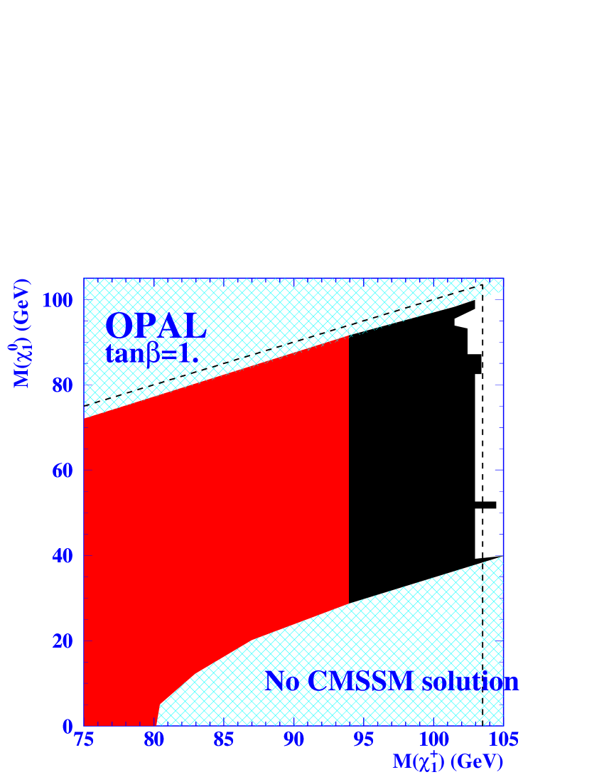
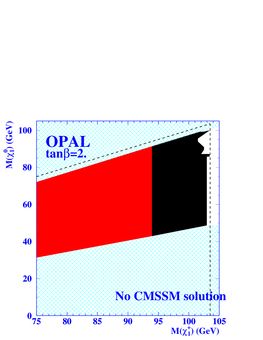
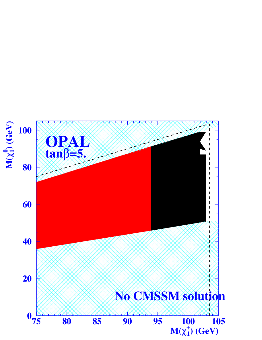
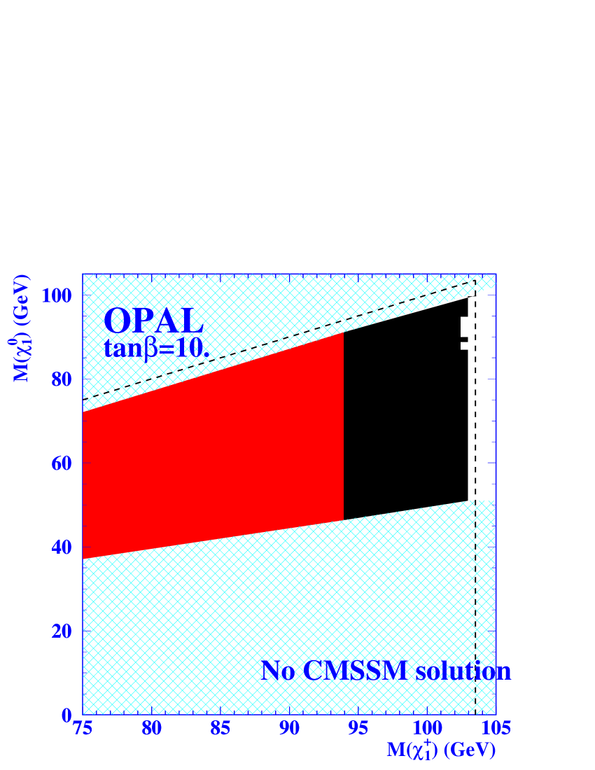
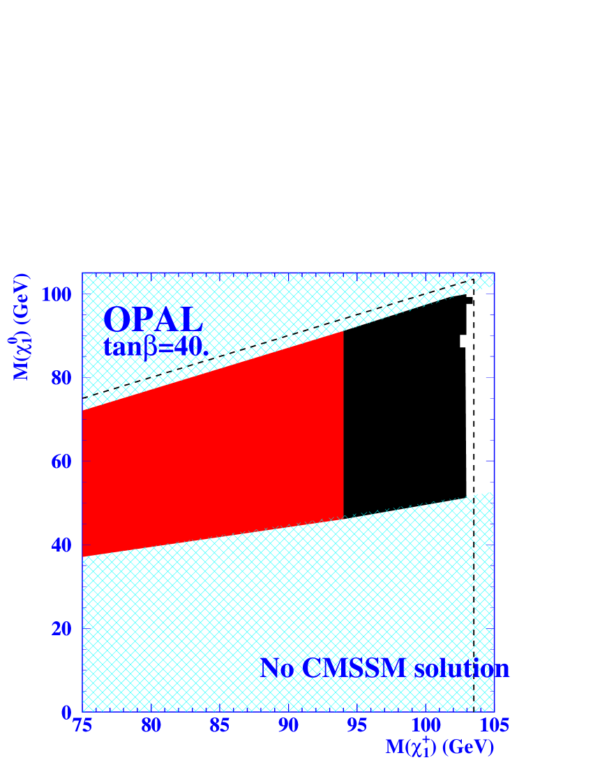
Figure 12: The shaded regions of the $\tilde{\chi}^{\pm}_{1}-\tilde{\chi}^{0}_{1}$ mass plane are excluded by OPAL data, with the lighter colour showing the region excluded by previously published searches [5] at centre-of-mass energies up to 189 GeV, and the black region being excluded by the present search. The kinematic limits of the chargino search are indicated by dotted lines; the very small excluded regions outside these limits are due to the neutralino search. The cross-hatched regions labelled “No CMSSM solution” correspond to regions of the parameter space having no solution in the CMSSM. The regions left white are not excluded.

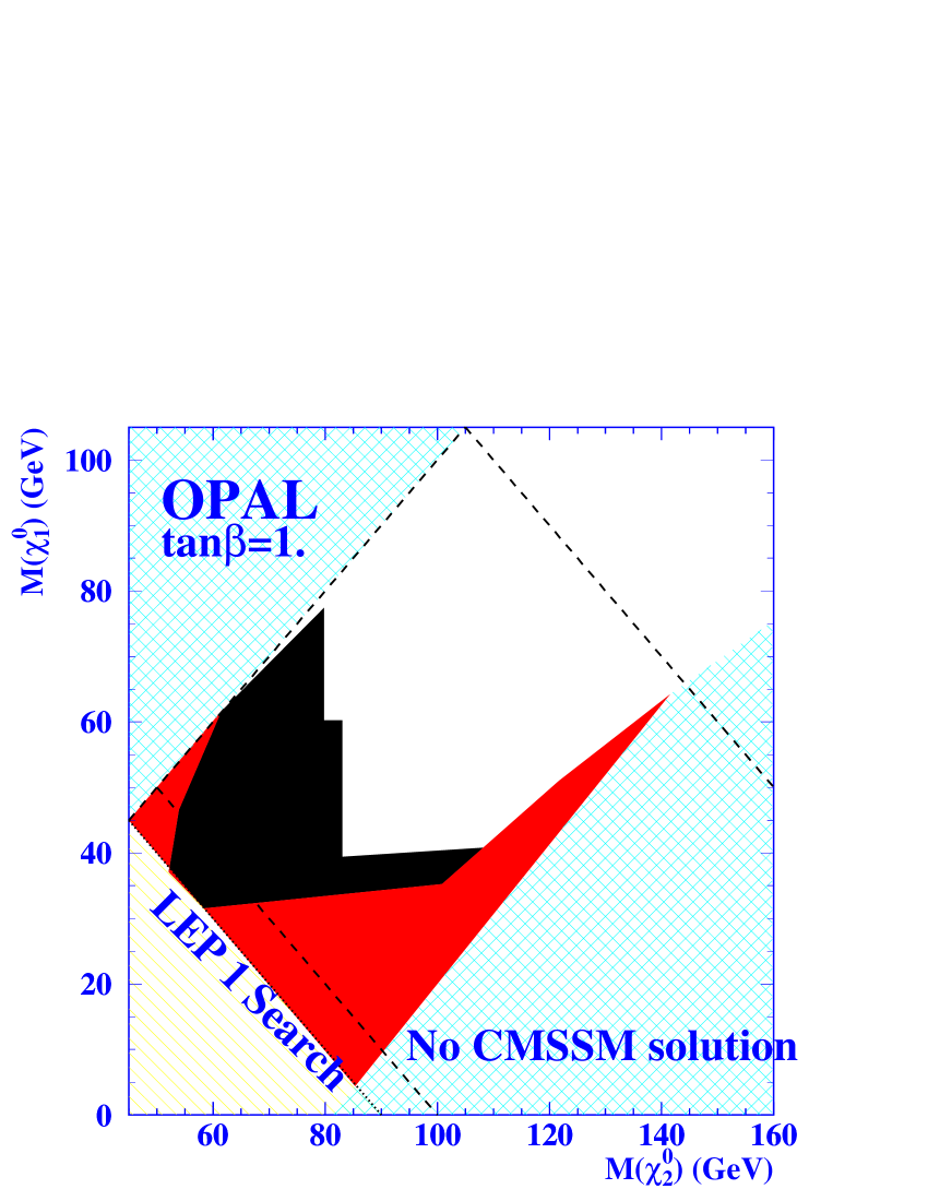
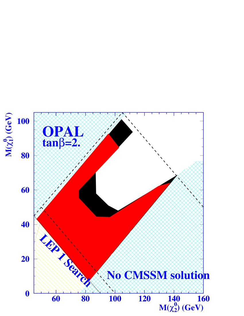
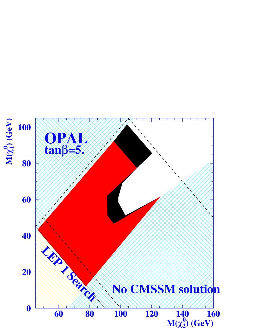
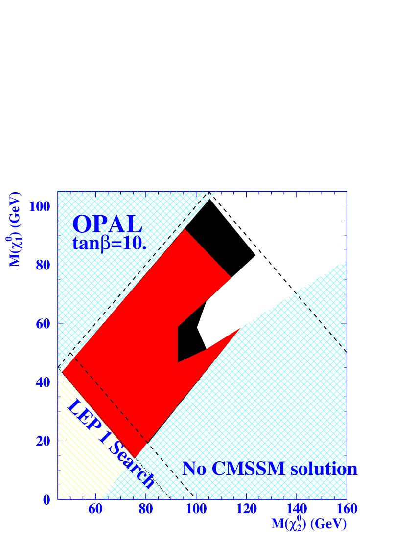
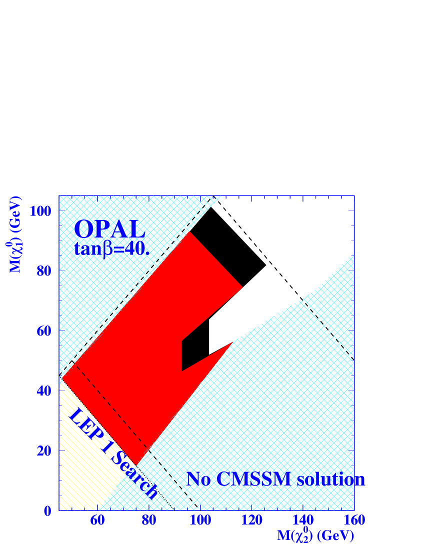
Figure 13: The shaded regions of the $\tilde{\chi}^{0}_{2}-\tilde{\chi}^{0}_{1}$ mass plane are excluded by OPAL data, with the lighter colour showing the region excluded by previously published searches [5] at centre-of-mass energies up to 189 GeV, and the black region being excluded by the present search. The kinematic limits of the neutralino search are indicated by dashed lines. The dashed line at $M_{\tilde{\chi}^{0}_{2}}+M_{\tilde{\chi}^{0}_{1}}=100$ GeV is simply a reminder that for the present analysis, no $\tilde{\chi}^{0}_{2}\tilde{\chi}^{0}_{1}$ Monte Carlo events were generated with lower masses; exclusion shown in black below this line is purely due to the chargino searches. The singly hatched region labelled “LEP 1 Search” is the region kinematically accessible to LEP 1 searches; it was not considered in this study. The cross-hatched region labelled “No CMSSM solution” corresponds to regions of the parameter space having no solution in the CMSSM. The regions left white cannot be excluded by the data.

Assuming that $m_{0}\geq 500$ GeV and $A_{0}=0$, the following conclusions can be made. For $\Delta M>5$ GeV, charginos with masses less than 101 GeV are excluded for all $\tan\beta$. For $\Delta M>5$ GeV, $\tilde{\chi}^{0}_{2}$ with masses less than 78 GeV and $\tilde{\chi}^{0}_{1}$ with masses less than 40 GeV are excluded for all $\tan\beta$.

8 Conclusions

No hint of charginos or neutralinos was observed in the data from OPAL. The cross-section limits presented in this paper for charginos or neutralinos decaying to particular final states may be regarded as completely model-independent and can be used to set limits on any model. Limits are set on the cross-section for chargino pair production by combining the three chargino final states under the assumption that all charginos decay to a virtual $\mathrm{W}$, which then decays with the usual branching ratios to leptons and hadrons. Limits are calculated for the specific example of the Constrained MSSM in the absence of light sfermions or mixing between right- and left-handed sfermions. Charginos are excluded almost up to the kinematic limit set by the maximum LEP beam energy of about 104 GeV.

References

-
[1]
H.P. Nilles, Phys. Rep. 110 (1984) 1;
H.E. Haber and G.L. Kane, Phys. Rep. 117 (1985) 75. - [2] J.L. Feng and M.J. Strassler, Phys. Rev. D51 (1995) 4661.
- [3] S. Ambrosanio and B. Mele, Phys. Rev. D52 (1995) 3900.
- [4] The OPAL Collaboration, G. Abbiendi et al., ‘Search for Anomalous Production of Di-lepton Events with Missing Transverse Momentum in Collisions at 183–209 GeV’, 10th July 2003, CERN-EP-2003-040, Accepted by Eur. Phys J. C.
- [5] G. Abbiendi et al., Eur. Phys. J. C14 (2000) 187.
- [6] G. Abbiendi et al., Eur. Phys. J. C8 (1999) 255.
- [7] K. Ackerstaff et al., Eur. Phys. J. C2 (1998) 213.
- [8] G. Abbiendi et al., Eur. Phys. J C14 (2000) 51.
- [9] OPAL Collab., K. Ahmet et al., Nucl. Instr. Meth. A305 (1991) 275.
- [10] S. Anderson et al., Nucl. Instr. Meth. A403 (1998) 326.
- [11] G. Aguillion et al., Nucl. Instr. Meth. A417 (1998) 266.
- [12] B.E. Anderson et al., IEEE Trans. on Nucl. Science 41 (1994) 845.
- [13] C. Dionisi et al., in ‘Physics at LEP2’, eds. G. Altarelli, T. Sjöstrand and F. Zwirner, CERN 96-01, vol.2, 337.
-
[14]
T. Sjöstrand, Comp. Phys. Comm. 82 (1994) 74;
T. Sjöstrand, Lund University report LU TP 95-20. - [15] G. Montagna et al., Nucl. Phys. B541 (1999) 31.
- [16] S. Jadach, W. Płaczek and B.F.L. Ward, Phys. Lett B390 (1997) 298.
- [17] D. Karlen, Nucl. Phys. B289 (1987) 23.
-
[18]
S. Jadach, B.F.L. Ward and Z. Wa̧s, Comp. Phys. Comm.130 (2000) 260;
S. Jadach, B.F.L. Ward and Z. Wa̧s, Phys. Lett. B449 (1999) 97. - [19] F.A. Berends, R. Kleiss, Nucl. Phys. B186 (1981) 22.
- [20] S. Jadach, W. Płaczek, M. Skrzypek, B.F.L. Ward and Z. Wa̧s, Comp. Phys. Comm.119 (1999) 272.
- [21] J. Fujimoto et al., Comp. Phys. Comm. 100 (1997) 128.
- [22] J.A.M. Vermaseren, Nucl. Phys. B229 (1983) 347.
-
[23]
F.A. Berends, P.H. Daverveldt and R. Kleiss, Nucl.Phys B253
(1985) 421;
F.A. Berends, P.H. Daverveldt and R. Kleiss, Comput. Phys. Comm. 40 (1986) 271;
F.A. Berends, P.H. Daverveldt and R. Kleiss, Comput. Phys. Comm. 40 (1986) 285;
F.A. Berends, P.H. Daverveldt and R. Kleiss, Comput. Phys. Comm. 40 (1986) 309. -
[24]
R. Engel, Z. Phys. C66 (1995) 203;
R. Engel and J. Ranft, Phys. Rev. D54 (1996) 4246. -
[25]
T. Sjöstrand, Comp. Phys. Comm. 82 (1994) 74.
T. Sjöstrand, Lund University report LU TP 95-20. - [26] G. Marchesini et al., Comp. Phys. Comm. 67 (1992) 465.
- [27] J. Allison et al., Nucl. Instr. Meth. A317 (1992) 47.
- [28] D. Karlen, Comp. in. Physics, 12 (1998) 380.
- [29] D. Futyan, “Search for Supersymmetry Using Acoplanar Lepton Pair Events at OPAL”, Appendix, PhD. thesis, Univerity of Manchester, December 1999. http://hepwww.ph.man.ac.uk/theses/DavidFutyan.ps.
- [30] T.E. Marchant, “Search for New Physics Using Acoplanar Lepton Pair Events in Collisions at 183-208 GeV”, Chapter 5, PhD. thesis, University of Manchester, March 2002. http://hepwww.ph.man.ac.uk/theses/TomMarchant.ps.
- [31] S. Catani et al., Phys. Lett. B269 (1991) 432.
- [32] K. Ackerstaff et al., Eur. Phys. J. C1 (1998) 395.
- [33] N.Ghodbane, S.Katsanevas, P.Morawitz, E.Perez, SUSYGEN 3, hep-ph/9909499.