CERN–EP/2003-065

28 Mai 2003

DELPHI Collaboration

Abstract

Final results from the DELPHI Collaboration on the lifetime of ${\mathrm{B}^{+}}$ and ${\mathrm{B}^{0}}$ mesons and the mean b-hadron lifetime, are presented using the data collected at the ${\mathrm{Z}}^{0}$ peak in 1994 and 1995. Elaborate, inclusive, secondary vertexing methods have been employed to ensure a b-hadron reconstruction with good efficiency. To separate samples of ${\mathrm{B}^{+}}$ and ${\mathrm{B}^{0}}$ mesons, high performance neural network techniques are used that achieve very high purity signals. The results obtained are:

$\tau_{{\mathrm{B}}^{+}}$	=	1.624	$\pm 0.014$ (stat)	$\pm 0.018$ (syst) ps
$\tau_{{\mathrm{B}}^{0}}$	=	1.531	$\pm 0.021$ (stat)	$\pm 0.031$ (syst) ps
$\frac{\tau_{{\mathrm{B}}^{+}}}{\tau_{{\mathrm{B}}^{0}}}$	=	1.060	$\pm 0.021$ (stat)	$\pm 0.024$ (syst)

and for the average b-hadron lifetime:

$\tau_{{\mathrm{b}}}$

=

1.570

$\pm 0.005$ (stat)

$\pm 0.008$ (syst) ps.

(Accepted by Eur. Phys. J.)

J.Abdallah${}^{\ref{LPNHE}}$, P.Abreu${}^{\ref{LIP}}$, W.Adam${}^{\ref{VIENNA}}$, P.Adzic${}^{\ref{DEMOKRITOS}}$, T.Albrecht${}^{\ref{KARLSRUHE}}$, T.Alderweireld${}^{\ref{AIM}}$, R.Alemany-Fernandez${}^{\ref{CERN}}$, T.Allmendinger${}^{\ref{KARLSRUHE}}$, P.P.Allport${}^{\ref{LIVERPOOL}}$, U.Amaldi${}^{\ref{MILANO2}}$, N.Amapane${}^{\ref{TORINO}}$, S.Amato${}^{\ref{UFRJ}}$, E.Anashkin${}^{\ref{PADOVA}}$, A.Andreazza${}^{\ref{MILANO}}$, S.Andringa${}^{\ref{LIP}}$, N.Anjos${}^{\ref{LIP}}$, P.Antilogus${}^{\ref{LYON}}$, W-D.Apel${}^{\ref{KARLSRUHE}}$, Y.Arnoud${}^{\ref{GRENOBLE}}$, S.Ask${}^{\ref{LUND}}$, B.Asman${}^{\ref{STOCKHOLM}}$, J.E.Augustin${}^{\ref{LPNHE}}$, A.Augustinus${}^{\ref{CERN}}$, P.Baillon${}^{\ref{CERN}}$, A.Ballestrero${}^{\ref{TORINOTH}}$, P.Bambade${}^{\ref{LAL}}$, R.Barbier${}^{\ref{LYON}}$, D.Bardin${}^{\ref{JINR}}$, G.J.Barker${}^{\ref{KARLSRUHE}}$, A.Baroncelli${}^{\ref{ROMA3}}$, M.Battaglia${}^{\ref{CERN}}$, M.Baubillier${}^{\ref{LPNHE}}$, K-H.Becks${}^{\ref{WUPPERTAL}}$, M.Begalli${}^{\ref{BRASIL}}$, A.Behrmann${}^{\ref{WUPPERTAL}}$, E.Ben-Haim${}^{\ref{LAL}}$, N.Benekos${}^{\ref{NTU-ATHENS}}$, A.Benvenuti${}^{\ref{BOLOGNA}}$, C.Berat${}^{\ref{GRENOBLE}}$, M.Berggren${}^{\ref{LPNHE}}$, L.Berntzon${}^{\ref{STOCKHOLM}}$, D.Bertrand${}^{\ref{AIM}}$, M.Besancon${}^{\ref{SACLAY}}$, N.Besson${}^{\ref{SACLAY}}$, D.Bloch${}^{\ref{CRN}}$, M.Blom${}^{\ref{NIKHEF}}$, M.Bluj${}^{\ref{WARSZAWA}}$, M.Bonesini${}^{\ref{MILANO2}}$, M.Boonekamp${}^{\ref{SACLAY}}$, P.S.L.Booth${}^{\ref{LIVERPOOL}}$, G.Borisov${}^{\ref{LANCASTER}}$, O.Botner${}^{\ref{UPPSALA}}$, B.Bouquet${}^{\ref{LAL}}$, T.J.V.Bowcock${}^{\ref{LIVERPOOL}}$, I.Boyko${}^{\ref{JINR}}$, M.Bracko${}^{\ref{SLOVENIJA}}$, R.Brenner${}^{\ref{UPPSALA}}$, E.Brodet${}^{\ref{OXFORD}}$, P.Bruckman${}^{\ref{KRAKOW1}}$, J.M.Brunet${}^{\ref{CDF}}$, L.Bugge${}^{\ref{OSLO}}$, P.Buschmann${}^{\ref{WUPPERTAL}}$, M.Calvi${}^{\ref{MILANO2}}$, T.Camporesi${}^{\ref{CERN}}$, V.Canale${}^{\ref{ROMA2}}$, F.Carena${}^{\ref{CERN}}$, N.Castro${}^{\ref{LIP}}$, F.Cavallo${}^{\ref{BOLOGNA}}$, M.Chapkin${}^{\ref{SERPUKHOV}}$, Ph.Charpentier${}^{\ref{CERN}}$, P.Checchia${}^{\ref{PADOVA}}$, R.Chierici${}^{\ref{CERN}}$, P.Chliapnikov${}^{\ref{SERPUKHOV}}$, J.Chudoba${}^{\ref{CERN}}$, S.U.Chung${}^{\ref{CERN}}$, K.Cieslik${}^{\ref{KRAKOW1}}$, P.Collins${}^{\ref{CERN}}$, R.Contri${}^{\ref{GENOVA}}$, G.Cosme${}^{\ref{LAL}}$, F.Cossutti${}^{\ref{TU}}$, M.J.Costa${}^{\ref{VALENCIA}}$, B.Crawley${}^{\ref{AMES}}$, D.Crennell${}^{\ref{RAL}}$, J.Cuevas${}^{\ref{OVIEDO}}$, J.D’Hondt${}^{\ref{AIM}}$, J.Dalmau${}^{\ref{STOCKHOLM}}$, T.da Silva${}^{\ref{UFRJ}}$, W.Da Silva${}^{\ref{LPNHE}}$, G.Della Ricca${}^{\ref{TU}}$, A.De Angelis${}^{\ref{TU}}$, W.De Boer${}^{\ref{KARLSRUHE}}$, C.De Clercq${}^{\ref{AIM}}$, B.De Lotto${}^{\ref{TU}}$, N.De Maria${}^{\ref{TORINO}}$, A.De Min${}^{\ref{PADOVA}}$, L.de Paula${}^{\ref{UFRJ}}$, L.Di Ciaccio${}^{\ref{ROMA2}}$, A.Di Simone${}^{\ref{ROMA3}}$, K.Doroba${}^{\ref{WARSZAWA}}$, J.Drees${}^{\ref{WUPPERTAL},\ref{CERN}}$, M.Dris${}^{\ref{NTU-ATHENS}}$, G.Eigen${}^{\ref{BERGEN}}$, T.Ekelof${}^{\ref{UPPSALA}}$, M.Ellert${}^{\ref{UPPSALA}}$, M.Elsing${}^{\ref{CERN}}$, M.C.Espirito Santo${}^{\ref{LIP}}$, G.Fanourakis${}^{\ref{DEMOKRITOS}}$, D.Fassouliotis${}^{\ref{DEMOKRITOS},\ref{ATHENS}}$, M.Feindt${}^{\ref{KARLSRUHE}}$, J.Fernandez${}^{\ref{SANTANDER}}$, A.Ferrer${}^{\ref{VALENCIA}}$, F.Ferro${}^{\ref{GENOVA}}$, U.Flagmeyer${}^{\ref{WUPPERTAL}}$, H.Foeth${}^{\ref{CERN}}$, E.Fokitis${}^{\ref{NTU-ATHENS}}$, F.Fulda-Quenzer${}^{\ref{LAL}}$, J.Fuster${}^{\ref{VALENCIA}}$, M.Gandelman${}^{\ref{UFRJ}}$, C.Garcia${}^{\ref{VALENCIA}}$, Ph.Gavillet${}^{\ref{CERN}}$, E.Gazis${}^{\ref{NTU-ATHENS}}$, R.Gokieli${}^{\ref{CERN},\ref{WARSZAWA}}$, B.Golob${}^{\ref{SLOVENIJA}}$, G.Gomez-Ceballos${}^{\ref{SANTANDER}}$, P.Goncalves${}^{\ref{LIP}}$, E.Graziani${}^{\ref{ROMA3}}$, G.Grosdidier${}^{\ref{LAL}}$, K.Grzelak${}^{\ref{WARSZAWA}}$, J.Guy${}^{\ref{RAL}}$, C.Haag${}^{\ref{KARLSRUHE}}$, A.Hallgren${}^{\ref{UPPSALA}}$, K.Hamacher${}^{\ref{WUPPERTAL}}$, K.Hamilton${}^{\ref{OXFORD}}$, J.Hansen${}^{\ref{OSLO}}$, S.Haug${}^{\ref{OSLO}}$, F.Hauler${}^{\ref{KARLSRUHE}}$, V.Hedberg${}^{\ref{LUND}}$, M.Hennecke${}^{\ref{KARLSRUHE}}$, H.Herr${}^{\ref{CERN}}$, J.Hoffman${}^{\ref{WARSZAWA}}$, S-O.Holmgren${}^{\ref{STOCKHOLM}}$, P.J.Holt${}^{\ref{CERN}}$, M.A.Houlden${}^{\ref{LIVERPOOL}}$, K.Hultqvist${}^{\ref{STOCKHOLM}}$, J.N.Jackson${}^{\ref{LIVERPOOL}}$, G.Jarlskog${}^{\ref{LUND}}$, P.Jarry${}^{\ref{SACLAY}}$, D.Jeans${}^{\ref{OXFORD}}$, E.K.Johansson${}^{\ref{STOCKHOLM}}$, P.D.Johansson${}^{\ref{STOCKHOLM}}$, P.Jonsson${}^{\ref{LYON}}$, C.Joram${}^{\ref{CERN}}$, L.Jungermann${}^{\ref{KARLSRUHE}}$, F.Kapusta${}^{\ref{LPNHE}}$, S.Katsanevas${}^{\ref{LYON}}$, E.Katsoufis${}^{\ref{NTU-ATHENS}}$, G.Kernel${}^{\ref{SLOVENIJA}}$, B.P.Kersevan${}^{\ref{CERN},\ref{SLOVENIJA}}$, A.Kiiskinen${}^{\ref{HELSINKI}}$, B.T.King${}^{\ref{LIVERPOOL}}$, N.J.Kjaer${}^{\ref{CERN}}$, P.Kluit${}^{\ref{NIKHEF}}$, P.Kokkinias${}^{\ref{DEMOKRITOS}}$, C.Kourkoumelis${}^{\ref{ATHENS}}$, O.Kouznetsov${}^{\ref{JINR}}$, Z.Krumstein${}^{\ref{JINR}}$, M.Kucharczyk${}^{\ref{KRAKOW1}}$, J.Lamsa${}^{\ref{AMES}}$, G.Leder${}^{\ref{VIENNA}}$, F.Ledroit${}^{\ref{GRENOBLE}}$, L.Leinonen${}^{\ref{STOCKHOLM}}$, R.Leitner${}^{\ref{NC}}$, J.Lemonne${}^{\ref{AIM}}$, V.Lepeltier${}^{\ref{LAL}}$, T.Lesiak${}^{\ref{KRAKOW1}}$, W.Liebig${}^{\ref{WUPPERTAL}}$, D.Liko${}^{\ref{VIENNA}}$, A.Lipniacka${}^{\ref{STOCKHOLM}}$, J.H.Lopes${}^{\ref{UFRJ}}$, J.M.Lopez${}^{\ref{OVIEDO}}$, D.Loukas${}^{\ref{DEMOKRITOS}}$, P.Lutz${}^{\ref{SACLAY}}$, L.Lyons${}^{\ref{OXFORD}}$, J.MacNaughton${}^{\ref{VIENNA}}$, A.Malek${}^{\ref{WUPPERTAL}}$, S.Maltezos${}^{\ref{NTU-ATHENS}}$, F.Mandl${}^{\ref{VIENNA}}$, J.Marco${}^{\ref{SANTANDER}}$, R.Marco${}^{\ref{SANTANDER}}$, B.Marechal${}^{\ref{UFRJ}}$, M.Margoni${}^{\ref{PADOVA}}$, J-C.Marin${}^{\ref{CERN}}$, C.Mariotti${}^{\ref{CERN}}$, A.Markou${}^{\ref{DEMOKRITOS}}$, C.Martinez-Rivero${}^{\ref{SANTANDER}}$, J.Masik${}^{\ref{FZU}}$, N.Mastroyiannopoulos${}^{\ref{DEMOKRITOS}}$, F.Matorras${}^{\ref{SANTANDER}}$, C.Matteuzzi${}^{\ref{MILANO2}}$, F.Mazzucato${}^{\ref{PADOVA}}$, M.Mazzucato${}^{\ref{PADOVA}}$, R.Mc Nulty${}^{\ref{LIVERPOOL}}$, C.Meroni${}^{\ref{MILANO}}$, W.T.Meyer${}^{\ref{AMES}}$, E.Migliore${}^{\ref{TORINO}}$, W.Mitaroff${}^{\ref{VIENNA}}$, U.Mjoernmark${}^{\ref{LUND}}$, T.Moa${}^{\ref{STOCKHOLM}}$, M.Moch${}^{\ref{KARLSRUHE}}$, K.Moenig${}^{\ref{CERN},\ref{DESY}}$, R.Monge${}^{\ref{GENOVA}}$, J.Montenegro${}^{\ref{NIKHEF}}$, D.Moraes${}^{\ref{UFRJ}}$, S.Moreno${}^{\ref{LIP}}$, P.Morettini${}^{\ref{GENOVA}}$, U.Mueller${}^{\ref{WUPPERTAL}}$, K.Muenich${}^{\ref{WUPPERTAL}}$, M.Mulders${}^{\ref{NIKHEF}}$, L.Mundim${}^{\ref{BRASIL}}$, W.Murray${}^{\ref{RAL}}$, B.Muryn${}^{\ref{KRAKOW2}}$, G.Myatt${}^{\ref{OXFORD}}$, T.Myklebust${}^{\ref{OSLO}}$, M.Nassiakou${}^{\ref{DEMOKRITOS}}$, F.Navarria${}^{\ref{BOLOGNA}}$, K.Nawrocki${}^{\ref{WARSZAWA}}$, R.Nicolaidou${}^{\ref{SACLAY}}$, M.Nikolenko${}^{\ref{JINR},\ref{CRN}}$, A.Oblakowska-Mucha${}^{\ref{KRAKOW2}}$, V.Obraztsov${}^{\ref{SERPUKHOV}}$, A.Olshevski${}^{\ref{JINR}}$, A.Onofre${}^{\ref{LIP}}$, R.Orava${}^{\ref{HELSINKI}}$, K.Osterberg${}^{\ref{HELSINKI}}$, A.Ouraou${}^{\ref{SACLAY}}$, A.Oyanguren${}^{\ref{VALENCIA}}$, M.Paganoni${}^{\ref{MILANO2}}$, S.Paiano${}^{\ref{BOLOGNA}}$, J.P.Palacios${}^{\ref{LIVERPOOL}}$, H.Palka${}^{\ref{KRAKOW1}}$, Th.D.Papadopoulou${}^{\ref{NTU-ATHENS}}$, L.Pape${}^{\ref{CERN}}$, C.Parkes${}^{\ref{GLASGOW}}$, F.Parodi${}^{\ref{GENOVA}}$, U.Parzefall${}^{\ref{CERN}}$, A.Passeri${}^{\ref{ROMA3}}$, O.Passon${}^{\ref{WUPPERTAL}}$, L.Peralta${}^{\ref{LIP}}$, V.Perepelitsa${}^{\ref{VALENCIA}}$, A.Perrotta${}^{\ref{BOLOGNA}}$, A.Petrolini${}^{\ref{GENOVA}}$, J.Piedra${}^{\ref{SANTANDER}}$, L.Pieri${}^{\ref{ROMA3}}$, F.Pierre${}^{\ref{SACLAY}}$, M.Pimenta${}^{\ref{LIP}}$, E.Piotto${}^{\ref{CERN}}$, T.Podobnik${}^{\ref{SLOVENIJA}}$, V.Poireau${}^{\ref{CERN}}$, M.E.Pol${}^{\ref{BRASIL}}$, G.Polok${}^{\ref{KRAKOW1}}$, P.Poropat^†${}^{\ref{TU}}$, V.Pozdniakov${}^{\ref{JINR}}$, N.Pukhaeva${}^{\ref{AIM},\ref{JINR}}$, A.Pullia${}^{\ref{MILANO2}}$, J.Rames${}^{\ref{FZU}}$, L.Ramler${}^{\ref{KARLSRUHE}}$, A.Read${}^{\ref{OSLO}}$, P.Rebecchi${}^{\ref{CERN}}$, J.Rehn${}^{\ref{KARLSRUHE}}$, D.Reid${}^{\ref{NIKHEF}}$, R.Reinhardt${}^{\ref{WUPPERTAL}}$, P.Renton${}^{\ref{OXFORD}}$, F.Richard${}^{\ref{LAL}}$, J.Ridky${}^{\ref{FZU}}$, M.Rivero${}^{\ref{SANTANDER}}$, D.Rodriguez${}^{\ref{SANTANDER}}$, A.Romero${}^{\ref{TORINO}}$, P.Ronchese${}^{\ref{PADOVA}}$, E.Rosenberg${}^{\ref{AMES}}$, P.Roudeau${}^{\ref{LAL}}$, T.Rovelli${}^{\ref{BOLOGNA}}$, V.Ruhlmann-Kleider${}^{\ref{SACLAY}}$, D.Ryabtchikov${}^{\ref{SERPUKHOV}}$, A.Sadovsky${}^{\ref{JINR}}$, L.Salmi${}^{\ref{HELSINKI}}$, J.Salt${}^{\ref{VALENCIA}}$, A.Savoy-Navarro${}^{\ref{LPNHE}}$, U.Schwickerath${}^{\ref{CERN}}$, A.Segar${}^{\ref{OXFORD}}$, R.Sekulin${}^{\ref{RAL}}$, M.Siebel${}^{\ref{WUPPERTAL}}$, A.Sisakian${}^{\ref{JINR}}$, G.Smadja${}^{\ref{LYON}}$, O.Smirnova${}^{\ref{LUND}}$, A.Sokolov${}^{\ref{SERPUKHOV}}$, A.Sopczak${}^{\ref{LANCASTER}}$, R.Sosnowski${}^{\ref{WARSZAWA}}$, T.Spassov${}^{\ref{CERN}}$, M.Stanitzki${}^{\ref{KARLSRUHE}}$, A.Stocchi${}^{\ref{LAL}}$, J.Strauss${}^{\ref{VIENNA}}$, B.Stugu${}^{\ref{BERGEN}}$, M.Szczekowski${}^{\ref{WARSZAWA}}$, M.Szeptycka${}^{\ref{WARSZAWA}}$, T.Szumlak${}^{\ref{KRAKOW2}}$, T.Tabarelli${}^{\ref{MILANO2}}$, A.C.Taffard${}^{\ref{LIVERPOOL}}$, F.Tegenfeldt${}^{\ref{UPPSALA}}$, J.Timmermans${}^{\ref{NIKHEF}}$, L.Tkatchev${}^{\ref{JINR}}$, M.Tobin${}^{\ref{LIVERPOOL}}$, S.Todorovova${}^{\ref{FZU}}$, B.Tome${}^{\ref{LIP}}$, A.Tonazzo${}^{\ref{MILANO2}}$, P.Tortosa${}^{\ref{VALENCIA}}$, P.Travnicek${}^{\ref{FZU}}$, D.Treille${}^{\ref{CERN}}$, G.Tristram${}^{\ref{CDF}}$, M.Trochimczuk${}^{\ref{WARSZAWA}}$, C.Troncon${}^{\ref{MILANO}}$, M-L.Turluer${}^{\ref{SACLAY}}$, I.A.Tyapkin${}^{\ref{JINR}}$, P.Tyapkin${}^{\ref{JINR}}$, S.Tzamarias${}^{\ref{DEMOKRITOS}}$, V.Uvarov${}^{\ref{SERPUKHOV}}$, G.Valenti${}^{\ref{BOLOGNA}}$, P.Van Dam${}^{\ref{NIKHEF}}$, J.Van Eldik${}^{\ref{CERN}}$, A.Van Lysebetten${}^{\ref{AIM}}$, N.van Remortel${}^{\ref{AIM}}$, I.Van Vulpen${}^{\ref{CERN}}$, G.Vegni${}^{\ref{MILANO}}$, F.Veloso${}^{\ref{LIP}}$, W.Venus${}^{\ref{RAL}}$, F.Verbeure${}^{\ref{AIM}}$, P.Verdier${}^{\ref{LYON}}$, V.Verzi${}^{\ref{ROMA2}}$, D.Vilanova${}^{\ref{SACLAY}}$, L.Vitale${}^{\ref{TU}}$, V.Vrba${}^{\ref{FZU}}$, H.Wahlen${}^{\ref{WUPPERTAL}}$, A.J.Washbrook${}^{\ref{LIVERPOOL}}$, C.Weiser${}^{\ref{KARLSRUHE}}$, D.Wicke${}^{\ref{CERN}}$, J.Wickens${}^{\ref{AIM}}$, G.Wilkinson${}^{\ref{OXFORD}}$, M.Winter${}^{\ref{CRN}}$, M.Witek${}^{\ref{KRAKOW1}}$, O.Yushchenko${}^{\ref{SERPUKHOV}}$, A.Zalewska${}^{\ref{KRAKOW1}}$, P.Zalewski${}^{\ref{WARSZAWA}}$, D.Zavrtanik${}^{\ref{SLOVENIJA}}$, V.Zhuravlov${}^{\ref{JINR}}$, N.I.Zimin${}^{\ref{JINR}}$, A.Zintchenko${}^{\ref{JINR}}$, M.Zupan${}^{\ref{DEMOKRITOS}}$

1 Motivation and Overview

In addition to testing models of b-hadron decay, knowledge of b-hadron lifetimes is of importance in the determination of other Standard Model quantities such as the CKM matrix element $V_{{\mathrm{c}b}}$ and in measurements of the time dependence of neutral b-meson oscillations.

The Spectator Model provides the simplest description of b-hadron decay. Here, the lifetime depends only on the weak decay of the b-quark with the other light-quark constituent(s) playing no role in the decay dynamics. This, in turn, leads to the prediction that all b-hadron species have the same lifetime. Non-spectator effects however such as quark interference, $\mathrm{W}$ exchange and weak annihilation can induce lifetime differences among the different b-hadron species. Models of b-hadron decay based on expansions in $1/m_{{\mathrm{b}}}$ predict that, $\tau({\mathrm{\Lambda}_{b}})<\tau({\mathrm{B}^{0}})\sim\tau({\mathrm{B}_{s}})<\tau({\mathrm{B}^{+}})$, and this lifetime hierarchy has already been confirmed by experiment. There is a growing consensus between models that a difference in lifetime of order 5% should exist between the ${\mathrm{B}^{+}}$ and ${\mathrm{B}^{0}}$ meson [1] and it is currently measured to be, $\frac{\tau_{{\mathrm{B}}^{+}}}{\tau_{{\mathrm{B}}^{0}}}=1.085\pm 0.017$ [2]. Clearly, more precise lifetime measurements of all b-hadron species are valuable in order to test developments in b-hadron decay theory.

This paper reports on the measurement of the ${\mathrm{B}^{+}}$ and ${\mathrm{B}^{0}}$ meson lifetimes from data taken with the DELPHI detector at LEP I, in sub-samples separately enriched in ${\mathrm{B}^{+}}$ and ${\mathrm{B}^{0}}$ mesons. In addition, a measurement of the mean b-hadron lifetime $\tau_{\mathrm{b}}$ (i.e. with ${\mathrm{\Lambda}_{b}},{\mathrm{B}^{0}},{\mathrm{B}_{s}},{\mathrm{B}^{+}}$ unseparated) is obtained, which is a quantity of importance for many b-physics analyses at LEP e.g. in the extraction of the CKM matrix element $\left|V_{{\mathrm{c}b}}\right|$.

The analysis proceeds by reconstructing the proper time of b-hadron candidates ($t=Lm_{0}/pc$ where $L,p$ and $m_{0}$ are the decay length, momentum and rest mass respectively) and fitting the $t$ distribution in simulation to the data distribution in a $\chi^{2}$–minimisation procedure. In the fit for the ${\mathrm{B}^{+}}$ and ${\mathrm{B}^{0}}$ lifetimes, the ${\mathrm{B}_{s}}$ and ${\mathrm{\Lambda}_{b}}$ lifetimes are set to their measured values whereas in the fit for $\tau_{\mathrm{b}}$, all B-species are assumed to have the same lifetime and $\tau_{\mathrm{b}}$ is the only free parameter in the fit. The approach used is highly inclusive and based on the DELPHI inclusive B-physics package, BSAURUS [3]. Aspects of BSAURUS directly related to the analysis are presented in a summarised form but the reference should be consulted for full details of the package.

After describing parts of the DELPHI detector essential for this measurement in Section 2, the data sets are described in Section 3 and relevant aspects of BSAURUS are highlighted in Section 4. Section 5 describes the reconstruction of the B-candidate proper time from measurements of decay length and momentum. Samples with a $\sim 70$% purity in ${\mathrm{B}^{+}}$ or ${\mathrm{B}^{0}}$ mesons were achieved by use of a sophisticated neural network approach which is described in Section 6. Section 7 shows the results of the lifetime fits and finally, systematic uncertainties on the measurements are dealt with in Section 8.

2 The DELPHI Detector

A complete overview of the DELPHI detector [4] and of its performance [5] have been given in detail elsewhere. This analysis depends crucially on precision charged particle tracking performed by the Vertex Detector (VD), the Inner Detector, the Time Projection Chamber (TPC) and the Outer Detector. A highly uniform magnetic field of 1.23 T parallel to the electron beam direction, was provided by the superconducting solenoid throughout the tracking volume. The momentum of charged particles was measured with a precision of $\sigma_{p}/p\leq 1.5\%$ in the polar angle region $40^{\circ}\leq\theta\leq 140$ and for $p<10$ GeV/$c$.

The VD was of particular importance for the reconstruction of the decay vertices of short-lived particles and consisted of three layers of silicon microstrip detectors, called the Closer, Inner and Outer layers, at radii of 6.3 cm, 9 cm and 11 cm from the beam line respectively. The VD was upgraded [6] in 1994 and 1995 with double-sided microstrip detectors in the Closer and Outer layers providing coordinates in both $r\phi$ and $rz$. For polar angles of $44^{\circ}\leq\theta\leq 136^{\circ}$, a track crosses all three silicon layers of the VD. The measured intrinsic resolution is about 8 $\mu{\mathrm{m}}$ for the $r\phi$ coordinate while for $rz$ it depends on the incident polar angle of the track and reaches about 9 $\mu{\mathrm{m}}$ for tracks perpendicular to the modules. For tracks with hits in all three $r\phi$ VD layers the impact parameter resolution was $\sigma_{r\phi}^{2}=([61/(p\,\sin^{3/2}\theta)]^{2}+20^{2})$ $\mu{\mathrm{m}}$² and for tracks with hits in both $rz$ layers and with $\theta\approx 90^{\circ}$, $\sigma_{rz}^{2}=([67/(p\,\sin^{5/2}\theta)]^{2}+33^{2})$ $\mu{\mathrm{m}}$². Before the start of data taking in 1995 the ID was replaced with a similar device but with a larger polar angle coverage in preparation for LEP 2 running. The impact of this change on the current analysis is relatively minor.

Calorimeters detected photons and neutral hadrons by the total absorption of their energy. The High-density Projection Chamber (HPC) provided electromagnetic calorimetry coverage in the polar angle region $46^{\circ}<\theta<134^{\circ}$ giving a relative precision on the measured energy $E$ of $\sigma_{E}/E=0.32/\sqrt{E}\oplus 0.043$ ($E$ in GeV). In addition, each HPC module is essentially a small TPC which can chart the spatial development of showers and so provide an angular resolution better than that of the detector granularity alone. For high energy photons the angular resolutions were $\pm 1.7$ mrad in the azimuthal angle $\phi$ and $\pm 1.0$ mrad in the polar angle $\theta$.

The Hadron Calorimeter was installed in the return yoke of the DELPHI solenoid and provided a relative precision on the measured energy of $\sigma_{E}/E=1.12/\sqrt{E}\oplus 0.21$ ($E$ in GeV).

Powerful particle identification (see Section 4.4) was possible by the combination of $dE/dx$ information from the TPC (and to a lesser extent from the VD) with information from the DELPHI Ring Imaging CHerenkov counters (RICH) in both the forward and barrel regions. The RICH devices utilised both liquid and gas radiators in order to optimise coverage across a wide momentum range: liquid was used for the momentum range from 0.7 GeV/$c$ to 8 GeV/$c$ and the gas radiator for the range 2.5 GeV/$c$ to 25 GeV/$c$.

3 Data Samples

3.1 Hadronic Event Selection

Hadronic ${\mathrm{Z}^{0}}$ decays were selected by the following requirements:

• at least 5 reconstructed charged particles,

• the summed energy of charged particles (with momentum $>0.2$ GeV/$c$) had to be larger than 12% of the centre-of-mass energy, with at least 3% of it in each of the forward and backward hemispheres defined with respect to the beam axis.

Due to the evolution of the DELPHI tracking detectors with time, and run-specific details such as the RICH efficiency, the data were treated throughout this analysis as two independent data sets for the periods 1994 and 1995. The hadronic event cuts selected approximately 1.4 million events in 1994 and 0.7 million events in 1995.

3.2 Event Selection

Hadronic events were enhanced in ${\mathrm{Z}}^{0}\rightarrow{\mathrm{b}}\bar{{\mathrm{b}}}$ events, by cutting on the DELPHI combined b-tagging variable described in [7]. In the construction of the b-tag, the following four variables were selected that are highly correlated with the presence of a b-hadron but only weakly correlated between themselves:

• The mass of particles included in a reconstructed b-hadron secondary vertex.

• The probability that if a track originated from the primary vertex, it would have a positive lifetime-signed impact parameter, with respect to this vertex, at least as large as that observed.

• The fraction of the total jet energy contained in the tracks associated with a secondary vertex, fitted with an algorithm run only on the tracks associated with the jet.

• The rapidity, with respect to the jet axis direction (see Section 4.1), of tracks included in the secondary vertex.

These variables were combined in likelihood ratios (which assumes they are independent), to give a single b-tag variable that can be applied to tag single jets, hemispheres or the whole event. The event b-tag, comparing data and simulation, is shown in Figure 1 together with the contributions of b- and u,d,s,c-events from the simulation. The arrow indicates the position of the cut made to enhance the sample in ${\mathrm{Z}}^{0}\rightarrow{\mathrm{b}}\bar{{\mathrm{b}}}$ events.

Figure 1: The event b-tag variable in 1994 data and simulation, normalised to the number of entries.

In addition to the b-tag requirement it was demanded that events be well contained in the barrel of the DELPHI detector by making the following cut on the event thrust axis vector: $\left|\cos(\theta_{thrust})\right|<0.65$. After applying the event selection cuts the purity in ${\mathrm{Z}}^{0}\rightarrow{\mathrm{b}}\bar{{\mathrm{b}}}$ events was about $\sim 94\%$ and the data samples consisted of 285088(136825) event hemispheres in 1994(1995) respectively.

3.3 Simulated Data

Simulated data sets were produced with the JETSET 7.3 [8] package with tunings optimized to DELPHI data [9] and passed through a full detector simulation [5]. Both ${\mathrm{Z}}^{0}\rightarrow{\mathrm{q}}\bar{{\mathrm{q}}}$ and ${\mathrm{Z}}^{0}\rightarrow{\mathrm{b}}\bar{{\mathrm{b}}}$ events were used and separate samples were produced for comparison with 1994 and 1995 data. The same hadronic and event selection criteria were applied to the simulation samples as for the data resulting in 640888(239061) events of ${\mathrm{q}}\bar{{\mathrm{q}}}$ Monte Carlo in 1994(1995) and 1581499(422304) events of ${\mathrm{b}}\bar{{\mathrm{b}}}$ Monte Carlo.

4 General Tools

The identification of b-hadron candidates and the reconstruction of their decay length and momentum (or equivalently their energy), was made in a completely inclusive way; i.e. the analysis was sensitive to all b-hadron decay channels. This section describes briefly some tools that were essential in being able to decide whether the data were likely to contain a b-hadron and what the probability was, for that b-hadron, to be a ${\mathrm{B}^{+}}$,${\mathrm{B}^{0}}$,${\mathrm{B}}_{{\mathrm{s}}}^{0}$ or b-baryon. Two specially constructed neural networks (the TrackNet and the BD-Net, described below) made it possible to distinguish whether a particle was likely to have originated from the primary vertex (in the fragmentation process or the decay of an excited state), from the weakly decaying b-hadron secondary vertex or even from the ${\mathrm{B}}\rightarrow{\mathrm{D}}$ cascade tertiary vertex. The reconstruction of the b-hadron secondary vertex position was essential in order to reconstruct the decay length, which in turn tags the presence of a long-lived b-hadron state. Exploiting the excellent particle identification ability of the DELPHI detector was another aid to b-hadron reconstruction. The presence of high-momentum electrons or muons is a powerful signature of a b-hadron decay and the detection of kaons or protons also provides valuable information on the type of b-hadron.

4.1 Rapidity

Events were split into two hemispheres using the plane perpendicular to the thrust axis. A reference axis was defined in each hemisphere along a jet reconstructed via the routine LUCLUS [8] with $p_{\bot}$ as a distance measure and the cutoff parameter $d_{join}$(PARU(44))=5.0 GeV/$c$. In simulation studies this was found to give the best reconstruction of the initial b-hadron direction. For hemispheres where two or more jets were reconstructed (about 16% of the cases), the b-tag applied at the jet level was used to discriminate the b-jet from the gluon jet. With this scheme, the probability to select correctly the two b-jets in a three-jet event was about 70%.

The rapidity, with respect to the reference axis, was defined as

$$y = \frac{1}{2}\cdot\ln\left((E+P_{\|})/(E-P_{\|})\right),$$

where identified particles were assigned their respective masses and all others were assigned a pion mass. Figure 2, shows the rapidity distribution for real and simulated data after the event selection cuts have been applied. Particles originating from the decay chain of a b-hadron are seen to have higher mean rapidities than particles originating from the primary vertex. This property made the rapidity a useful input quantity to the TrackNet (Section 4.2) and for b-hadron decay vertex reconstruction (Section 4.3). In addition, a Rapidity Algorithm was defined that summed $(\vec{p}_{i},E_{i},m_{i})$ for particles with $y>1.6$ in order to form an estimate of the weakly decaying b-hadron four-vector.

Figure 2: Distributions of rapidity from 1994 data and simulation where the normalisation is to the number of entries. From the simulation, tracks originating at the primary vertex and tracks from the b-hadron decay chain are also plotted.

4.2 The TrackNet

The TrackNet is the output of a neural network which supplied, for each track in the hemisphere, the probability that the track originates from the decay of the b-hadron. The network relied on the presence of a reconstructed secondary vertex (see Section 4.3) providing an estimate of the b-hadron decay position in the event hemisphere. The b-hadron four-vector was reconstructed by the Rapidity Algorithm described above. The most important inputs to the neural network were:

• the magnitude of the particle momentum in the laboratory frame,

• the magnitude of the particle momentum in the B-candidate rest frame,

• the track helicity angle, defined as the angle between the track vector in the B-candidate rest frame and the B-candidate momentum vector in the lab frame,

• a flag to identify whether the track was in the secondary vertex fit or not,

• the primary vertex track probability (defined as in Point 2. of Section 3.2),

• the secondary vertex track probability (defined as in Point 2. of Section 3.2),

• the particle rapidity.

Figure 3, shows the TrackNet distribution for real and simulated data after the event selection cuts have been applied. The simulation distribution is divided into contributions from ${\mathrm{Z}}^{0}\rightarrow{\mathrm{b}}\bar{{\mathrm{b}}}$ events representing $\sim 94\%$ of the total and the remaining $6\%$, shown in black, is due to tracks in u,d,s-quark and c-quark ${\mathrm{Z}^{0}}$ decays. The b-events are further divided into ‘signal’ and ‘background’. The signal consisted of tracks originating from the b-hadron weak decay chain and this class of track formed the target for the neural network training. The background consisted of everything else in b-events such as fragmentation tracks and decay products of excited b-hadrons. Figure 3 illustrates the excellent separation, of b-hadron decay products from other tracks, possible using the TrackNet and shows a good overall agreement in shape between data and simulation. As a result of the b-tagging cut, the contribution from u,d,s,c-events is dominated by c-events ($\sim 80\%$) which account for the spike around TrackNet$=1.0$ in the u,d,s,c distribution.

Figure 3: Distributions of the TrackNet from 1994 data and simulation, normalised to the number of entries.

4.3 Secondary Vertex Finding

For each hemisphere an attempt was made to fit a secondary vertex from charged particle tracks that were likely to have originated from the decay chain of a weakly decaying b-hadron. Tracks were first selected by imposing the following set of standard quality cuts:

• impact parameter in the $r\phi$ plane $\left|\delta_{r-\phi}\right|<4.0$ cm,

• impact parameter in the $z$ plane $\left|\delta_{z}\right|<6.0$ cm,

• $\left|\cos\theta\right|<0.94$,

• $\frac{\Delta E}{E}<1.0$,

• at least one $r-\phi$ track hit from the silicon vertex detector(VD),

• tracks must not have been flagged as originating from interactions with detector material by the standard DELPHI interaction vertex reconstruction package, described in [10].

In addition, all charged particles were required to have rapidity greater than the value 1.6, giving good discrimination between tracks orginating from the fragmentation process and those originating from the b-hadron decay chain (see Figure 2). In order to be considered further for vertex fitting, charged particles were selected using a procedure based on:

• The likelihood to be an electron, muon or kaon.

• The ‘lifetime’ content of the track based on the three-dimensional crossing point of the track with the estimated b-hadron direction vector from the Rapidity Algorithm. The direction vector was forced to pass through the event primary vertex position.

• Particle rapidity.

If at least two tracks are selected, these tracks are fitted to a common secondary vertex in three dimensions with the constraint that the secondary vertex momentum vector must point back to the primary vertex error ellipse. If the fit did not converge the track making the largest $\chi^{2}$ contribution was stripped away, in an iterative procedure, and the fit repeated. In a final step, tracks with a large TrackNet value, which had not already been selected by the initial track search, were added to the vertex track list and the vertex re-fitted.

The secondary vertex described above refers to the ‘standard’ vertex fit which was an essential input to the calculation of other b-physics quantities used in the analysis e.g. the BD-Net described in Section 4.5. More sophisticated secondary vertexing algorithms developed specifically for the extraction of B lifetimes are described in Section 5.2.

4.4 Particle Identification

The MACRIB package [11] provided separate neural networks for the tagging of kaons and protons which combined the various sources of particle identification in DELPHI. An efficiency for the correct identification of $K^{\pm}$ of 90%(70%) was attained with a contamination of 15%(30%) for $p<0.7$ GeV/$c$ ($p>0.7$ GeV/$c$). The corresponding contamination for proton identification at the same efficiencies was, 2%(40%) for $p<0.7$ GeV/$c$ ($p>0.7$ GeV/$c$).

Electron and muon candidates were defined according to the standard DELPHI lepton identification criteria. Only muon and electron candidates with energy larger than 3 GeV were selected.

4.5 The BD-Net

In selecting tracks for inclusion in the B secondary vertex fit, there is inevitably some background from tracks that originate not from the B decay vertex directly, but from the subsequent D cascade decay. When such tracks are present the vertex is in general reconstructed somewhere in the region between the B decay point and the D vertex and the reconstructed decay length will be biased to larger values. The resolution of the B decay vertex is therefore improved if these tracks can be identified and removed from the secondary vertex. In order to identify these tracks a neural network (the BD-Net) was developed based on the following discriminating variables:

• the angle between the track vector and the reconstructed B flight direction,

• the primary vertex track probability (defined as in Point 2. of Section 3.2),

• the secondary vertex track probability (defined as in Point 2. of Section 3.2),

• the momentum and angle of the track vector in the B rest frame,

• the TrackNet output defined in Section 4.2,

• the kaon network output, described in Section 4.4,

• the lepton identification tag, mentioned in Section 4.4.

The network was trained to recognise tracks originating from the decay chain ${\mathrm{B}\rightarrow D\rightarrow X}$ (‘signal’) compared to all other tracks in b-events (‘background’) where, in addition, all tracks must have TrackNet values larger than $0.5$. Figure 4 shows the BD-Net variable for data and simulation after the event selection cuts have been applied plus the same track selection cuts that are used in the vertex finding algorithms (see Section 5.2). The normalisation is to the number of entries and the simulation has been weighted to adjust the b-hadron production fractions, the B$\rightarrow$D branching ratios and the ‘wrong-sign’ ${\mathrm{D}_{s}}$ charm production rate to the same values as detailed in Section 8.1. The discrimination attained between signal and background is also plotted together with the distribution shape expected from tracks in u,d,s,c-events. The background distribution in Figure 4 is dominated by tracks from weak b-hadron decays and the small spike at values close to BD-Net$=-1$ is due to semi-leptonic decays of b-hadrons which are readily recognised by the network as not coming from the D-vertex. The agreement between data and simulation is good and the effect of any residual discrepancy on the analysis was found to be insignificant (see Section 8.1).

Figure 4: Distributions of the BD-Net from 1994 data and simulation, normalised to the number of entries.

5 Proper Decay Time Reconstruction

This section deals with the reconstruction of the proper time defined as,

$$t=Lm_{0}/pc$$

where $L$ and $p$ are the reconstructed decay length and momentum of the B-candidate respectively and $m_{0}$ is the B rest mass which was taken to be $5.2789$ GeV$/c^{2}$. The magnitude of the B-candidate momentum vector was fixed by the relationship $E^{2}=p^{2}+m_{0}^{2}$, where $E$ is the reconstructed B-candidate energy. The reconstruction of the two essential components of the proper time, namely the B-candidate energy and the decay length, are now dealt with in some detail.

5.1 B-candidate Energy Reconstruction

A novel method to reconstruct the B-candidate energy was used which involved training a neural network (EB-Net) to return a complete probability density function (p.d.f.) for the energy on a hemisphere-by-hemisphere basis. Training the network proceeds by dividing up the inclusive truth B-energy distribution from the Monte Carlo $f(B)$ into many equal slices or threshold levels. One neural network output node is assigned to each level and the target value for each training event becomes a vector with as many elements as there are output nodes, defined by the classification: ‘is the energy of the B in this hemisphere, higher (1) or lower (-1) than the associated threshold at this output node’. The median of the resulting estimate of $f(B)$ is taken as the EB-Net estimator for the B-energy.

For the network training sixteen input variables were used which included different estimators of the energy available in the hemisphere together with some measures of the expected quality of such estimators e.g. as given by such quantities as hemisphere track multiplicity and hemisphere reconstructed energy. The key inputs to the network were:

• In 2-jet events the sum (over all particles $i$ in a hemisphere) of the vectors $(\vec{p}_{i},E_{i},m_{i})$ was formed, weighted by the TrackNet value (if particle $i$ was a charged particle) or weighted by a function of the rapidity (if particle $i$ was a neutral cluster). In this way particles from the b-hadron decay received a higher weight in the sum and hence an estimate of the b-hadron vector was obtained: ${\bf P_{B}}=\left(\vec{p}_{B},E_{B},m_{B}\right)$. For $\geq$ 3-jet events ${\bf P_{B}}$ was estimated via the Rapidity Algorithm. These estimates of $E_{B}$ were then used directly as an input to the EB-Net and the momentum vectors $\vec{p}_{B}$ provided the direction constraint for the secondary vertex fitting algorithms described in Section 5.2.

• The estimate of the b-hadron energy $E_{B}$ was corrected to account for sources of missing energy. The correction procedure was motivated by the observation in simulation of a correlation between the energy residuals $\Delta E=E_{B}-E_{B}^{generated}$ and $m_{B}$, which is approximately linear in $m_{B}$, and a further correlation between $\Delta E$ and $x_{h}$ (the fraction of the beam energy in the hemisphere) resulting from neutral energy losses and inefficiencies. The correction was implemented by dividing the data into several samples according to the measured ratio $x_{h}$ and for each of these classes the B-energy residual $\Delta E$ was formed as function of $m_{B}$. The median values of $\Delta E$ in each bin of $m_{B}$ were calculated and their $m_{B}$-dependence fitted by a third order polynomial

  $$\Delta E(m_{B},x_{h})=a+b(m_{B}-\left<m_{B}\right>)+c(m_{B}-\left<m_{B}\right>)^{2}+d(m_{B}-\left<m_{B}\right>)^{3}$$

  The four parameters ${a,b,c,d}$ in each $x_{h}$ class were then plotted as a function of $x_{h}$ and their dependence fitted with second and third-order polynomials. Thus a smooth correction function was obtained from the simulation describing the dependence of $\Delta E$ on $m_{B}$ and on the hemisphere energy. The corrected b-hadron energy was the most powerful input variable to the EB-Net, having a correlation of $73\%$ to the true b-hadron energy.

The performance of the EB-Net estimator is shown in Figure 5(a) which plots the residual of the EB-Net variable with the generated energy value. A double-Gaussian fit to the distribution gives a central, narrow, Gaussian covering 67% of the total area with standard deviation of $2.5$ GeV. (Note that the fits are approximate and are only to gauge the widths of the distributions. They are not used in the lifetime measurements.)

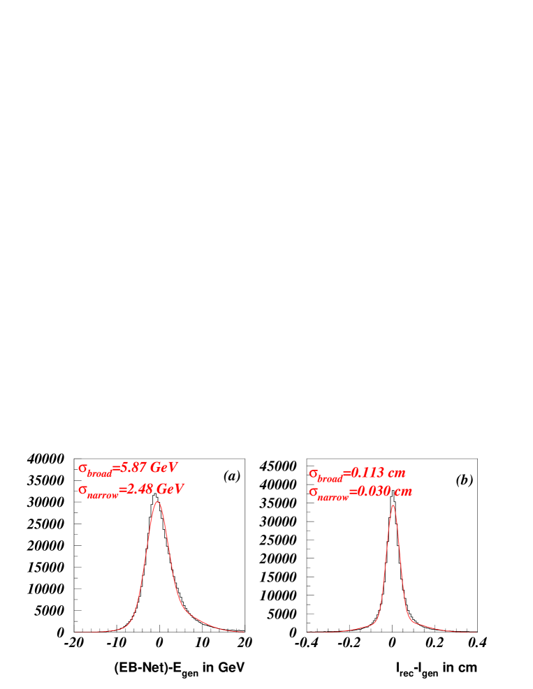
Figure 5: (a) The EB-Net and (b) the reconstructed B-candidate decay length residual i.e. the difference between the reconstructed value and the generated value based on 1994 simulated data.

5.2 Decay Length Reconstruction

Starting from the standard secondary vertex described in Section 4.3, four algorithms were implemented, based on the BD-Net, with the aim of improving the decay length resolution and minimising any bias of the type described in Section 4.5, resulting from the inclusion of tracks from the cascade D-decay vertex in the B-decay vertex reconstruction. In addition to passing the standard quality cuts listed in Section 4.3, tracks were required to have TrackNet values $>0.5$ to be considered for any of the four algorithms.

• In the Strip-Down method candidate tracks were selected if, in addition to the cuts described above, they had BD-Net values $<0.0$. A secondary vertex fit was made if there were two or more tracks selected. If the fit failed to converge (under the same criteria as were applied to the standard fit - see Section 4.3), and more than two tracks were originally selected, the track with the highest $\chi^{2}$ contribution was removed and the fit repeated. This procedure continued iteratively until convergence was reached or less than two tracks were left. Technically, the fit was the same as that used to fit the standard secondary vertex described in Section 4.3 except the starting point was the secondary vertex position estimate of the standard fit.

• In the D-Rejection method, a cascade D-candidate vertex was first built by fitting a common vertex to the two tracks with the largest BD-Net values in the hemisphere. If the invariant mass of the combination was below the D-meson mass, an attempt was made to include also the track with the next largest BD-Net value. This process continued iteratively until either the mass exceeded the D-mass, there were no further tracks, or the fit failed to converge. The B-candidate vertex was then fitted using the Strip-Down algorithm but applied to all tracks except those already selected for the D-vertex.

• In the Build-Up method those two tracks with TrackNet bigger than $0.5$ and smallest BD-Net values were chosen to form a seed vertex. If the invariant mass of all remaining tracks with TrackNet $>0.5$ exceeded the D-mass, that track with the lowest BD-Net output was also fitted to a common vertex with the two seed tracks. This process continued iteratively until either the fit failed to converge or the mass in remaining tracks dropped below the D-meson mass.

• The Semileptonic algorithm was designed to improve the vertex resolution for semileptonic decays of b-hadrons where energy has been carried away by the associated neutrino. When there was a clear lepton candidate in the hemisphere, the algorithm reconstructed a cascade D-candidate vertex in a similar way to the D-rejection method but with the lepton track excluded. The tracks associated with the vertex were then combined to form a ‘D-candidate track’ which was extrapolated back to make the B-candidate vertex with the lepton track if the opening angle between the lepton and D-candidate satisfied $|\cos\Theta_{LD}|<0.99$.

The choice of decay length for the decay time calculation was dictated by optimising the resolution and minimising any bias while still retaining the best possible efficiency. If more than one of the four algorithms was successful in reconstructing a vertex, the choice was made in the following order:

• the Strip-Down method was chosen if the algorithm had a decay length error smaller than 1 mm,

• if the Strip-Down method criteria were not met, the D-rejection method was used if the decay length error was smaller than 1 mm,

• if the criteria for 1) and 2) were not met the Build-Up vertex was chosen if the decay length error was smaller than 200 $\mu{\mathrm{m}}$,

• if the criteria for 1), 2) and 3) were not met the Semileptonic algorithm was used if the decay length error was smaller than 1 mm.

About one third of all hemispheres, passing the event selection cuts, were rejected by the decay length selection procedure in data and in simulation. There were 180010 vertices selected in the 1994 data set and 86796 in 1995. Figure 5(b) plots the residual between the reconstructed decay length and the generated value. A double-Gaussian fit to the distribution gives a central, narrow, Gaussian covering 71% of the total area with a standard deviation of 300 $\mu{\mathrm{m}}$. The lack of a significant positive bias to this distribution, illustrates that the influence of tracks from cascade D-meson decays has been successfully minimised by employing algorithms based on the BD-Net.

6 Selection of ${\mathrm{B}^{+}}$ and ${\mathrm{B}^{0}}$ Enhanced Samples

The enrichment of ${\mathrm{B}^{0}}$ and ${\mathrm{B}^{+}}$ mesons was part of a general attempt to provide a probability for an event hemisphere to contain a b-hadron of a particular type. The result was implemented in a neural network ($NN(B_{x})$) consisting of 16 input variables and a 4-node output layer. Each output node delivered a probability for the hypothesis it was trained on: the first supplied the probability for ${\mathrm{B}}_{{\mathrm{s}}}^{0}$ mesons to be produced in the hemisphere, the second for ${\mathrm{B}^{0}}$ mesons, the third for charged B-mesons and the fourth for all species of b-baryons. The method relied heavily on the reconstruction of the following quantities:

• b-hadron type probabilities $P({\mathrm{B}}_{x})$: supplied by an auxiliary neural network constructed to supply inputs to the more optimal $NN(B_{x})$ network. In common with the $NN(B_{x})$, there were four output nodes trained to return the probability that the decaying b-hadron state was ${\mathrm{B}^{+}}$, ${\mathrm{B}^{0}}$, ${\mathrm{B}}_{{\mathrm{s}}}^{0}$ or b-baryon. There were fifteen input variables in total, the most powerful of which were the hemisphere TrackNet-weighted charge sum, which discriminates charged from neutral states, and variables that exploit the presence of particular particles produced in association with b-hadron states. Examples of this include ${\mathrm{B}}_{{\mathrm{s}}}^{0}$ mesons, which are normally produced with a charged kaon as the leading fragmentation particle with a further kaon emerging from the weak decay, and in ${\mathrm{B}^{+}}$ and ${\mathrm{B}^{0}}$ production where the decay is associated with a larger multiplicity of charged pions than that for ${\mathrm{B}}_{{\mathrm{s}}}^{0}$ and b-baryons (which on average will produce a higher proportion of neutrons, protons and kaons).

• The b-hadron flavour i.e. the charge of the constituent b-quark both at the fragmentation ($F_{frag.}$) and decay time ($F_{dec.}$): knowledge of b-hadron flavour provides the network with valuable information about whether a ${\mathrm{B}^{0}}$ state was present since the fragmentation and decay flavour will, on average, disagree for the case where the ${\mathrm{B}^{0}}$ oscillated. The flavour was determined by first constructing, with neural network techniques, the conditional probability for each charged particle in the hemisphere to have the same charge as the b-quark in the b-hadron. This was repeated separately for each of the four possible b-hadron type scenarios i.e. ${\mathrm{B}^{0}}$,${\mathrm{B}^{+}}$,${\mathrm{B}}_{{\mathrm{s}}}^{0}$ or b-baryon. The flavour network was trained on a target value of $+1(-1)$ if the particle charge was correlated(anti-correlated) to the b-quark charge. The main input variables were those related to the identification of kaons, protons, electrons and muons together with quantities sensitive to the B-D vertex separation in the hemisphere. Tracks originating from the fragmentation (decay) phase were discriminated by checking that the TrackNet value is less (greater) than 0.5. In a final step, these track level probabilities were combined via a likelihood ratio into hemisphere quantities. Providing separate flavour networks for the different b-hadron types not only ensured that the information was optimal for the case of ${\mathrm{B}^{0}}$ but also helped the performance of the enrichment $NN(B_{x})$ network by providing information that was specific to a particular b-hadron type.

The inputs to the $NN(B_{x})$ were constructed to exploit optimally all of the information that the b-hadron production and decay process reveals. The basic construct for input variables was the following combination of the flavour and b-hadron type information described above:

$$F_{dec.}({\mathrm{B}}_{x})\cdot F_{frag.}({\mathrm{B}}_{x})\cdot P({\mathrm{B}}_{x}).$$ (1)

The upper plots of Figure 6 show the output of the ${\mathrm{B}^{+}}$ and ${\mathrm{B}^{0}}$ output nodes of the $NN(B_{x})$ in simulation and data. The simulation is further divided into the different b-hadron types and the lower plots trace the change in purity of the different types in each bin of the network output at the ${\mathrm{B}^{+}}$ and ${\mathrm{B}^{0}}$ output nodes respectively. Note that the background from u,d,s- and c-events is labelled as ‘bg’.

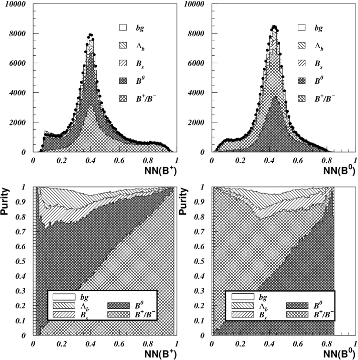
Figure 6: The upper plots show the output of the ${\mathrm{B}^{+}}$ and ${\mathrm{B}^{0}}$ output nodes of the $NN(B_{x})$ in the 1994 data and simulation for the different b-hadron types. The normalisation is to the number of data events and overlaid is the b-hadron composition as seen in the Monte Carlo. The lower plots trace the change in purity of the different b-hadron types, per bin, as a function of cuts on the $NN(B^{+})$ and $NN(B^{0})$ respectively.

7 Extraction of ${\mathrm{B}^{+}}$ and ${\mathrm{B}^{0}}$ Lifetimes

This section describes how the data and simulation samples were prepared, gives details of the fitting procedure itself and summarises the results obtained. Section 7.1 lists corrections made to the default simulation to account for known discrepancies with data and to update b-physics parameters to agree with recent world measurements. In Section 7.2 the final selection and composition of the ${\mathrm{B}^{+}}$, ${\mathrm{B}^{0}}$ and $\tau_{\mathrm{b}}$ samples are described together with an explanation of how the region at low proper times i.e. $<1$ ps was handled in the lifetime fits. Section 7.3 gives technical details of the $\chi^{2}$ fit and presents the results obtained. Lifetimes were measured separately in 1994 and 1995 data and then combined to give the final results which are presented in Section 9.

7.1 Simulation Weighting

Weights were applied to the simulation to correct for the following effects:

• The world average of measurements of ${\mathrm{B}}_{{\mathrm{s}}}^{0}$, ${\mathrm{\Lambda}_{b}}$ lifetimes and b-hadron production fractions, as compiled for the Winter conferences of 2001 [13], listed in Table 1. Note that using more  [13] recent world average values has a negligible effect on the analysis results.

• The Peterson function used in the Monte Carlo ($\langle x\rangle=0.706$) was changed to agree with the functional form unfolded from the 1994 DELPHI data set [12] ($\langle x\rangle=0.7153$).

• A hemisphere ‘quality flag’ which was proportional to the number of tracks in the hemisphere likely to be badly reconstructed e.g. those tracks failing the standard selection criteria of Section 4.3. The weight was constructed to account for data/simulation discrepancies in this variable and was formed in bins of the number of charged particles in the hemisphere, that passed the standard quality cuts of Section 4.3, thus ensuring that, overall, the multiplicity of good charged particles was unchanged after the application of the weight.

b-hadron species	Lifetime	Production fractions $f(b\rightarrow B_{x})$
		Values	$\rho(B_{x},B_{s})$	$\rho(B_{x},baryon)$
${\mathrm{B}}_{{\mathrm{s}}}^{0}$	$1.464\pm 0.057$ps	$f({\mathrm{B}}^{0}_{\mathrm{s}})=0.097\pm 0.011$	-	+0.034
b-baryons	$1.208\pm 0.051$ps	$f({\mathrm{b}aryon})=0.104\pm 0.017$	$+0.034$	-
${\mathrm{B}}_{{\mathrm{d}}}^{0}$ or ${\mathrm{B}^{+}}$	-	$f({\mathrm{B}}^{0}_{\mathrm{d}})=f({\mathrm{B}^{+}})=0.399\pm 0.010$	-0.577	-0.836

Table 1: Values for the b-hadron lifetimes and production fractions (together with correlations) used to re-weight the Monte Carlo.

7.2 Fit working point

The selection conditions imposed on the data samples used for the lifetime fits were motivated by the wish to minimise the total error on the final results. Systematic error contributions due to inexact detector resolution simulation and the physics modelling of u,d,s and charm production, imply that relatively high b-hadron purities were required while still keeping the selection efficiency above a level where the statistical error would begin to degrade significantly.

With these considerations in mind, the final data samples to be used in the fitting procedure were selected by cutting on the $NN(B_{x})$ neural network outputs, described in Section 6, at $>0.52$ and $>0.6$ respectively to obtain enhanced samples in ${\mathrm{B}^{+}}$ and ${\mathrm{B}^{0}}$. These cut values corresponded to a purity in both ${\mathrm{B}^{+}}$ and ${\mathrm{B}^{0}}$ of approximately $70\%$ according to the simulation. No reconstructed hemisphere passed both the ${\mathrm{B}^{+}}$ and ${\mathrm{B}^{0}}$ enhancement cuts simultaneously and hence the two samples were statistically independent.

The region below about $1.0$ ps in proper lifetime is particularly challenging to simulate. The modelling of very small lifetimes is rather sensitive to details of reconstruction resolution and the modelling of events which contain no intrinsic lifetime information such as u,d,s events and the reconstruction or spurious vertices. In addition, the lower plots of Figures 7 and 8 show that the purities of the different b-hadron types is rapidly changing in this region, making them particularly difficult to model. These issues meant that the low lifetime region was not well enough under control systematically for precision lifetime information to be extracted and the region below $1.0$ ps was therefore excluded from the analysis. This point is illustrated in Figure 10 which shows that the fit results only become stable in all samples for a fit starting point larger than $1.0$ ps.

After all selection cuts already described, the size and composition of the ${\mathrm{B}^{+}}$and ${\mathrm{B}^{0}}$ enhanced samples are summarised in Table 2. The ${\mathrm{B}^{+}}$(${\mathrm{B}^{0}}$) sample sizes correspond to a selection efficiency, with respect to the starting number of ${\mathrm{B}^{+}}$ and ${\mathrm{B}^{0}}$ states in the hadronic sample, of 10.1%(3.8%) for both 1994 and 1995 data.

	${\mathrm{B}^{+}}$ Sample	${\mathrm{B}^{0}}$ Sample
Real data sample size 1994(1995)	27356(13150)	9293(4335)
Simulation sample size 1994(1995) $q\bar{q}$	61821(23415)	22667(8533)
Simulation sample size 1994(1995) $b\bar{b}$	161198(42951)	59015(15863)
${\mathrm{B}^{+}}$ fraction	$71.7\%$	$15.8\%$
${\mathrm{B}^{0}}$ fraction	$20.7\%$	$68.5\%$
${\mathrm{B}}_{{\mathrm{s}}}^{0}$ fraction	$3.7\%$	$10.1\%$
b-baryon fraction	$2.4\%$	$4.4\%$
u,d,s fraction	$0.2\%$	$0.1\%$
c fraction	$1.2\%$	$1.0\%$

Table 2: The ${\mathrm{B}^{+}}$ and ${\mathrm{B}^{0}}$ sample size in data and simulation and the composition of the simulation. The simulation has been weighted for the quantities listed in Section 7.1.

The data sample used to fit for the mean b-hadron lifetime passed through the same event selection and proper time cuts as for the ${\mathrm{B}^{+}}$ and ${\mathrm{B}^{0}}$ samples but without any requirement on the $NN(B_{x})$ neural network outputs. The size and composition of the mean b-hadron sample is summarised in Table 3. These numbers imply that the mean lifetime measurement is valid for a b-hadron mixture, as given by the simulation, of ${\mathrm{B}^{+}}$$=41.9\%$, ${\mathrm{B}^{0}}$$=41.2\%$, ${\mathrm{B}}_{{\mathrm{s}}}^{0}$$=8.9\%$ and b-baryon$=8.0\%$.

	b-hadron
Sample size 1994(1995)	114317(54958)
Simulation sample size 1994(1995) $q\bar{q}$	262697(98230)
Simulation sample size 1994(1995) $b\bar{b}$	677998(180634)
${\mathrm{B}^{+}}$ fraction	$41.2\%$
${\mathrm{B}^{0}}$ fraction	$40.5\%$
${\mathrm{B}}_{{\mathrm{s}}}^{0}$ fraction	$8.7\%$
b-baryon fraction	$7.7\%$
u,d,s fraction	$0.3\%$
c fraction	$1.7\%$

Table 3: The mean b-hadron sample size in data and simulation and the composition of the simulation. The simulation has been weighted for the quantities listed in Section 7.1.

7.3 Lifetime Results

The ${\mathrm{B}^{+}}$, ${\mathrm{B}^{0}}$ and $\tau_{\mathrm{b}}$ lifetimes were extracted by fitting the simulated proper time distribution to the same distribution formed in the data using a binned $\chi^{2}$ method. As discussed in Section 7.2 the start point of the fit range was chosen to be $1$ ps. The upper limit was positioned to avoid the worst effects of spurious, mainly two-track vertices, with very long reconstructed lifetimes while still accepting the vast majority of the data available. Nominally 100 bins were chosen but the exact binning was determined by the requirement that at least 10 entries be present in all bins of the data distribution.

To avoid the need to generate many separate Monte Carlo samples with different B-lifetimes, weighting factors were formed for each lifetime measurement from the ratio of exponential decay probability functions. Specifically, the weight,

$$w_{i}=\frac{\tau_{old}}{\tau_{new}}exp\left(\frac{t_{i}(\tau_{new}-\tau_{old})}{\tau_{old}\tau_{new}}\right),$$

for measurement $i$ and true B-lifetime $t_{i}$, effectively transforms the Monte Carlo lifetimes generated with a mean lifetime $\tau_{old}$ to be distributed with a new mean value of $\tau_{new}$. Throughout the fit for the ${\mathrm{B}^{+}}$ and ${\mathrm{B}^{0}}$ lifetimes, the ${\mathrm{B}_{s}}$ and ${\mathrm{\Lambda}_{b}}$ lifetime components were weighted to the current world average numbers listed in Table 1 and for the $\tau_{\mathrm{b}}$ fit, the starting value in the simulation was $1.6\,$ps. The $\chi^{2}$ function given below was then minimised with respect to the ${\mathrm{B}^{+}}$ and ${\mathrm{B}^{0}}$ lifetimes in a simultaneous two parameter fit or to the mean b-hadron lifetime $\tau_{\mathrm{b}}$ in a one parameter fit,

$$\chi^{2}=\sum_{{\mathrm{B}}^{0},{\mathrm{B}}^{+}}\left[\sum_{i=1}^{n_{bins}}\frac{(W^{sim}_{i}-N^{data}_{i})^{2}}{(\sigma^{sim}_{i})^{2}+(\sigma^{data}_{i})^{2}}\right].$$

Here, $N^{data}_{i}$ is the number of data entries in bin $i$ and $W^{sim}_{i}$ is the corresponding sum of weights in bin $i$ of the simulation.

The results from all lifetime fits, after imposing the working point conditions and following the above procedure, are listed in Table 4. In the table, the first error quoted is statistical and the second systematic. The various sources of systematic error are described in Section 8. Results are given for 1994 and 1995 data separately and combined taking into account correlated systematic errors as described in Section 9.

b-State	Fitted Lifetime
	’94	’95	Combined
${\mathrm{B}^{+}}$	$1.624\pm 0.017\pm 0.023$ ps	$1.623\pm 0.025\pm 0.019$ ps	$1.624\pm 0.014\pm 0.018$ ps
${\mathrm{B}^{0}}$	$1.548\pm 0.026\pm 0.035$ ps	$1.497\pm 0.039\pm 0.041$ ps	$1.531\pm 0.021\pm 0.031$ ps
$\frac{\tau_{{\mathrm{B}}^{+}}}{\tau_{{\mathrm{B}}^{0}}}$	$1.049\pm 0.025\pm 0.027$	$1.085\pm 0.040\pm 0.036$	$1.060\pm 0.021\pm 0.024$
$\tau_{\mathrm{b}}$	$1.577\pm 0.006\pm 0.008$ ps	$1.555\pm 0.009\pm 0.011$ ps	$1.570\pm 0.005\pm 0.008$ ps

Table 4: The results of the lifetime fits in the 1994 and 1995 data samples where the first error quoted is statistical and the second systematic.

The ${\mathrm{B}^{+}}$ and ${\mathrm{B}^{0}}$ fits (to the 1994 data) are shown in Figure 7. The correlation coefficient between ${\mathrm{B}^{+}}$ and ${\mathrm{B}^{0}}$ lifetimes was found to be $-0.51$ for both the 1994 and 1995 fits. The fit $\chi^{2}$ at the minimum point was $178$ for $160$ degrees of freedom for 1994 data and $142$ for $143$ degrees of freedom for 1995 data.

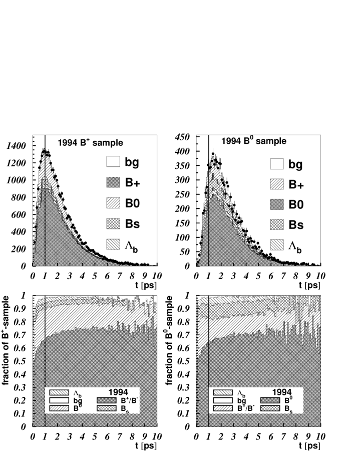
Figure 7: The upper two plots show the result of the fit in the ${\mathrm{B}^{+}}$(left) and ${\mathrm{B}^{0}}$(right) samples in 1994(histogram) compared to data(points). The b-hadron composition of the ${\mathrm{B}^{+}}$ and ${\mathrm{B}^{0}}$ sample is also indicated where ‘bg’ refers to the background from non-${\mathrm{b}}\bar{{\mathrm{b}}}$ ${\mathrm{Z}}^{0}$ decays. The lower two plots trace how the fractional composition of the sample changes in bins of the reconstructed lifetime. The vertical line at $t=1\,\mathrm{ps}$ indicates that data below this point are removed from the analysis.

The mean b-hadron lifetime fit is shown in Figure 8. The $\chi^{2}$ at the minimum point was $76$ for $88$ degrees of freedom in 1994 data and $70$ for $88$ degrees of freedom for 1995 data.

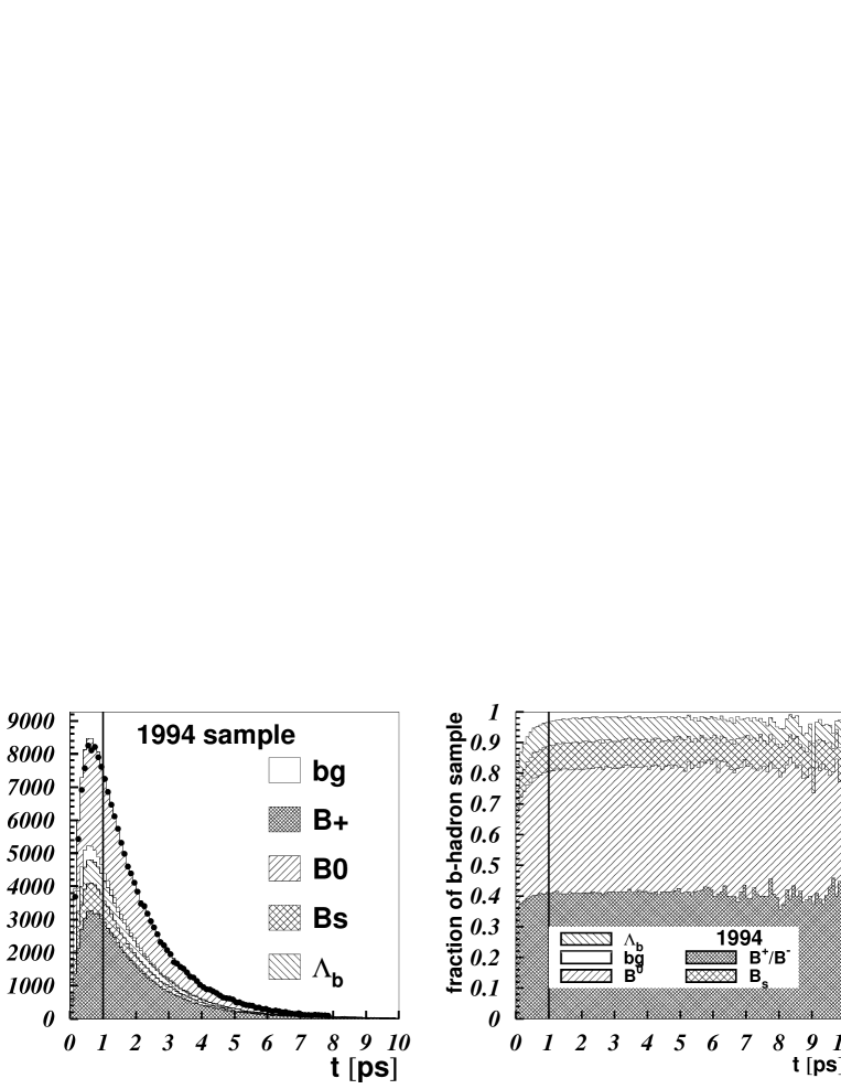
Figure 8: The left plot shows the result of the mean $b$-hadron lifetime fit in 1994 (histogram) compared to the data(points) at the working point. The right plot traces how the fractional composition varies in bins of the reconstructed lifetime. The vertical line at $t=1\,\mathrm{ps}$ indicates that data below this point are removed from the analysis.

Figure 9 illustrates the effect of cut scans in the ${\mathrm{Z}}^{0}\rightarrow{\mathrm{b}}\bar{{\mathrm{b}}}$ event purity (i.e. the estimated fraction of the data sample fitted coming from ${\mathrm{Z}}^{0}\rightarrow{\mathrm{b}}\bar{{\mathrm{b}}}$ events) showing a good stability over a wide range of the cut values for the lifetime ratio $\tau(B^{+})/\tau(B^{0})$ and the mean b-hadron lifetime. Similarly Figure 10 illustrates that the results are very stable over a wide range of different start points for the fits above the default cut point of $t=1\,$ps.

A further crosscheck on the results was made by repeating the fits for one data set using the simulation sample compatible with another data set e.g. fitting 1994 data using 1995 simulation. It was found that all fit results (for ${\mathrm{B}^{+}}$, ${\mathrm{B}^{0}}$ and $\tau_{\mathrm{b}}$) for both cases (1994 data using 1995 simulation and 1995 data using 1994 simulation) changed by amounts that were within the systematic error for detector effects quoted in Table 5 which provides a rough check that aspects of detector and physics modelling are well under control.

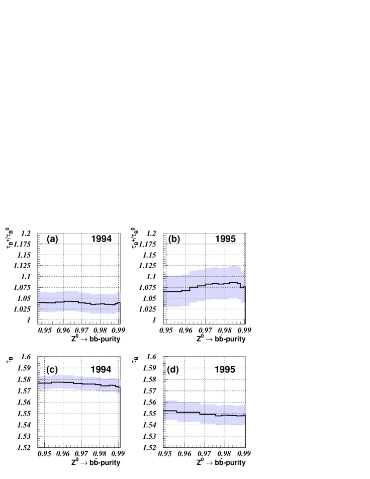
Figure 9: The variation in the fitted lifetimes as a function of the ${\mathrm{Z}}^{0}\rightarrow{\mathrm{b}}\bar{{\mathrm{b}}}$ purity for the ratio $\tau(B^{+})/\tau(B^{0})$ in (a) 1994 and (b) 1995 data and for the mean b-hadron lifetime in (c) 1994 and (d) 1995 data. The upper and lower shaded bands represent the statistical one standard deviation errors which are correlated bin-to-bin.

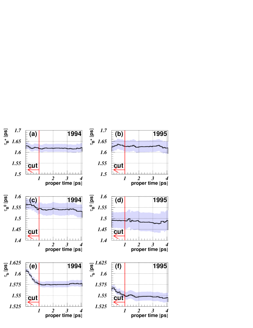
Figure 10: Lifetime fit results as a function of varying the start point of the fit for ${\mathrm{B}^{+}}$ in (a) 1994 and (b) 1995, ${\mathrm{B}^{0}}$ in (c) 1994 and (d) 1995 and for the mean b-hadron fit in (e) 1994 and (f) 1995.

8 Systematic Uncertainties

Systematic uncertainties on the lifetime measurements come from three main sources. The first source is from the modelling of heavy flavour physics parameters in our Monte Carlo generator. Since attempts were made to model these effects using current world averages, these errors are largely irreducible. The second source comes from the analysis method itself and the choices made in determining the measurement working point. The good level of agreement between simulation and data and the fact that the result is stable within a wide range of the working point (e.g. as shown in Figure 9) mean that these errors are kept to a minimum. The third source of systematic uncertainty can be generically termed ‘detector effects’ and results from a less-than-perfect modelling in simulation of the response of the detector.

Tables 5 and 6 present the full systematic error breakdown for the measurements of $\tau({\mathrm{B}}^{+})$, $\tau({\mathrm{B}}^{0})$ and $\tau_{\mathrm{b}}$ in 1994 and 1995 data.

8.1 Heavy Flavour Physics Modelling

Where possible, B-physics modelling uncertainties were estimated by varying central values by plus and minus one standard deviation and taking half of the observed change in the fitted lifetime value as the resulting systematic uncertainty from that source.

The ${\mathrm{B}}_{{\mathrm{s}}}^{0}$, b-baryon lifetimes, b-hadron production fractions and fragmentation $\left<x\right>$ value have been varied within their errors as listed in Section 7.1 and half of the full variation in the results has been assigned as an error. In the case of the b-hadron production fractions, the variation was made taking into account correlations from the covariance matrix listed in Table 1.

   $\tau_{{\mathrm{B}}^{+}}\,(1994|1995)$    $\tau_{{\mathrm{B}}^{0}}\,(1994|1995)$    $\frac{\tau_{{\mathrm{B}}^{+}}}{\tau_{{\mathrm{B}}^{0}}}\,(1994|1995)$ Result [ps] 1.6241 1.6233 1.5483 1.4971 1.0492 1.0848 Statistical Error [ps] 0.0168 0.0251 0.0255 0.0388 0.0247 0.0398 Source of Systematic Error       Range    $\Delta\tau_{{\mathrm{B}}^{+}}$ [ps]    $\Delta\tau_{{\mathrm{B}}^{0}}$ [ps]    $\Delta\frac{\tau_{{\mathrm{B}}^{+}}}{\tau_{{\mathrm{B}}^{0}}}$ Physics Modelling ${\mathrm{B}}_{s}$ lifetime $1.464\pm 0.057$ ps 0.0007 0.0080 0.0050 ${\mathrm{b}}$-baryon lifetime $1.208\pm 0.051$ ps 0.0007 0.0030 0.0028 ${\mathrm{b}}$-hadron prod. fractions See text 0.0035 0.0035 0.0004 Fragmentation function $\left<x\right>=0.7153\pm 0.0052$ [12] 0.0037 0.0026 0.0040 ${\mathrm{B}}\rightarrow{\mathrm{D}X}$ branching fractions See text 0.0081 0.0086 0.0017 BR(${\mathrm{B}}\rightarrow$ wrong-sign charm) $20.0\%\pm 3.3\%$ 0.0030 0.0047 0.0014 BR(${\mathrm{B}_{s}}\rightarrow{\mathrm{D}_{s}}$) $35\%\rightarrow 70\%$ 0.0017 0.0076 0.0062 BR$({\mathrm{b}}\rightarrow$c-baryon X) $9.6\%\pm 3.0\%$ 0.0009 0.0032 0.0016 ${\mathrm{D}^{+}},{\mathrm{D}^{0}}$ topo. branching ratios [14] 0.0016 0.0113 0.0084 B meson mass $m_{B}=5.2789\pm 0.0018~{}\mathrm{Gev/c^{2}}$ 0.0004 0.0015 0.0011 b-hadron Reconstruction b and c efficiency correction On/off 0.0076 0.0048 0.0050 0.0066 0.0015 0.0017 $NN(B_{x})$ cuts 65%-75% purity 0.0093 0.0133 0.0216 0.0255 0.0196 0.0269 $NN(B_{x})$ shape See text 0.0008 0.0006 0.0099 0.0126 0.0059 0.0097 Sec. vertex multiplicity See text 0.0022 0.0019 0.0042 0.0040 0.0040 0.0042 Detector Effects Resolution and On/off 0.0171 0.0075 0.0144 0.0200 0.0110 0.0159 hemisphere quality Total Systematic Error 0.0234 0.0192 0.0345 0.0406 0.0269 0.0355

Table 5: Summary of systematic uncertainties in the ${\mathrm{B}^{+}}$and ${\mathrm{B}^{0}}$ lifetime results and their ratio for 1994 and 1995 data. Systematic errors are assumed independent and added in quadrature to give the total systematic error quoted.

		$\tau_{{\mathrm{B}}}$ for 1994	$\tau_{{\mathrm{B}}}$ for 1995
Result [ps]		1.5773	1.5546
Statistical Error [ps]		0.0059	0.0085
Source of Systematic Error	Range	$\Delta\tau_{{\mathrm{B}}}$ [ps]	$\Delta\tau_{{\mathrm{B}}}$ [ps]
Physics Modelling
${\mathrm{b}}$-hadron prod. fractions	See text	0.0011
Fragmentation function	$\left<x\right>=0.7153\pm 0.0052$ [12]	0.0038
BR(${\mathrm{B}}\rightarrow$ wrong-sign charm)	$20\%\pm 3.3\%$	0.0010
BR(${\mathrm{B}_{s}}\rightarrow{\mathrm{D}_{s}}$)	$35\%\rightarrow 70\%$	0.0012
BR$({\mathrm{b}}\rightarrow$c-baryon X)	$9.6\%\pm 3.0\%$	0.0017
${\mathrm{B}}\rightarrow{\mathrm{D}X}$ branching fractions	See text	0.0008
${\mathrm{D}^{+}},{\mathrm{D}^{0}}$ topo. branching ratios	See text	0.0008
B-meson mass	$m_{B}=5.2789\pm 0.0018~{}\mathrm{Gev/c^{2}}$	0.0004
b-hadron Reconstruction
b and c efficiency correction	On/off	0.0057	0.0048
Sec. vertex multiplicity	See text	0.0019	0.0023
Detector Effects
Resolution and	See text	0.0035	0.0083
hemisphere quality
Total Systematic Error		0.0084	0.0109

Table 6: Summary of systematic uncertainties in the mean b-hadron lifetime for 1994 and 1995 data. Systematic errors are assumed independent and added in quadrature to give the total systematic error.

Close attention was paid to possible systematic effects on the analysis due to the modelling of ${\mathrm{b}}\rightarrow$ charm branching ratios, where current experimental knowledge is scarce. The charm content impacts on the performance of the ${\mathrm{B}}^{+}$ and ${\mathrm{B}^{0}}$ enhancement networks and can pull the reconstructed B-vertex position to longer decay lengths. The size of this pull in turn depends on whether a ${\mathrm{D}}^{0}$ or ${\mathrm{D}}^{+}$ was produced since $\tau({\mathrm{D}}^{+})\sim 2.5$ times larger than $\tau({\mathrm{D}}^{0})$. Specific aspects of the Monte Carlo that were found to warrant systematic error contributions were:
(a) Inclusive, ${\mathrm{B}}\rightarrow{\mathrm{D}}$ branching ratios were adjusted in the Monte Carlo according to a fit using all currently available measurements from [2] as constraints. The values taken were: $BR\left(\bar{{\mathrm{B}}}^{0}\rightarrow{\mathrm{D}}^{+}X\right)=15.6\%$, $BR\left(\bar{\mathrm{B}}^{0}\rightarrow{\mathrm{D}}^{0}X\right)=65.8\%$, $BR\left({\mathrm{B}}^{-}\rightarrow{\mathrm{D}}^{+}X\right)=29.3\%$, $BR\left({\mathrm{B}}^{-}\rightarrow{\mathrm{D}}^{0}X\right)=52.1\%$. The full difference seen in the results due to this change was assigned as a systematic error.
(b) The standard Monte Carlo data set used contained a wrong-sign charm production rate into ${\mathrm{D}_{s}}$ of $11\%$. This rate is now known to be too low due to the production of ${\mathrm{D}}^{0}/{\mathrm{D}}^{+}$ mesons at the $W$ vertex (in addition to ${\mathrm{D}_{s}}$), and an estimate of the overall rate based on [15] is BR(wrong-sign)$=20.0\%\pm 3.3\%$. To account for this discrepancy with current measurements, the wrong-sign rate in the simulation was weighted up to $20.0\%$ and all quoted lifetime results were shifted to be valid for this higher wrong-sign rate. An error was then assigned based on the change in the lifetime results observed when the wrong-sign rate was further changed by $\pm 3.3\%$. The impact of the simulation containing only wrong-sign ${\mathrm{D}_{s}}$ mesons instead of a mixture of ${\mathrm{D}_{s}},{\mathrm{D}}^{0}$ and ${\mathrm{D}}^{+}$ was tested with specially generated Monte Carlo data sets, and the effect found to be small compared to the overall effect of having almost double the rate of events containing two D-mesons per hemisphere.
(c) BR$({\mathrm{B}_{s}}\rightarrow{\mathrm{D}_{s}}$X) is currently known to, at best, $\pm 30$% [2] and was varied in the Monte Carlo by a factor two from the default value of $35\%$. The full change in the fitted lifetime was then assigned as a systematic error.
(d) BR$({\mathrm{b}}\rightarrow$c-baryon X), where b represents the natural mixture of b-mesons and baryons at LEP, was varied from the default value in the simulation of $9.6\%$ by $\pm 3.0\%$. This range covers the uncertainty on this quantity from experiment which currently stands at BR$({\mathrm{b}}\rightarrow$c-baryon X)$=9.7\pm 2.9\%$ [2]. Half of the full change in the fitted lifetime was then assigned as a systematic error.

The uncertainty from D-topological branching fractions was estimated from the difference in the fit result obtained when weighting according to the results from [14]. The masses of B-mesons were varied within plus and minus one standard deviation of the value assumed in the BSAURUS package and half of the change seen taken as a systematic error.

Since many of the physics modelling systematics investigated are significantly smaller than the statistical precision, the approach was taken to average the errors, evaluated in 1994 and 1995 data, weighted by the statistical error for each year. This ensures that the effects of statistical fluctuations in the determination of these errors are minimised and explains why the physics modelling errors appearing in Table 5 are the same for 1994 and 1995.

8.2 b-hadron Reconstruction

The efficiency for reconstructing ${\mathrm{b}}\bar{{\mathrm{b}}}$ and ${\mathrm{c}}\bar{{\mathrm{c}}}$ events (as a function of the event b-tag) has been extracted from the real data by a double-hemisphere tagging technique. At the b-tag value of the working point, the results of this study suggest that while the reconstruction efficiency for ${\mathrm{b}}\bar{{\mathrm{b}}}$ events might be underestimated in the simulation by about $\sim 2\%$ (relative), the efficiency for ${\mathrm{c}}\bar{{\mathrm{c}}}$ events in simulation is $\sim 8\%$ (relative) lower than in data. To account for this possible source of error the difference seen in the fit results, when these efficiencies were changed in the simulation to agree with the numbers above, was assigned as a systematic error. Since a large part of the discrepancy between simulation and data in the ${\mathrm{c}}\bar{{\mathrm{c}}}$ event reconstruction efficiency is due to a less-than-perfect modelling of charm physics, this error contribution has already been partially accounted for by the explicit charm physics systematics detailed above. Given the current level of uncertainty in this sector, the conservative approach of quoting both error contributions is preferred.

As was remarked in Section 7.3, uncertainties resulting from the method itself have been checked by scanning regions around critical cut values to check for stability as illustrated in Figure 9. In addition, the binning used for the $\chi^{2}$ formulation was varied over a wide range as was the minimum number of entries per bin (set by default to 10) and were both found to give no significant change in the results.

The impact on the analysis of any residual discrepancy between data and simulation in the BD-Net variable was checked by studying the effect of removing the Strip-Down vertex algorithm (see Section 5.2) from the analysis. Of the four vertex algorithms used, the Strip-Down method is the most sensitive to details of the BD-Net variable since it imposes a direct cut in the BD-Net as part of the track selection. Removing the Strip-Down algorithm and replacing it with one of the other three methods, selected by the same criteria as described in Section 5.2, resulted in lifetime results for 1994 data that changed by $\Delta\tau(B^{+})=-0.0017$ ps and $\Delta\tau(B^{0})=-0.0063$ ps i.e. well within the total systematic error quoted. In addition it was confirmed that the proper time distributions were well compatible when the cut imposed on the BD-Net distribution was changed from the default value of zero to $\pm 0.2$.

The analysis assumes that the ${\mathrm{B}^{+}}$ and ${\mathrm{B}^{0}}$ purities are well modelled by the simulation. A systematic error will arise if the shape of the $NN(B^{+})$ and $NN(B^{0})$ network outputs differ from the data and/or the composition of the ${\mathrm{B}^{+}}$ and ${\mathrm{B}^{0}}$ simulated samples differ. Any difference in shape between data and simulation was accounted for in the following way. It was assumed that the difference could be wholly accounted for by a change in just the ${\mathrm{B}^{+}}$ composition for the case of the $NN(B^{+})$ network and by just the ${\mathrm{B}^{0}}$ composition for the case of the $NN(B^{0})$ network. In this way it was found that the maximum error made by assuming that the ${\mathrm{B}^{+}}$ and ${\mathrm{B}^{0}}$ purities in the simulation were correct, was of order 2% and 4%, respectively. The effect of these changes were then propagated into errors on the extracted lifetimes. To account for any composition differences, half of the maximum variation in the fitted lifetime while scanning the purity range $\left[65\%,75\%\right]$ was assigned as an error. The scan range was chosen to enclose the largest uncertainty on the purity found from analysing the shapes of the network outputs described above.

The multiplicity of tracks in the reconstructed b-hadron vertex was found to be in overall good agreement between the data and simulation. To account for any residual differences a weight was formed from the ratio of the data and simulation distributions and the change seen as a result of applying this weight was assigned as a systematic error.

8.3 Detector Modelling

In order to account for uncertainties in the simulation originating from detector response modelling, the effect of switching on and off the following corrections was studied:

• the hemisphere quality weight, described in Section 7.1,

• an attempt to obtain a better match of the track impact parameter and error (with respect to the primary vertex) between simulation and data according to the prescription detailed in [7].

Since in general, knowledge of detector modelling uncertainties are not at the same level of understanding as e.g. our knowledge of the difference between the B-production fractions in our Monte Carlo and the world averages, the following approach was taken to assigning systematic values for these effects: all four combinations of switching these corrections on/off for the ${\mathrm{B}^{+}}$/${\mathrm{B}^{0}}$ fit and the $\tau_{\mathrm{b}}$ analysis were made and the fitted lifetimes of the four possibilities recorded. The central results for ${\mathrm{B}^{+}}$,${\mathrm{B}^{0}}$ and $\tau_{\mathrm{b}}$ were then chosen to be the mean values of these four combinations, and the resulting systematic error from detector response modelling was assigned to be half of the maximum spread of the values recorded from the four combinations. This error is listed in tables 5 and 6 as ‘Resolution and hemisphere quality’.

8.4 Closing Remarks on Systematic Errors

In general it can be concluded from Tables 5 and 6 that detector effects dominate. Physics modelling errors come essentially only from b-physics sources, since the contamination from light-quark and charm events is so small, and are generally well under control. For the case of the ${\mathrm{B}^{+}}$ and ${\mathrm{B}^{0}}$, additional systematic error contributions arising from the enhancement neural networks ( $NN(B_{x})$) reflect the difficult task of modelling accurately such complex variables.

9 Summary and Conclusion

The lifetimes of ${\mathrm{B}^{+}}$, ${\mathrm{B}^{0}}$, their ratio and the mean b-hadron lifetime have been measured. The analysis isolated b-hadron candidates with neural network techniques trained to exploit the physical properties of inclusive b-hadron decays. Binned $\chi^{2}$ fits to the resulting DELPHI data samples collected in 1994 and 1995 yielded the results presented in Table 5 for ${\mathrm{B}^{+}}$ and ${\mathrm{B}^{0}}$ and the result for the mean b-hadron lifetime is presented in Table 6. The results for 1994 and 1995 were combined, treating all systematic contributions as independent apart from the following (which were assumed to be $100\%$ correlated):

• all physics modelling errors,

• the $NN(B_{x})$ shape error,

• the secondary vertex multiplicity error.

The combined results for the ${\mathrm{B}^{+}}$ and ${\mathrm{B}^{0}}$ were,

$\tau_{{\mathrm{B}}^{+}}$	=	1.624	$\pm 0.014$ (stat)	$\pm 0.018$ (syst) ps
$\tau_{{\mathrm{B}}^{0}}$	=	1.531	$\pm 0.021$ (stat)	$\pm 0.031$ (syst) ps
$\frac{\tau_{{\mathrm{B}}^{+}}}{\tau_{{\mathrm{B}}^{0}}}$	=	1.060	$\pm 0.021$ (stat)	$\pm 0.024$ (syst)

and for the average b-hadron lifetime:

$\tau_{{\mathrm{b}}}$

=

1.570

$\pm 0.005$ (stat)

$\pm 0.008$ (syst) ps.

(Note that the average b-hadron lifetime result is valid for a b-hadron mixture, as given by the simulation, of ${\mathrm{B}^{+}}$$=41.9\%$, ${\mathrm{B}^{0}}$$=41.2\%$, ${\mathrm{B}}_{{\mathrm{s}}}^{0}$$=8.9\%$ and b-baryon$=8.0\%$).

These results are well compatible with previous DELPHI results in this area using the 1991-1993 data sets: based on ${\rm D}^{(*)}\ell$ reconstruction [16] and [17] and from an inclusive secondary vertex approach [18]. No attempt has been made to combine these older results with the current analysis because of the vast difference in precision e.g. the error on the lifetime ratio $\frac{\tau_{{\mathrm{B}}^{+}}}{\tau_{{\mathrm{B}}^{0}}}$ is now a factor five better than was achieved in [18].

Compared to existing measurements, the ${\mathrm{B}^{+}}$ lifetime result is currently the most accurate and is well compatible with all other measurements and with the world average value of $1.671\pm 0.018$ ps [2]. The precision of the ${\mathrm{B}^{0}}$ lifetime result is similar to the best so far achieved from ${\mathrm{Z}}^{0}$ data i.e. from an OPAL analysis based on inclusive ${\rm D}^{(*)}\ell$ reconstruction ($1.541\pm 0.028\pm 0.023$ ps [19]) and to recent results from the B-factory experiments, BABAR [20] and BELLE [21]. In addition, the ${\mathrm{B}^{0}}$ lifetime result is well compatible with all other measurements and with the current world average value of $1.537\pm 0.015$ ps [2]. All published measurements of the lifetime ratio $\frac{\tau_{{\mathrm{B}}^{+}}}{\tau_{{\mathrm{B}}^{0}}}$ are presented in Table 7 together with their average [2].

Experiment	Method	Data set	Ratio $\tau_{{\rm B}^{+}}/\tau_{{\rm B}^{0}}$	Reference
ALEPH	D${}^{(*)}\ell$	91-95	1.085$\pm 0.059\pm 0.018$	[22]
ALEPH	Exclusive rec.	91-94	1.27${}^{+0.23+0.03}_{-0.19-0.02}$	[23]
CDF	D${}^{(*)}\ell$	92-95	1.110$\pm 0.056^{+0.033}_{-0.030}$	[24]
CDF	Excl. ($J/\psi K$)	92-95	1.093 $\pm$ 0.066 $\pm$ 0.028	[25]
DELPHI	D${}^{(*)}\ell$	91-93	1.00${}^{+0.17}_{-0.15}\pm$ 0.10	[16]
DELPHI	Charge sec. vtx.	91-93	1.06${}^{+0.13}_{-0.11}\pm 0.10$	[18]
L3	Charge sec. vtx.	94-95	1.09$\pm$ 0.07 $\pm$ 0.03	[26]
OPAL	D${}^{(*)}\ell$	91-93	0.99$\pm 0.14^{+0.05}_{-0.04}$	[27]
OPAL	Charge sec. vtx.	93-95	1.079$\pm$ 0.064 $\pm$ 0.041	[28]
SLD	Charge sec. vtx. $\ell$	93-95	1.03${}^{+0.16}_{-0.14}\pm$ 0.09	[29]
SLD	Charge sec. vtx.	93-95	1.01${}^{+0.09}_{-0.08}\pm$ 0.05	[29]
BABAR	Exclusive rec.	99-00	1.082 $\pm$ 0.026$\pm$ 0.012	[30]
BELLE	Exclusive rec.	99-01	1.091 $\pm$ 0.023$\pm$ 0.014	[21]
Average			1.085 $\pm$ 0.017

Table 7: Measurements of the ratio $\tau_{{\rm B}^{+}}/\tau_{{\rm B}^{0}}$.

It can be seen that the result from this analysis is currently the most precise of the measurements from ${\mathrm{Z}}^{0}$ decay data and the CDF experiment at the Tevatron and also has a precision comparable to the B-factory experiments BABAR and BELLE. Within the quoted errors the result is also compatible with all measurements and with the world average value.

The result for the mean b-hadron lifetime significantly improves on the most precise existing measurement from L3, $\tau_{{\mathrm{b}}}=1.556\pm 0.010\pm 0.017$ ps [32] and is in good agreement with the most precise previous DELPHI publication on this subject [33]. In addition it is compatible with the current world average, $1.564\pm 0.014$ ps [2], which has been compiled assuming that all measurements are based on b-hadron samples with the same mixture of b-hadron species i.e. the b-hadron production fractions from $\rm{Z^{0}}$ decay. It is also informative to compare these values with the inclusive lifetime defined as,
$\tau_{\rm b}=\sum_{i}f({\rm B}_{i})\tau({\rm B}_{i})$, calculated using the current world average values for b-hadron production fractions $f({\rm B}_{i})$ and lifetimes $\tau({\rm B}_{i})$ from [2]: $\tau_{\rm b}=1.543$ ps.

Acknowledgements

We are greatly indebted to our technical collaborators, to the members of the CERN-SL Division for the excellent performance of the LEP collider, and to the funding agencies for their support in building and operating the DELPHI detector.
We acknowledge in particular the support of
Austrian Federal Ministry of Education, Science and Culture, GZ 616.364/2-III/2a/98,
FNRS–FWO, Flanders Institute to encourage scientific and technological research in the industry (IWT), Belgium,
FINEP, CNPq, CAPES, FUJB and FAPERJ, Brazil,
Czech Ministry of Industry and Trade, GA CR 202/99/1362,
Commission of the European Communities (DG XII),
Direction des Sciences de la Mati$\grave{\mbox{\rm e}}$re, CEA, France,
Bundesministerium f$\ddot{\mbox{\rm u}}$r Bildung, Wissenschaft, Forschung und Technologie, Germany,
General Secretariat for Research and Technology, Greece,
National Science Foundation (NWO) and Foundation for Research on Matter (FOM), The Netherlands,
Norwegian Research Council,
State Committee for Scientific Research, Poland, SPUB-M/CERN/PO3/DZ296/2000, SPUB-M/CERN/PO3/DZ297/2000, 2P03B 104 19 and 2P03B 69 23(2002-2004)
JNICT–Junta Nacional de Investigação Científica e Tecnol$\acute{\mbox{\rm o}}$gica, Portugal,
Vedecka grantova agentura MS SR, Slovakia, Nr. 95/5195/134,
Ministry of Science and Technology of the Republic of Slovenia,
CICYT, Spain, AEN99-0950 and AEN99-0761,
The Swedish Natural Science Research Council,
Particle Physics and Astronomy Research Council, UK,
Department of Energy, USA, DE-FG02-01ER41155.

References

[1]
I.I. Bigi et al. in B Decays 2nd edition, ed. S. Stone, World
Scientific (1994); A. Lenz, talk given at the Workshop on the CKM Unitarity Triangle,
CERN, Feb. 13th-16th 2002,
http://ckm-workshop.web.cern.ch/ckm-workshop and hep-ph/0304132/.
[2] K. Hagiwara et al: Phys. Rev. D 66, 010001 (2002)
and 2003 off-year partial update for the 2004 edition available on the PDG WWW pages (URL: http://pdg.lbl.gov/).
[3] Z. Albrecht, T. Allmendinger, G. Barker, M. Feindt, C. Haag, M. Moch, BSAURUS-A Package For Inclusive B-Reconstruction in DELPHI ,
hep-ex/0102001.
[4]
DELPHI Collaboration, P. Aarnio et al., Nucl. Instr. and Meth. A303(1991) 233.
[5]
DELPHI Collaboration, P. Abreu et al., Nucl. Instr. and Meth. A378(1996) 57.
[6]
V. Chabaud et al., Nucl. Inst. Meth A368 (1996) 314.
[7]
DELPHI Collaboration, J. Abdallah et al., CERN-EP/2002-088 (submitted to
Eur. Phys. J. C).
[8]
T. Sjöstrand, Comp. Phys. Comm. 82 (1994) 74.
[9]
DELPHI Collaboration, P. Abreu et al., Zeit. Phys. C73 (1996) 11.
[10] DELPHI Collaboration, P. Abreu et al., Phys. Lett. B475 (2000) 429.
[11] Z. Albrecht, M. Feindt, M. Moch, MACRIB, high
efficiency, high purity hadron identification for DELPHI, hep-ex/0111081.
[12]
K. Harder, Proceedings of the 31st International Conference on High Energy
Physics, ICHEP 2002, Amsterdam, pp. 535-538, S. Bentvelsen, P. de Jong,
J. Koch and E. Laenen (Editors), Elsevier Science BV.
[13] Results prepared by the LEP B Lifetime Working Group
and the Working Group on B Oscillations for the XXXVIth Recontres de Moriond,
Les Arcs, March 2001.
[14]
MARK III Collaboration, D. Coffman et al., Phys. Lett. B263 (1991) 135.
[15] ALEPH, CDF, DELPHI, L3,OPAL, SLD, Combined results on b-hadron
production rates and decay properties, CERN-EP/2001-050.
[16]
DELPHI Collaboration, P. Abreu et al., Zeit. Phys. C68 (1995) 13.
[17]
DELPHI Collaboration, P. Abreu et al., Zeit. Phys. C74 (1997) 19.
[18]
DELPHI Collaboration, W. Adam et al., Zeit. Phys. C68 (1995) 363.
[19]
OPAL Collaboration, G. Abbiendi et al., Phys.Lett. B493 (2000) 266.
[20]
BABAR Collaboration, B. Aubert et al., Phys. Rev. Lett. 89 (2002) 061801.
[21]
BELLE Collaboration, K. Abe et al., BELLE Collaboration, Phys. Rev. Lett. 88 (2002) 0171801.
[22]
R. Barate et al., ALEPH Collab., Phys. Lett. B492 (2000) 275.
[23]
D. Buskulic et al., ALEPH Collab., Zeit. Phys. C71 (1996) 31.
[24]
F. Abe et al., CDF Collab., Phys. Rev. D 58 (1998) 092002.
[25]
D. Acosta et al., CDF Collab., Phys. Rev. D65, (2003) 092009.
[26]
M. Acciari et al., L3 Collab., Phys. Rev. Lett. B438 (1998) 417.