CHASING THE GZK WITH HiRes

Abstract

The HiRes Collaboration has recently announced preliminary measurements of the energy spectrum of ultra-high energy cosmic rays (UHECR), as seen in monocular analyses from each of the two HiRes sites. This spectrum is consistent with the existence of the GZK cutoff, as well other aspects of the energy loss processes that cause the GZK cutoff. Based on the analytic energy loss formalism of Berezinsky et al., the HiRes spectra favor a distribution of extragalactic sources that has a similar distribution to that of luminous matter in the universe, both in its local over-density and in its cosmological evolution.

Received (Day Month Year)Revised (Day Month Year)

PACS Nos.: 95.85.Ry, 96.40.De, 96.40.Pq, 98.70.Sa

1 Introduction

The cosmic ray energy spectrum is nearly featureless over ten orders of magnitude in energy, from $10^{10}$ eV to $10^{20}$ eV, with the differential flux falling approximately as $E^{-3}$. There are three small, though widely discussed, features: the “knee”, a hardening of the spectrum at $10^{15.5}$ eV; the “second knee”, another hardening at about $10^{17.6}$ eV; and the “ankle”, a softening of the spectrum at about $10^{18.5}$ eV. These features may represent changes in the sources, composition or dynamics of the cosmic rays. Two often asked questions are: How do cosmic rays come to have such high energies (a joule or more of kinetic energy in a proton or other sub-atomic particle), and does the spectrum continue above $10^{20}$ eV?

There are two types of models describing the sources of ultra-high energy cosmic rays (UHECRs): astrophysical models (“bottom-up”), in which cosmic rays are accelerated to very high energies by magnetic shock fronts moving though plasmas; and cosmological models (“top-down”), in which the cosmic rays are the result of the decays of super heavy particles which are relics of the Big Bang. I will only be discussing the former. One can evaluate the plausibility of various astrophysical sources by considering the magnetic field of the object and its size.[1] The overall magnetic field contains the nascent cosmic rays during their acceleration and thus must be large enough to keep the cosmic rays within the object. Smaller objects need larger fields; larger objects, smaller fields. By this criterion we have several candidate sources: neutron stars, active galactic nuclei (AGN) and clusters of galaxies among others. All these sources could plausibly, by the above argument, give cosmic rays at $10^{20}$ eV, but, in all cases, one is pushing the bounds of plausibility at the highest energies.

If UHECRs are extragalactic, then they must traverse the intergalactic medium in order to be observed. This medium is filled with cosmic microwave background (CMB) photons, which should lead to a fourth, and not so small, feature of the UHECR spectrum. Because of their large kinetic energies, UHECRs interact with the CMB to produce resonances (in the case of protons) or to dissociate (in the case of nuclei). In the proton case, the resonance (e.g. $\Delta^{+}$) will decay quickly into proton or neutron and a meson (e.g. $\pi$). In either case, the result is a reduction in the energy of the leading particle. At somewhat lower energies, cosmic rays lose energy by creating electron-positron pairs in their interaction with the CMB. These energy loss mechanisms imply that there should be a sharp reduction in the UHECR flux above $10^{19.8}$ eV, assuming the UHECRs are protons and that they come from distances greater than a few tens of megaparsecs. Nuclei should have an even lower energy threshold. This fact, first pointed out by Greisen, Zatsepin and Kuzmin, has become known as the GZK cutoff.[2, 3] By measuring the shape of the UHECR spectrum and, crucially, modeling the spectrum at the source, one can hope to deduce which of the plausible sources listed above, if any, contribute to the UHECRs we see.

If UHECRs are produced in our galaxy they are not subject to the GZK cutoff. However, there are no plausible astrophysical accelerators of UHECRs within our galaxy. Any such object would appear as a point source in a map of the sky made with UHECRs, due to the short propagation distances and relatively weak magnetic fields. No such point source has been observed.

2 Experimental Techniques

UHECRs have a very low flux, so one must have a large collection area to obtain a reasonable event rate. This precludes direct observations of UHECR above the Earth’s atmosphere in satellite experiments. However, one may also use that atmosphere as a giant calorimeter, because UHECRs create extensive air showers (EASs) when they encounter the atmosphere. This allows access to very large areas.

There are two ways to instrument this atmospheric calorimeter: readout the particle multiplicities at the back end by putting arrays of detectors on the ground, or collect the light produced as the EAS gives up its energy to the atmosphere. The former technique (Ground Arrays) has the advantage of 100% duty cycle: one can run at all times of the day. It has the disadvantage that one usually observes only the tail end of the EAS and has to infer the properties of the primary particle rather indirectly. To illustrate, consider the lead-scintillator sandwich type calorimeter used in many fixed-target experiments at accelerators. One normally collects the light produced by the shower as it goes through the scintillator segments. The total light is proportional to the energy of the initial particle, and one can in principle measure the longitudinal development of the shower. Now imagine throwing away the signals from all but the last scintillator segment and one can understand the difficulties faced by ground arrays. One must also make a trade-off between density of detectors on the ground and the total area over which one places detectors.

Collecting the fluorescence light from EASs has complementary advantages and disadvantages. The main advantage is that one observes light from all stages in the development of the EAS, and the amount of this light is directly proportional to the primary energy. The disadvantage is that one is subject to the optical changes inherent in the atmosphere and one can only run when and where it is dark and clear. As a counterpart to the example above, fluorescence detectors are like lead-glass calorimeters, where one collects light from the whole detector element. However, the glass may be somewhat smoky.

The Akeno Giant Air Shower Array (AGASA)[4] is the largest, currently active example of a ground array. The AGASA collaboration claims to see no evidence for the GZK cutoff,[5] which has motivated a great deal of theoretical work on possible mechanisms by which the GZK cutoff could be avoided. The Fly’s Eye Experiment[6] is an example of a fluorescence detector, and the experiment that has observed the highest energy cosmic ray ever detected at $3\times 10^{20}$ eV.[7] The Pierre Auger Observatory,[8] currently under construction, will combine both a very large ground array and a fluorescence detector, in an effort to have the advantages of both types of detectors.

3 The HiRes Detector

The High Resolution Fly’s Eye Experiment (HiRes) is a direct descendant of Fly’s Eye, designed with bigger mirrors and finer pixels, to give a larger aperture by a factor of ten. It consists of two sites, separated by 12 km, in order to observe EASs in stereo. Stereo observation greatly reduces the uncertainty in the geometrical reconstruction of the EAS. The sites are located on hills on the Dugway Proving Grounds in the west desert of Utah. The remote desert provides a dark, optically clean atmosphere, while the hills put the detectors above much of the remaining aerosols.

Each detector consists of mirror units viewing a $14^{\circ}\times 16^{\circ}$ patch of the sky with 256 photomultiplier tubes (PMTs), each of which views about $1^{\circ}$, in a $16\times 16$ array. Each mirror has an area of about 5 m². The HiRes-I site, the first of the two to be built, has one ring of mirrors covering from $3^{\circ}$–$16^{\circ}$ and nearly the complete azimuth. The PMTs are read out using a sample-and-hold technique, that gives the time and size of the signal for each tube. The HiRes-II site has two rings of mirrors covering $3^{\circ}$–$30^{\circ}$. These PMTs are read out using a flash ADC (FADC) system, which samples each of the tubes every 100 ns. This provides the shape of the signal in each tube and allows one to combine the light from different tubes that were active at the same time. HiRes-I began operation in June of 1997. HiRes-II began in October of 1999.

4 Monocular Analyses

The reader is referred to the published Fly’s Eye[6] and HiRes[9, 10] papers for details of the reconstruction techniques. Only a brief summary will be given here.

4.1 EAS Geometry

Although HiRes was designed as a stereo experiment, there are two reasons for continuing to consider monocular analyses. First, since HiRes-I was running for two years before HiRes-II came on-line, the largest UHECR data sample is the HiRes-I monocular sample. Second, low-energy events are close to one or the other of the two sites, and trigger that site only. Thus, the low-energy reach of the detector will always be in monocular mode.

HiRes-II is a better detector for reconstructing monocular events, due to its two rings: longer tracks lead to a better determination of the EAS geometry. There are two tasks in determining the geometry of an EAS: finding the shower-detector plane (SDP) and determining the angle of the shower within the SDP. The geometry of the shower within the SDP is determined by fitting the time of the tube signals

$$t_{i}=t_{0}+\frac{R_{p}}{c}\tan\left(\frac{\pi-\psi-\chi_{i}}{2}\right)$$ (1)

for $R_{p}$, $\psi$ and $t_{0}$, where $t_{i}$ is the signal time in the $i$th tube, $R_{p}$ is the impact parameter, $t_{0}$ is the time the shower core reaches the $R_{p}$ point, $\psi$ is the angle of the EAS in the SDP and $\chi_{i}$ is the viewing angle in the SDP of the $i$th tube. Longer tracks make it easier to distinguish the tangent function from a straight line. HiRes-I tracks are often too short to resolve all the ambiguities from timing alone, and one must look to the reconstructed shower profile (see below) for assistance in determining the geometry.

As an example, a picture of a 50 EeV cosmic ray event from HiRes-II, given in Fig. 1, shows the azimuthal and elevation angles of all the tubes in the mirrors that were part of the event. Inactive tubes are shown as dots; active tubes are shown as filled circles, where the radius is proportional to the tube signal. Active tubes that are used in fitting the SDP are shaded according to the average time of the FADC measurements of the tube. The fitted SDP is also shown in the figure. The average time of the signal for each tube as a function of the angle ($\chi_{i}$) in the SDP is also shown for the same event, including three fits to Eq. 1, one with $\psi=180^{\circ}$ (light grey), one with $\psi=90^{\circ}$ (dark grey) and the best fit $\psi$ (black).

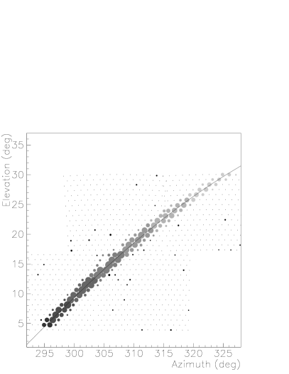
Figure 1: A 50 EeV (1 EeV = $10^{18}$ eV) UHECR event, as seen on the mirrors/PMTs of the detector (left) and in a time vs (SDP) angle plot (right). In the mirror/PMT display dots represent inactive tubes, circles represent active tubes where the size of the tube is proportional to the signal. Shaded tubes are included in the fit, with the shading representing the relative times: light to dark, early to late. In the time vs angle plot, the time is shown in units of 100 ns. The three fits are from Eq 1 with $\psi=180^{\circ}$ (light grey), $\psi=90^{\circ}$ (dark grey) the best fit $\psi$ (black).

4.2 Calibration

Once the geometry of the EAS is determined, one can use the photoelectron (NPE) signal of the PMTs to determine the number of charged particles, $N_{e}$, in the shower. In making this ${\rm NPE}\rightarrow N_{e}$ conversion, two important calibration issues come into play: the gains of the PMTs, and the atmospheric transparency to light. PMT gains are monitored nightly and monthly using a Xenon flash lamp and YAG laser. The atmosphere is monitored using a bistatic LIDAR system.

4.3 Fitting Profiles and Determining Energy

The HiRes-II analysis combines the PE signal from all the tubes in a given time bin, and converts this into a given number of charged particles in the EAS at a given depth in the atmosphere (measured in g/cm²). This conversion is strongly dependent on the geometry. One can estimate the energy of a shower from the number of charged particles, the amount of material traversed, and the average energy deposited per particle:

$$E_{0}=2.19{\rm\ MeV/(g/cm^{2})}\int^{\infty}_{0}N_{e}(X)dX$$ (2)

Since one often does not see the entire EAS, one must assume some profile of the number of charged particles for the unobserved part of the shower. We use the Gaisser-Hillas parameterization

$$N_{e}(X)=N_{\rm max}\left(\frac{X-X_{0}}{X_{\rm max}-X_{0}}\right)^{\frac{X_{\rm max}-X_{0}}{\lambda}}\exp\left(\frac{X-X_{\rm max}}{\lambda}\right)$$ (3)

where $X_{\rm max}$ is the depth at the maximum extent of the EAS, $N_{\rm max}$ is the number of particles at that depth, $X_{0}$ corresponds to the depth of the first interaction, and $\lambda$ is the interaction length. We fitted the observed portion of the shower to determine $X_{\rm max}$ and $N_{\rm max}$, holding $X_{0}=-60$ g/cm² (which is not physical, but gives the best fits when applied to simulations using CORSIKA[11]) and $\lambda=70$ g/cm².

Some of the observed light comes from the beam of Čerenkov light generated by the EAS and scattered into the detector. This light is subtracted from the signal in an iterative procedure. The photoelectron signal as a function of time and the calculated $N_{e}$ as a function of depth for the same 50 EeV event are shown in Fig. 2.

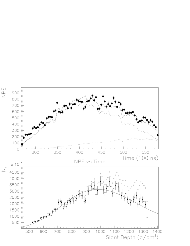
Figure 2: NPE and $N_{e}$ profiles in the 50 EeV event of Fig. fig:mirror-tvsa. In the the upper plot, points with error bars show the photoelectron signal (NPE) from all tubes included within a given time bin. The dashed and doted lines show calculations for the fluorescence and Čerenkov components of the signal, respectively, for this event at the best fit values of $X_{\rm max}$ and $N_{\rm max}$; the solid line shows the sum of the components. In the lower plot, filled points with error bars show the calculated $N_{e}$ extracted from the NPE signal as a function of depth in the atmosphere. The open points without error bars show the result of the calculation without subtracting off the Čerenkov component.

The energy is calculated from the HiRes-I signals in a similar way, except that the expected number of PE for a given shower is compared with the observed value. In other words, the fit is done using the number of PE at the detector rather than the extracted number of charged particles in the shower. The comparison is also done on a tube-by-tube basis rather than in time bins.

4.4 Event Selection

After events are reconstructed, one must select the sample from which to calculate the flux. This sample should be as large as possible and contain only well reconstructed events. The criteria used to make this selection are listed in Table 4.4.

Cuts used in HiRes-I and HiRes-II monocular analysis flux calculations. HiRes-I HiRes-II Minimum distance (Ang. Vel.) 5 km 1.5 km Minimum track length 8^∘ 10^∘        in ring 1 only 7^∘ Range of tubes per degree [0.85,3] [0.85,3] Minimum NPE per degree 25 25 Maximum zenith angle 60^∘ Minimum depth seen 150 g/cm² Minimum extent seen 150 g/cm² $X_{\rm max}$ observed required Maximum Čerenkov correction 60% Profile contraint converges required Data period starting 6/1997 12/1999 Data period ending 9/2001 5/2000

5 Monte Carlo Simulation

To determine the flux of UHECR, one needs to know the aperture over which the UHECRs are collected. This aperture varies with energy and must be determined through Monte Carlo (MC) simulation. However, one can also use MC simulation to check that one understands the data and its reconstruction in the detector. Extensive comparisons of distributions in data and in simulated samples of events provides confidence that the calculated aperture is correct.

The details of MC event generation have been published elsewhere.[10] It is clear, however, that one needs to model the details of the trigger, the extra tube distribution, and the transmission of light in the atmosphere to sufficient accuracy to obtain good agreement between data and MC.

I will show four comparisons between data and MC, all taken from the HiRes-II analysis. The first, in Fig. 3, shows the distribution of observed light (NPE) divided by the track length. The light distribution is sensitive to the yield, trigger, and geometry, among other things. The second and third comparisons, also in Fig. 3, show the distributions of $R_{p}$ and $\psi$. The good agreement gives us confidence in our calculation of the aperture. Finally, there is the energy distribution in Fig 4, which enters directly into the calculation of the flux. Note that the energy distribution has a binning such that there are no bins with less than two events. The HiRes-II aperture, with the same binning, is shown in Fig. 5.

Figure 3: Comparisons of the number of photoelectrons (NPE) per degree of track (left) and the EAS geometry variables $R_{p}$ and $\psi$ (right) between data (points) and MC (histogram) where in each case the MC distribution has been normalized to have the same area as the data. The bottom plots show the ratio of the two above distributions: data/MC.

Figure 4: A comparison of the reconstructed energy between data (points) and MC (histogram), where the MC distribution has been normalized to have the same area as the data. The bottom plot shows the ratio of the two distributions: data/MC. The vertical scale is number of events per 0.1 decade of energy.

Figure 5: The HiRes-II aperture as calculated in the MC.

6 Flux

With the event samples in hand, and confidence in our calculated aperture, we can extract the flux. Fig. 6, shows the calculated flux from HiRes-I (triangles) and HiRes-II (circles). The fluxes have been multiplied by $E^{3}$ in order to emphasize changes in the spectral index.

Figure 6: The UHECR flux, multiplied by $E^{3}$, as measured by HiRes-I (triangles) and HiRes-II (circles). The solid line is a two component fit to the data consisting of a galactic (dotted line) and extragalactic (dashed line) spectrum. The extragalactic sources evolve as $(1+z)^{m}$ with $m=3$ and have a distribution modified by the observed density of galaxies.

To evaluate the significance of these spectra, I have fitted the measured points to an astrophysical model of the sources and propagation of UHECRs. In choosing this model, I have been motivated by Occam’s Razor, sticking with known physical processes, and assuming only that the extragalactic sources of UHECR are distributed throughout the universe, and evolve in their density in the same way as the luminous matter in galaxies. To this is added a phenomenologically motivated galactic spectrum at lower energies.

The extragalactic spectrum is assumed to consist of protons, and have a power law spectrum at the source, with a fitted spectral slope parameter. This spectrum is modified by energy losses as the UHECRs traverse the intra-galactic medium. The energy loss formalism is taken from the work of Berezinsky et al.[12, 13] The sources are taken to be uniformly distributed out to a red-shift of $z=4$, with a density at any given $z$ modified by the observed density of galaxies at that red-shift[14, 15] and evolving as $(1+z)^{m}$ with $m=3$ (which is the best fit value and approximately the same as the observed stellar formation rate[16]). Using $m=0$, increases the $\chi^{2}$ of the fit by 3.5 while not accounting for the observed density of galaxies increases the $\chi^{2}$ by 1.5.

The galactic component of the spectrum is assumed to consist of iron nuclei. Motivation for this assumption comes from the Fly’s Eye composition measurement,[17] which shows an approximately linear (in $\log E$) change from a heavy composition (iron) to a light one (protons). The spectral form is assumed to be $E^{-3}$, consistent with the UHECR spectrum below $10^{17}$ eV, multiplied by a linear (in $\log E$) factor going from unity at $10^{17}$ eV, to zero at $10^{19.5}$ eV.

The fact that this model fits the data so well is due to agreement in its three features. First, the model clearly has a drastic reduction in flux above the GZK energy, a reduction which is also observed in the data, but with not as yet overwhelming statistical significance. More strongly constrained by observation are the “second knee” and “ankle”, which in this model are the result of electron pair production.[12, 13] The strength of the astrophysical source model is that it fits both the electron pair-production features and the pion production feature (the GZK cutoff) in the spectrum.

7 Conclusion

HiRes has recently announced preliminary measurements of the UHECR energy spectrum using each of its two detectors in monocular mode. We have fitted this spectrum to a two-component model of the UHECR sources, the extragalactic component of which conforms to the expectation of a nearly unform distribution of sources, modified by the observed distribution of luminous matter and its evolution as a function of red-shift. This model fits all the recognized features of the UHECR spectrum, not just the GZK cutoff.

Much has been made of the discrepancies between HiRes and AGASA, with AGASA seeing no evidence for the GZK cutoff, and HiRes being consistent with its presence. However, at energies below the GZK cutoff, the two experiments agree nicely in the shape of the spectrum, with only an offset in the flux, which can be attributed to a difference in energy scale within the stated systematic uncertainty of either experiment.[18]

References

References

- [1] A.M. Hillas, Ann. Rev. Astron. Astrophys. 22, 425 (1984).
- [2] K. Greisen, Phys. Rev. Lett. 16, 748 (1966).
- [3] G. T. Zatsepin and V. A. Kuzmin, Pis’ma Zh. Eksp. Teor. Fiz. 4, 114 (1966) [JETP Lett. 4, 78 (1966)].
- [4] N. Sakaki for the AGASA Collaboration, Proc. of 27th Int. Cosmic Ray Conf. (Hamburg) 1, 333 (2001).
- [5] From the AGASA website www-akeno.icrr.u-tokyo.ac.jp/AGASA as of July 2002.
- [6] R.M. Baltrusaitis et al. Nucl. Inst. Meth. A 240, 410 (1985).
- [7] D. J. Bird et al., Phys. Rev. Lett. 71, 3401 (1993)
- [8] Pierre Auger Observatory, Design Report.
- [9] T. Abu-Zayyad et al., astro-ph/0208243.
- [10] T. Abu-Zayyad et al., astro-ph/0208301.
-
[11]
D. Heck et al., FZKA 6019 (1998),
Forschungszentrum Karlsruhe;
http://www-ik3.fzk.de/heck/corsika/physics_description/corsika_phys.html. - [12] V.S. Berezinksy, S.I. Grigorieva, Astron. Astroph. 199, 1 (1988).
- [13] V. Berezinsky, A.Z. Gazizov, S.I. Grigorieva, hep-ph/9294357.
- [14] M. Blanton, P. Blasi, A.V. Olinto, Astropart. Phys., 15, 275 (2001).
- [15] Saunders et al., Mon. Not. R. Astron. Soc. 317, 55 (2000).
- [16] S.J. Lilly et al., Astrophys. J. 460, L1.
- [17] D.J. Bird et al., Astrophys. J. 441, 144 (1995).
- [18] D.R. Bergman, Proceedings of ICHEP 2002, 106 (2003); also see http://www.ichep02.nl/Transparencies/PAC/PAC-1/PAC-1-2.Bergman.pdf.