Partial Wave Analyses of $J/\psi\to\gamma K^{+}K^{-}$ and $\gamma K^{0}_{S}K^{0}_{S}$

Abstract

Results are presented on $J/\psi$ radiative decays to $K^{+}K^{-}$ and $K^{0}_{S}K^{0}_{S}$ based on a sample of 58M $J/\psi$ events taken with the BES II detector. A partial wave analysis is carried out using the relativistic covariant tensor amplitude method in the 1-2 GeV mass range. There is conspicuous production due to the $f^{\prime}_{2}(1525)$ and $f_{0}(1710)$. The latter peaks at a mass of $1740\pm 4^{+10}_{-25}$ MeV with a width of $166{{}^{+5}_{-8}}{{}^{+15}_{-10}}$ MeV. Spin 0 is strongly preferred over spin 2. For the $f^{\prime}_{2}(1525)$, the helicity amplitude ratios are determined to be $x^{2}=1.00\pm 0.28^{+1.06}_{-0.36}$ and $y^{2}=0.44\pm{0.08}^{+0.10}_{-0.56}$.

I Introduction

QCD predicts the existence of glueballs, the bound states of gluons, and the observation of glueballs is, to some extent, a direct test of QCD. Such gluonic states are expected to give rise to a rich isoscalar meson spectroscopy, and Lattice Gauge Theory calculations predict, in particular, that the lowest-lying state should occur in the mass range 1.4-1.8 GeV and have $J^{PC}=0^{++}$ QCDL . For a $J/\psi$ radiative decay to two pseudoscalar mesons, only $J^{PC}$ values in the series $0^{++},~{}2^{++},~{}...$ are possible, so such states provide a very clean laboratory to search for the lowest mass scalar glueball.

There has been a long history of uncertainty about the properties of the $f_{0}(1710)$, one of the earliest glueball candidates. This history is reviewed in detail in the latest issue of the Particle Data Group (PDG) PDG and will not be repeated here. The latest analysis of Mark III data by Dunwoodie WMD favors $J^{P}=0^{+}$ over an earlier assignment of $2^{+}$, while the latest central production data of WA76 and WA102 also favor $0^{+}$ WA76 ; WA102 . In this paper, we present new results on $J/\psi\to\gamma K^{+}K^{-}$ and $\gamma K^{0}_{S}K^{0}_{S}$ based on a sample of 58M $J/\psi$ events taken with the upgraded Beijing Spectrometer (BES II) located at the Beijing Electron Positron Collider (BEPC).

II Bes detector

BES II is a large solid-angle magnetic spectrometer that is described in detail in Ref. BESII . Charged particle momenta are determined with a resolution of $\sigma_{p}/p=1.78\%\sqrt{1+p^{2}(\mbox{GeV}^{2})}$ in a 40-layer cylindrical drift chamber. Particle identification is accomplished by specific ionization ($dE/dx$) measurements in the drift chamber and time-of-flight (TOF) measurements in a barrel-like array of 48 scintillation counters. The $dE/dx$ resolution is $\sigma_{dE/dx}=8.0\%$; the TOF resolution is $\sigma_{TOF}=180$ ps for Bhabha events. Outside of the time-of-flight counters is a 12-radiation-length barrel shower counter (BSC) comprised of gas proportional tubes interleaved with lead sheets. The BSC measures the energies and directions of photons with resolutions of $\sigma_{E}/E\simeq 21\%/\sqrt{E(\mbox{GeV})}$, $\sigma_{\phi}=7.9$ mrad, and $\sigma_{z}$ = 2.3 cm. The iron flux return of the magnet is instrumented with three double layers of counters that are used to identify muons. The average luminosity of the BEPC accelerator is $4.0\times 10^{30}$ cm^-2$s^{-1}$ at the center-of-mass energy of 3.1 GeV.

In this analysis, a GEANT3 based Monte Carlo simulation package (SIMBES) with detailed consideration of real detector performance (such as dead electronic channels) is used. The consistency between data and Monte Carlo has been carefully checked in many high purity physics channels, and the agreement is quite reasonable.

III Event selection

The first level of event selection requires two charged tracks with total charge zero for $\gamma K^{+}K^{-}$ candidate events, and requires two positively-charged and two negatively-charged tracks for $\gamma K^{0}_{S}K^{0}_{S}$ events. These tracks are required to lie well within the acceptance of the detector and to have a good helix fit. More than one photon per event is allowed because of the possibility of fake photons coming from the interactions of charged tracks with the shower counter or from electronic noise in the shower counter.

For $J/\psi\to\gamma K^{+}K^{-}$, the vertex is required to lie within 2 cm of the beam axis ($x-y$ plane) and within 20 cm of the center of the interaction region (along $z$). Each of the charged particles is required to not register hits in the muon counters in order to remove $\gamma\mu^{+}\mu^{-}$ events. The following selection criteria are used to remove the large backgrounds from Bhabha events: (i) The opening angle of the two tracks satisfies $\theta_{op}<175^{\circ}$. (ii) The energy deposit of each track in BSC satisfies $E_{SC}<1.0$ GeV. In order to reduce the background from final states with pions and electrons, each event is required to have at least one kaon identified by the TOF. Requirements on two variables, $U$ and $P^{2}_{t\gamma}$, are imposed THimel . A “missing-neutral-energy” variable $U=(E_{miss}-|\stackrel{{\scriptstyle\rightarrow}}{{P}}_{miss}|)$ is required to satisfy $-0.10<U<0.20$ GeV; here $E_{miss}$ and $\stackrel{{\scriptstyle\rightarrow}}{{P}}_{miss}$ are the missing energy and momentum of all charged particles respectively. Also a “missing-$p_{t}$” variable $P^{2}_{t\gamma}$ = $4|\stackrel{{\scriptstyle\rightarrow}}{{P}}_{miss}|^{2}\sin^{2}{{\theta_{\gamma}}/2}$ is required to be $<0.002$ GeV², where $\theta_{\gamma}$ is the angle between the missing momentum and the photon direction. The $U$ cut removes most background from events having multipion or other neutral particles, such as $\rho\pi,~{}\gamma\pi^{+}\pi^{-}$ events; $P^{2}_{t\gamma}$ is used to eliminate background photons. The selection criteria for a good photon used here are based on those applied in previous BES I analyses JINS . In brief, the good photon is required to be isolated from the two charged tracks and to come from the interaction point.

In order to reduce the $J/\psi\to\pi^{0}K^{+}K^{-}$ and $J/\psi\to\pi^{0}\pi^{+}\pi^{-}$ contamination, all events surviving the above criteria which have two or more photons are kinematically fitted to these hypotheses. Those events with a fit $\chi^{2}<50$, and with photon pair invariant mass within 50 MeV$/c^{2}$ of the $\pi^{0}$ mass, are rejected. Finally, the two charged tracks and photon in the event are 4-C kinematically fitted to obtain better mass resolution and to suppress backgrounds further by the requirements $\chi^{2}_{\gamma K^{+}K^{-}}<10$ and $\chi^{2}_{\gamma K^{+}K^{-}}<\chi^{2}_{\gamma\pi^{+}\pi^{-}}$.

For $J/\psi\to\gamma K^{0}_{S}K^{0}_{S}$, the $K^{0}_{S}$ mesons in the event are identified through the decay $K^{0}_{S}\to\pi^{+}\pi^{-}$. The four charged tracks can be grouped into two pairs, each having two oppositely charged tracks with an acceptable distance of closest approach. Signal events are required to satisfy $\delta^{2}_{K_{S}}<(20\mbox{MeV}/c^{2})^{2}$, where $\delta^{2}_{K_{S}}=(M_{\pi^{+}\pi^{-}}(1)-M_{K_{S}})^{2}+(M_{\pi^{+}\pi^{-}}(2)-M_{K_{S}})^{2}$ and $M_{\pi^{+}\pi^{-}}$ is calculated at the $K^{0}_{S}$ decay vertex. The main backgrounds from $\gamma K^{0}_{S}K^{\pm}\pi^{\mp}$ and $\gamma K^{0}_{S}K^{0}_{S}\pi^{0}$ events are suppressed by requiring $U<0.10$ GeV, $P^{2}_{t\gamma}<0.005$ GeV² and the 4-C kinematic fit $\chi^{2}_{\gamma 4\pi}<10$.

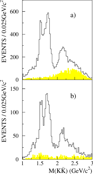
Figure 1: Invariant mass spectra of a) $K^{+}K^{-}$, b) $K^{0}_{S}K^{0}_{S}$ for $J/\psi\to\gamma K\bar{K}$ events, where the shaded histograms correspond to the estimated background contributions.

Fig. 1 shows the $K^{+}K^{-}$ and $K^{0}_{S}K^{0}_{S}$ mass spectra for the selected events, together with the corresponding background distributions. These two mass spectra agree closely below 2.0 GeV. The resonant structures in the mass regions of the $f^{\prime}_{2}(1525)$ and the $f_{0}(1710)$ are very clearly visible in both decay modes. Averaged over the whole mass range, the detection efficiency for $\gamma K^{+}K^{-}$ is $14.7\%$ and for $\gamma K^{0}_{S}K^{0}_{S}$ is $14.5\%$. For the $\gamma K^{+}K^{-}$ channel, the experimental background arises mainly from the non-resonant $K^{+}K^{-}\pi^{0}$ and two-body $K^{*\pm}K^{\mp}$ events which are peaked at high $K^{+}K^{-}$ masses. In the entire mass range, 14597 $\gamma K^{+}K^{-}$ events are reconstructed, and the detailed Monte Carlo simulation of the BES detector estimates a background of 3094 events. The estimation of the background events in the $\gamma K^{0}_{S}K^{0}_{S}$ sample is obtained from the $\delta^{2}_{K_{S}}$ side band $(28.7\mbox{MeV}/c^{2})^{2}<\delta^{2}_{K_{S}}<(35\mbox{MeV}/c^{2})^{2}$; this equal-area-selection provides a properly normalized background estimation. In Fig. 1b), there are 3169 selected $\gamma K^{0}_{S}K^{0}_{S}$ events and 413 background events.

IV Analysis results

We have carried out partial wave analyses using relativistic covariant tensor amplitudes constructed from Lorentz-invariant combinations of the 4-vectors and the photon polarization for $J/\psi$ initial states with helicity $\pm 1$ GZJ . Cross sections are summed over photon polarizations. The relative magnitudes and phases of the amplitudes are determined by a maximum likelihood fit. The background events obtained from Monte Carlo simulation or $\delta^{2}_{K_{S}}$ side band are included into the data samples, but with the opposite sign of log likelihood compared to data. These events cancel background within the data samples. These analyses are confined to masses less than 2 GeV in order to ensure that a description containing only $0^{++}$ and $2^{++}$ amplitudes be appropriate. The mass distributions of $K^{+}K^{-}$ and $K^{0}_{S}K^{0}_{S}$ after acceptance and isospin corrections for missing $\gamma K^{0}_{L}K^{0}_{L}$ and $\gamma K^{0}_{S}K^{0}_{S}$ with $K^{0}_{S}\to\pi^{0}\pi^{0}$ decays are shown in Fig. 2. The event topologies of the $K^{+}K^{-}$ and $K^{0}_{S}K^{0}_{S}$ modes are different, so that acceptance and background effects are rather different also; nevertheless, there is good quantitative agreement between the two distributions.

Figure 2: The mass distributions of $K\bar{K}$ from $J/\psi$ radiative decays, after acceptance and isospin corrections for missing $\gamma K^{0}_{L}K^{0}_{L}$ and $\gamma K^{0}_{S}K^{0}_{S}$ with $K^{0}_{S}\to\pi^{0}\pi^{0}$ decays.

IV.1 Bin-by-bin analysis

In the bin-by-bin analysis, the data in mass intervals 40 MeV wide are fitted with four helicity amplitudes, one for $J^{P}=0^{+}$ and three for $2^{+}$ amplitudes WMD . The mass interval width is chosen as a compromise between the desire for high statistics in each mass interval, and the need for detailed information on the mass dependence of each measured amplitude. In each mass interval, the $\gamma K\bar{K}$ data sample is analyzed in terms of the joint production and decay angular distribution of the pseudoscalar meson system. The S- and D-wave intensity distributions, $|a_{0,0}|^{2}$, $|a_{2,0}|^{2}$, $|a_{2,1}|^{2}$ and $|a_{2,2}|^{2}$ for $\gamma K\bar{K}$ data resulting from this bin-by-bin fit are shown as a function of mass in Fig. 3.

Figure 3: The mass dependence of the amplitude intensities for $\gamma K\bar{K}$ data. The solid curves correspond to the coherent superposition of the Breit-Wigner resonances fitted to the acceptance- and isospin-corrected data points obtained from the bin-by-bin fit. The dashed line histograms are the results of the global fit described in the text.

The $K\bar{K}$ S-wave intensity dominates the 1.7 GeV region. The solid curves in Fig. 3 correspond to fits of coherent superpositions of individual Breit-Wigner resonances to the data points of each intensity distribution. The following channels are considered:

$$J/\psi \to \gamma f^{\prime}_{2}(1525)$$

$$\to \gamma f_{0}(1710)$$

$$\to \gamma f_{2}(1270)$$

$$\to \gamma f_{0}(1500)$$

$$\to \gamma+{\rm broad~{}}0^{++}{\rm~{}and~{}}2^{++}{\rm~{}components}$$

The first two are dominant. There is evidence for existence of the $f_{2}(1270)$, and the $f_{0}(1500)$ is included here for consistency with the global fit below.

For the spin 0 amplitude, two interfering resonances ($f_{0}(1500$, $f_{0}(1710)$) and an interfering constant amplitude term, which is used to describe the broad S- wave contribution, are included. The mass and width of the $f_{0}(1500)$ are fixed to the PDG values; those of the $f_{0}(1710)$ are to be determined. The $f_{0}(1710)$ is well described by a Breit-Wigner of mass and width M $=1722\pm 17$ MeV, $\Gamma=167^{+37}_{-29}$ MeV, and the branching fraction for $J/\psi$ radiative decay to the combined $K\bar{K}$ modes is ${\cal B}(J/\psi\to\gamma f_{0}(1710)\to\gamma K\bar{K})=(11.1^{+1.7}_{-1.2})\times 10^{-4}$. The errors here are statistical errors.

For the spin 2 amplitudes, the $f^{\prime}_{2}(1525)$ and $f_{2}(1270)$ are included. There is also some $2^{++}$ structure above 2.0 GeV in $K\bar{K}$ mass, which could contribute to the present fitted range, and thus the tail of a high mass $2^{++}$ state is included in our fit. We choose a resonance mass of 2250 MeV and width of 350 MeV to represent the structure in the higher mass region. The mass and width of the $f_{2}(1270)$ are fixed at the values quoted in the PDG. For the tensor resonance, $f^{\prime}_{2}(1525)$, its mass and width are fixed to the values M = 1519 MeV, $\Gamma=75$ MeV determined by the global fit which is described below, and the total branching fraction and ratios of amplitude intensities are determined to be ${\cal B}(J/\psi\to\gamma f^{\prime}_{2}(1525)\to\gamma K\bar{K})=(4.02\pm 0.51)\times 10^{-4}$; $x^{2}\equiv{\displaystyle{{|a_{2,1}|^{2}}/{|a_{2,0}|^{2}}}}=1.32\pm 0.29$, $y^{2}\equiv{\displaystyle{{|a_{2,2}|^{2}}/{|a_{2,0}|^{2}}}}=0.38\pm 0.20$. The intensity of the $f_{2}(1270)$ is poorly measured because of the relatively low statistics and the weak coupling of this state to $K\bar{K}$. The amount of spin 2 component in the 1.7 GeV mass region is small, $\sim(16\pm 9)\%$. The errors shown above are statistical and are obtained from the Breit-Wigner fit.

IV.2 Global fit analysis

We now turn to the global fit to the $J/\psi\to\gamma K^{+}K^{-}$ and $J/\psi\to\gamma K^{0}_{S}K^{0}_{S}$ data. Each sample is analyzed independently, and the fit results shown below are for their averaged values. This fit has the merit of constraining phase variations as a function of mass to simple Breit-Wigner forms. It also performs the optimum averaging of helicity amplitudes and their phases over resonances. Partial waves are fitted to the data for the same components described in the bin-by-bin fit. The broad $0^{++}$ component improves the fit significantly; removing it causes the log likelihood value to become worse by 221. For the $f_{2}(1270)$ and $f_{0}(1500)$, we use PDG values of masses and widths, but allow the amplitudes to vary in the fit. For the $f_{2}^{\prime}(1525)$, relative phases are consistent with zero within experimental errors. It is expected theoretically that relative phases should be very small, on order of $\alpha\simeq 1/137$ for the electromagnetic transitions $J/\psi\to\gamma+2^{+}$. In view of the agreement with expectation, these relative phases are set to zero in the final fit, so as to constrain intensities further.

A free fit to $f_{2}^{\prime}(1525)$ gives a fitted mass of $1519\pm 2$ MeV and a width of $75\pm 4$ MeV. The fitted mass and width of the $f_{0}(1710)$ are M $=1740\pm 4$ MeV and $\Gamma=166^{+5}_{-8}$ MeV, respectively. The fitted intensities are illustrated in Fig. 4. For the $f_{2}^{\prime}(1525)$, we find the ratios of helicity amplitudes $x^{2}=1.00\pm 0.28$ and $y^{2}=0.44\pm 0.08$. In this fit, we allow some $0^{+}$ contribution under the $f_{2}^{\prime}(1525)$ peak, while previous analyses by DM2 and Mark III [10, 11] ignored the small $0^{+}$ contributions. The branching fractions of the $f^{\prime}_{2}(1525)$ and the $f_{0}(1710)$ determined by the global fit are ${\cal B}(J/\psi\to\gamma f^{\prime}_{2}(1525)\to\gamma K\bar{K})=(3.42\pm 0.15)\times 10^{-4}$ and ${\cal B}(J/\psi\to\gamma f_{0}(1710)\to\gamma K\bar{K})=(9.62\pm 0.29)\times 10^{-4}$ respectively. The errors shown here are also statistical. An alternative fit to $f_{J}(1710)$ with $J^{P}=2^{+}$ is worse by 258 in log likelihood relative to $0^{+}$ for $\gamma K^{+}K^{-}$ data and by 67 for $\gamma K^{0}_{S}K^{0}_{S}$. Remembering that three helicity amplitudes are fitted for spin 2 but only one for spin 0, the fit with $J^{P}=0^{+}$ is preferred by $>10\sigma$ after considering the two data samples together.

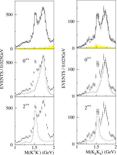
Figure 4: The $K\bar{K}$ invariant mass distributions from $J/\psi\to\gamma K^{+}K^{-}$ and $J/\psi\to\gamma K^{0}_{S}K^{0}_{S}$. The points are the data and the full histograms in the top panels show the maximum likelihood fit. Histograms on subsequent panels show the complete $0^{+}$ and $2^{+}$ contributions including all interferences.

The separation between spin 0 and 2 is illustrated in Fig. 5, taking the $J/\psi\to\gamma K^{+}K^{-}$ data as the example. Let us denote the polar angle of the kaon in the $K\bar{K}$ rest frame by $\theta_{K}$, and the polar angle of the photon in the $J/\psi$ rest frame by $\theta_{\gamma}$. The data are fitted simultaneously including important correlations between $\theta_{K}$ and $\theta_{\gamma}$. The left panels show resulting fits to $\cos\theta_{K}$ for $J=0$ and 2. There is no significant difference between the two fits. The distributions should be flat for $0^{+}$, but the interference with the tail of $f_{2}^{\prime}(1525)$ has a large effect. The right panels show the fits to $\cos\theta_{\gamma}$; the optimum fit is visibly better for $J=0$ than for $J=2$. [If one fits only the $\cos\theta_{\gamma}$ distribution, it is possible to fit equally well with $J=0$ or 2, but then the fit to $\cos\theta_{K}$ gets much worse.]

Figure 5: Projections in $\cos\theta_{K}$ and $\cos\theta_{\gamma}$ for $0^{++}$ and $2^{++}$ assumptions. The points are the data ($J/\psi\to\gamma K^{+}K^{-}$ sample), and the histograms are the global fit results.

If the $f_{0}(1500)$ is removed from the fit, the log likelihood is worse by 1.65 (3.58) for $K^{+}K^{-}$ ($K^{0}_{S}K^{0}_{S}$), corresponding to about 1.3$\sigma$ (2.2$\sigma$). If the $f_{2}(1270)$ is removed, the likelihood is worse by 57.5 (13.6) for $K^{+}K^{-}$ ($K^{0}_{S}K^{0}_{S}$), corresponding to $>5\sigma$ (3.8$\sigma$).

V Systematic error

The systematic error for the global fit is estimated by adding or removing small components used in the fit, replacing the $f_{0}(1500)$ with the $f_{0}(1429)$, $\Gamma=169$ MeV, described in Ref. WMD , varying the mass and width of the large $f^{\prime}_{2}(1525)$ within the PDG errors, varying the mass and width of $f_{0}(1710)$ based on the difference between the $K^{+}K^{-}$ and $K^{0}_{S}K^{0}_{S}$ decay modes, and varying the background component within reasonable limits in both the global fit and bin-by-bin fit. It also includes the uncertainty in the number of $J/\psi$ events analyzed and the difference from two different choices of MDC wire resolution simulation.

The uncertainty about the shape of broad $0^{++}$ background is included in the systematic error also. An incoherent fit with this broad component and a fit with alternative forms for the $s$-dependence using the parametrization of Zou and Bugg ZOU for the $f_{0}(400-1200)$ have been performed to estimate the systematic error from this source. This uncertainty affects the results significantly, especially the branching fractions, because of the interference between the broad structure and the other components. Therefore, the error from this model-dependence for the branching fraction measurements is separated from the statistical and other systematic errors in our final results. The systematic errors for the global fit are summarized in Table 1. For the mass and width, only the contributions from the model-dependence, which are large compared to the other errors, are shown in the table.

	M${}_{f^{\prime}_{2}(1525)}$	$\Gamma_{f^{\prime}_{2}(1525)}$	$x^{2}$	$y^{2}$	${\cal B}_{f^{\prime}_{2}(1525)}$	M${}_{f_{0}(1710)}$	$\Gamma_{f_{0}(1710)}$	${\cal B}_{f_{0}(1710)}$
remove $f_{0}(1500)$			${}^{+32}_{-0}$	${}^{+20}_{-0}$	$\pm 0$			${}^{+10}_{-0}$
use $f_{0}(1429)$			${}^{+0}_{-15}$	${}^{+0}_{-9}$	${}^{+0}_{-5}$			${}^{+3}_{-0}$
remove $f_{2}(1270)$			${}^{+42}_{-0}$	${}^{+0}_{-55}$	${}^{+6}_{-0}$			${}^{+0}_{-1}$
use the $\sigma$	$+0.66$	$+20$	${}^{+17}_{-9}$	${}^{+0}_{-14}$	${}^{+33}_{-0}$	$-1.44$	$+9$	${}^{+29}_{-0}$
incoherent $0^{++}$	$+0.99$	—	${}^{+6}_{-0}$	${}^{+0}_{-64}$	${}^{+45}_{-0}$	—	$+3$	${}^{+28}_{-0}$
M, $\Gamma$ of $f^{\prime}_{2}(1525)$			${}^{+49}_{-15}$	${}^{+0}_{-34}$	${}^{+11}_{-8}$			${}^{+4}_{-5}$
M, $\Gamma$ of $f_{0}(1710)$			${}^{+51}_{-17}$	${}^{+11}_{-36}$	$\pm 3$			${}^{+1}_{-0}$
M, $\Gamma$ of high $2^{++}$			${}^{+46}_{-14}$	${}^{+0}_{-59}$	${}^{+1}_{-4}$			${}^{+6}_{-0}$
background			${}^{+46}_{-17}$	${}^{+0}_{-55}$	${}^{+0}_{-3}$			${}^{+9}_{-10}$
$\delta_{N_{J/\psi}}$			—	—	$\pm 4.7$			$\pm 4.7$
wire resolution			—	—	$\pm 15$			$\pm 15$

Table 1: Estimation of systematic error (%) in the global fit. ${\cal B}_{f^{\prime}_{2}(1525)}$ and ${\cal B}_{f_{0}(1710)}$ are the branching fractions for $f^{\prime}_{2}(1525)$ and $f_{0}(1710)$ respectively.

VI Results and Discussion

The results of the bin-by-bin and global fits are summarized in Tables 2 and 3 respectively. For the bin-by-bin fit, the errors are statistical ones only, and for the global fit, the first error listed is the statistical error, the second error is the systematic error, and the third one for the branching fractions is for the model-dependence of the broad components.

	$f^{\prime}_{2}(1525)$	$f_{0}(1710)$
M (MeV)	1519 (fixed)	$1722\pm 17$
$\Gamma$ (MeV)	75 (fixed)	$167{{}^{+37}_{-29}}$
${\cal B}(J/\psi\to\gamma X,$
$X\to K\bar{K})(\times 10^{-4})$	$4.02\pm 0.51$	$11.1^{+1.7}_{-1.2}$
$x^{2}={\displaystyle{{|a_{2,1}|^{2}}/{|a_{2,0}|^{2}}}}$	$1.32\pm 0.29$	—–
$y^{2}={\displaystyle{{|a_{2,2}|^{2}}/{|a_{2,0}|^{2}}}}$	$0.38\pm 0.20$	—–

Table 2: Measurements of the $f^{\prime}_{2}(1525)$ and $f_{0}(1710)$ for the bin-by-bin fit. Errors shown are statistical only.

	$f^{\prime}_{2}(1525)$	$f_{0}(1710)$
M (MeV)	$1519\pm 2{{}^{+15}_{-5}}$	$1740\pm 4{{}^{+10}_{-25}}$
$\Gamma$ (MeV)	$75\pm 4{{}^{+15}_{-5}}$	$166{{}^{+5}_{-8}}{{}^{+15}_{-10}}$
${\cal B}(J/\psi\to\gamma X,$
$X\to K\bar{K})(\times 10^{-4})$	$3.42\pm 0.15{{}^{+0.69}_{-0.65}}{{}^{+1.55}_{-0.00}}$	$9.62\pm 0.29{{}^{+2.11}_{-1.86}}{{}^{+2.81}_{-0.00}}$
amp. ratios $x^{2}$	$1.00\pm 0.28{{}^{+1.06}_{-0.36}}$	—–
$y^{2}$	$0.44\pm 0.08{{}^{+0.10}_{-0.56}}$	—–

Table 3: Measurements of the $f^{\prime}_{2}(1525)$ and $f_{0}(1710)$ for the global fit. The first error is statistical, the second is systematic, and the third is that corresponding to model-dependence of the broad components.

The two fit methods, bin-by-bin and global, are based on different analysis concepts. In the bin-by-bin fit, the S- and D-wave intensities are fairly well determined and nearly model independent. The only model dependence in the bin-by-bin fit is the assumption that only S- and D-waves need be considered; this is reasonable, since one would not expect significant $4^{++}$ amplitudes below 2 GeV. However, due to limited statistics for each bin and the limited solid angle coverage of the detector, the relative phases of partial waves cannot be well determined. This causes larger uncertainties when extracting the mass and width of resonances by fitting only the partial wave intensities without the constraints of the relative phases between them. In the global fit, the phase variations as a function of mass are constrained to simple Breit-Wigner (BW) forms . The stability of the minimum optimizing procedure and statistical errors are better than those of the bin-by-bin fit. However, if some non-BW resonance is assumed to be a BW-form amplitude, this will give a model-dependent biased result. The model independent bin-by-bin result for the partial wave intensities can provide guidance for choosing components for the global fit. The final full amplitudes from the global fit definitely give a better fit to the whole set of data than the amplitudes obtained from fitting the partial wave intensities without constraints of relative phases between them.

Fortunately from Tables 2 and 3 and the comparison shown in Fig. 3, we see that the results obtained from the bin-by-bin fit and the global fit for the $f^{\prime}_{2}(1525)$ and $f_{0}(1710)$ agree with each other well within the errors. The ratios of the helicity amplitudes of the $f^{\prime}_{2}(1525)$ from the present analysis are in reasonable agreement with Krammer’s predictions krammer . These ratios provide useful information for testing models of the resonance production and decay mechanisms. Most importantly, the analysis demonstrates that the mass region around 1.7 GeV is predominantly $0^{++}$ from the $f_{0}(1710)$ 2pp ; this conclusion is consistent with that of references [3-5].

VII Summary

In summary, the partial wave analyses of $J/\psi\to\gamma K^{+}K^{-}$ and $J/\psi\to\gamma K^{0}_{S}K^{0}_{S}$ using 58M $J/\psi$ events of BES II show strong production of the $f^{\prime}_{2}(1525)$ and the S-wave resonance $f_{0}(1710)$. This confirms earlier conclusions that the spin-parity of the $f_{0}(1710)$ is $J^{P}=0^{+}$. The $f_{0}(1710)$ peaks at a mass of $1740\pm 4^{+10}_{-25}$ MeV with a width of $166{{}^{+5}_{-8}}{{}^{+15}_{-10}}$ MeV. For the $f^{\prime}_{2}(1525)$, the helicity amplitude ratios are determined to be $1.00\pm 0.28^{+1.06}_{-0.36}$ and $0.44\pm{0.08}^{+0.10}_{-0.56}$, respectively. They are consistent with theoretical predictions.

VIII Acknowledgments

The BES collaboration acknowledges the strong efforts of the BEPC staff and the helpful assistance we received from the members of the IHEP computing center. We also wish to thank William Dunwoodie and Walter Toki for useful discussions and suggestions. This work is supported in part by the National Natural Science Foundation of China under contracts Nos. 19991480,10225524,10225525, the Chinese Academy of Sciences under contract No. KJ 95T-03, the 100 Talents Program of CAS under Contract Nos. U-11, U-24, U-25, and the Knowledge Innovation Project of CAS under Contract Nos. U-602, U-34(IHEP); by the National Natural Science Foundation of China under Contract No.10175060(USTC); and by the Department of Energy under Contract No. DE-FG03-94ER40833 (U Hawaii). We wish to acknowledge financial support from the Royal Society for collaboration between the BES group and Queen Mary College, London.

References

(1) G. Bali, K. Schilling, A. Hulsebos, A. Irving, C.
Michael, and P. Stephenson, Phys. Rev. B309 (1993) 378;
C. Michael, Proceedings of Hadron 97, AIP
Conf. Series 432 (1997) 657;
W. Lee, and D. Weingarten, hep-lat/9805029;
C. Morningstar, and M. Peardon, Phys. Rev. D60
(1999) 034509.
(2) K. Hagiwara (Particle Data Group),
Phys. Rev. D66 (2002) 010001.
(3) W. Dunwoodie, Hadron Spectroscopy, AIP Conf. Series
432 (1997) 753.
(4) B. French , Phys. Lett. B214 (1999) 213.
(5) D. Barberis , Phys. Lett. B453 (1999) 305 and
316;
Phys. Lett. B462 (1999) 462.