Including gaussian uncertainty on the background estimate for upper limit calculations using Poissonian sampling

Abstract

A procedure to include the uncertainty on the background estimate for upper limit calculations using Poissonian sampling is presented for the case where a Gaussian assumption on the uncertainty can be made. Under that hypothesis an analytic expression of the likelihood is derived which can be written in terms of polynomials defined by recursion. This expression may lead to a significant speed up of computing applications that extract the upper limits using Toy Monte Carlo.

1 Introduction

In searches for rare processes where there is no statistical evidence of the signal, it is often convenient to combine the results of more independent selection channels in order to obtain the upper limit to the number of expected signal events. A statistical procedure using a likelihood ratio approach has been adopted to combine the results of the Higgs search done by the four LEP experiments ref:lep1  ref:lep2 . The likelihood ratio estimator $Q$ is defined as:

$$Q=\frac{{L}(s+b)}{{L}(b)}$$ (1)

where ${L}(s+b)$ and ${L}(b)$ are the likelihood functions in the hypotheses of the signal plus background and background only respectively.

In the case of a Poissonian sampling, only the number of events passing a number of independent selection channels is used as observable to discriminate the hypotheses of signal plus background versus background only. The likelihood functions ${L}(s+b)$ and ${L}(b)$ can be written, for the Poissonian sampling, as the product of Poisson probabilities:

$${L}(s+b) = \prod_{i=1}^{n_{ch}}\frac{e^{-(s_{i}+b_{i})}(s_{i}+b_{i})^{n_{i}}}{n_{i}!}$$ (2)

$${L}(b) = \prod_{i=1}^{n_{ch}}\frac{e^{-b_{i}}b_{i}^{n_{i}}}{n_{i}!}$$ (3)

where $n_{ch}$ is the number of selection channels, $s_{i}$ and $b_{i}$ are the expected number of signal and background events respectively and $n_{i}$ is the number of selected events. The following simplified expression for $Q$ is more convenient for computer computations:

$$Q=\frac{{L}(s+b)}{{L}(b)}=e^{-s_{tot}}\prod_{i=1}^{n_{ch}}\left(1+\frac{s_{i}}{b_{i}}\right)^{n_{i}}\,.$$ (4)

where $s_{tot}=\sum_{i=1}^{n_{ch}}s_{i}$.

In the case where $s$ is the number of produced events and $\epsilon_{i}$ are the efficiencies of each selection $s_{tot}=s\sum_{i=1}^{n_{ch}}\epsilon_{i}$. The absolute minimum of $-2\log(Q)$ as a function of $s$ gives the most likely value of the branching fraction. In case there is no evidence of the signal, it is possible to compute an upper limit at a given (usually 90% or 95%) Confidence Level (C.L.) using a Toy Monte Carlo, generating a large number of random experiments for different values of the signal $s$. The confidence level for the signal hypothesis can be computed as:

$$C.L._{s}=\frac{C.L._{s+b}}{C.L._{b}}=\frac{N_{Q_{s+b}\leq Q}}{N_{Q_{b}\leq Q}}$$ (5)

where $N_{Q_{s+b}\leq Q}$ and $N_{Q_{b}\leq Q}$ are the number of the generated experiments which have a likelihood ratio less then or equal to the measured one, in the background plus signal and background only hypothesis respectively.

Background uncertainty can be included in the definition of the likelihood applying a convolution with the distribution of the background, which is given by the assumed distribution of the background fluctuation. The case where the error on the background estimates $b_{i}$ can be assumed to be Poissonian has been studied in ref. ref:clpois . In other cases, the uncertainty may be better considered as Gaussian. This is true for instance when the background estimates are computed applying subtractions of different samples or applying scaling factors affected by gaussian uncertainties.

It should be remarked that the method applied in reference ref:clpois , which is also applied in this paper, does not have as good formal basis as it was originally thought. Reference ref:zech notes that the method is not correct from a frequentist point of view, nonetheless, it “seems to be acceptable to many pragmatic frequentists”. This caveat should be kept in mind when handling the results reported in the following.

2 Including Gaussian background uncertainties in the upper limit extraction

Under the assumption that the uncertainties are Gaussian, equations (2) and (3) need to be convolved with a Gaussian function, and become:

$${L}(s+b) = \prod_{i=1}^{n_{ch}}\int_{-\infty}^{+\infty}{\mathrm{d}}b_{i}^{\prime}\frac{1}{\sqrt{2\pi\sigma_{i}^{2}}}e^{-\frac{(b_{i}^{\prime}-b_{i})^{2}}{2\sigma_{i}^{2}}}\frac{e^{-(s_{i}+b_{i}^{\prime})}(s_{i}+b_{i}^{\prime})^{n_{i}}}{n_{i}!}$$ (6)

$${L}(b) = \prod_{i=1}^{n_{ch}}\int_{-\infty}^{+\infty}{\mathrm{d}}b_{i}^{\prime}\frac{1}{\sqrt{2\pi\sigma_{i}^{2}}}e^{-\frac{(b_{i}^{\prime}-b_{i})^{2}}{2\sigma_{i}^{2}}}\frac{e^{-b_{i}^{\prime}}(b_{i}^{\prime})^{n_{i}}}{n_{i}!}$$ (7)

where $\sigma_{i}$ is the error on the estimate of the background $b_{i}$. The integration can be extended from $-\infty$ to $+\infty$ including the unphysical negative signal region when the area of the tails of the Gaussian distributions in that region are negligible. This is true if $\sigma_{i}$ is sufficiently smaller than $b_{i}$. In that case, the integrals are easily manageable analytically. The integration can be performed exploiting the following expression for the exponent of the exponential term:

$$-\frac{(b_{i}^{\prime}-b_{i})^{2}}{2\sigma_{i}^{2}}-(s_{i}+b_{i}^{\prime})=-\frac{(b_{i}^{\prime}-b_{i}+\sigma_{i}^{2})^{2}}{2\sigma_{i}^{2}}-(s_{i}+b_{i})+\frac{\sigma_{i}^{2}}{2}$$ (8)

The intagration variable can be normalized to $z=(b_{i}^{\prime}-b_{i}+\sigma_{i}^{2})/\sigma_{i}$ so that the likelihood functions become:

$${L}(s+b) = \prod_{i=1}^{n_{ch}}\frac{1}{\sqrt{2\pi}}\frac{1}{n_{i}!}e^{-(s_{i}+b_{i})}e^{\sigma_{i}^{2}/2}\int_{-\infty}^{+\infty}e^{-z^{2}/2}(s_{i}+b_{i}-\sigma^{2}_{i}+\sigma_{i}z)^{n_{i}}{\mathrm{d}}z$$ (9)

$${L}(b) = \prod_{i=1}^{n_{ch}}\frac{1}{\sqrt{2\pi}}\frac{1}{n_{i}!}e^{-b_{i}}e^{\sigma_{i}^{2}/2}\int_{-\infty}^{+\infty}e^{-z^{2}/2}(b_{i}-\sigma^{2}_{i}+\sigma_{i}z)^{n_{i}}{\mathrm{d}}z$$ (10)

The integrals present in the likelihood functions are all of the form:

$$\int_{-\infty}^{+\infty}e^{-z^{2}/2}(\alpha+\beta z)^{n}{\mathrm{d}}z$$ (11)

and can be computed expanding the polynomial and using:

$$\int_{-\infty}^{+\infty}e^{-z^{2}/2}z^{2n}{\mathrm{d}}z = \sqrt{2\pi}\prod_{k=0}^{n}(2k+1)$$ (12)

$$\int_{-\infty}^{+\infty}e^{-z^{2}/2}z^{2n+1}{\mathrm{d}}z = 0$$ (13)

or can be alternatively computed defining the $n$-th degree polynomials:

$$p_{n}(\alpha,\beta)=\frac{1}{\sqrt{2\pi}}\int_{-\infty}^{+\infty}e^{-z^{2}/2}(\alpha+\beta z)^{n}{\mathrm{d}}z\,.$$ (14)

It can be easily shown that the polynomials satisfy the recursion relation:

$$p_{n}(\alpha,\beta)=\alpha p_{n-1}(\alpha,\beta)+(n-1)\beta^{2}p_{n-2}(\alpha,\beta)\,.$$ (15)

The first polynomials are:

$$p_{0}(\alpha,\beta) = 1$$

$$p_{1}(\alpha,\beta) = \alpha$$

$$p_{2}(\alpha,\beta) = \alpha^{2}+\beta^{2}$$

$$p_{3}(\alpha,\beta) = \alpha^{3}+3\alpha\beta^{2}$$

$$p_{4}(\alpha,\beta) = \alpha^{4}+6\alpha^{2}\beta^{2}+3\beta^{4}$$

$$p_{5}(\alpha,\beta) = \alpha^{5}+10\alpha^{3}\beta^{2}+15\alpha\beta^{4}$$

$$...$$

The likelihood functions can be rewritten as:

$${L}(s+b) = \prod_{i=1}^{n_{ch}}e^{-(s_{i}+b_{i}-\sigma_{i}^{2}/2)}\frac{p_{n_{i}}(s_{i}+b_{i}-\sigma^{2}_{i},\sigma_{i})}{n_{i}!}\,,$$ (16)

$${L}(b) = \prod_{i=1}^{n_{ch}}e^{-(b_{i}-\sigma_{i}^{2}/2)}\frac{p_{n_{i}}(b_{i}-\sigma^{2}_{i},\sigma_{i})}{n_{i}!}\,.$$ (17)

The computation of the upper limit with the Toy Monte Carlo can be performed with a small modification to the code used for the computation in the case of no error. The following simplified expression for $Q$ may be convenient:

$$Q=\frac{{L}(s+b)}{{L}(b)}=e^{-s_{tot}}\prod_{i=1}^{n_{ch}}\frac{p_{n_{i}}(s_{i}+b_{i}-\sigma_{i}^{2},\sigma_{i})}{p_{n_{i}}(b_{i}-\sigma_{i}^{2},\sigma_{i})}\,.$$ (18)

The usage of polynomials instead of other means of numerical integration provides a significant sepeed up of the code in computer calculations that use Toy Monte Carlo.

3 Application to the search for $B^{-}\rightarrow{\tau}^{-}\bar{\nu}$ in BABAR

The above method has been applyied in the search for $B^{-}\rightarrow{\tau}^{-}\bar{\nu}$ using in BABAR experiment ref:babar using the events where one $B$ meson is fully reconstructed, where the assumptions made in this paper hold. The search has shown no evidence for the signal. In order to evaluate the 90% C.L. limit on $B(B^{-}\rightarrow{\tau}^{-}\bar{\nu})$ , a large number of Toy Monte Carlo experiments have been generated for different values of the assumed branching fraction, each corresponding to an expected number of produced events $s$. Fig. 1 and. 2 show $-2\log(Q)$ and confidence level as a function of $B(B^{-}\rightarrow{\tau}^{-}\bar{\nu})$ with and without including the systematic error on the estimated background. The limit obtained including the uncertainty is less stringent than the limit obtained neglecting this effect.

4 Conclusion

A procedure to include Gaussian uncertainty on the background estimate for upper limit calculations using Poissonian sampling has been presented. The likelihood can be written in terms of polynominals that can be defined recursively. This approach makes computing calculation of confidence levels more efficient. The technique described in this paper has been applied in BABAR for to the search for $B^{-}\rightarrow{\tau}^{-}\bar{\nu}$ .

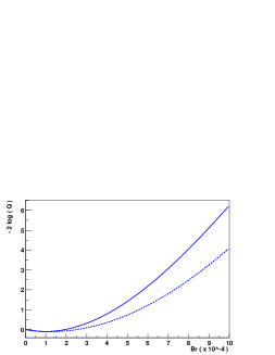
Figure 1: $-2\log(Q)$ as a function of $B(B^{-}\rightarrow{\tau}^{-}\bar{\nu})$ with (dashed) and without (solid) including the systematic error on the estimated background.

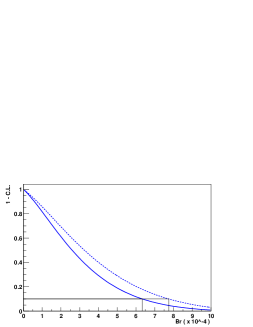
Figure 2: Confidence level as a function of $B(B^{-}\rightarrow{\tau}^{-}\bar{\nu})$ with (dashed) and without (solid) including the systematic error on the estimated background.

References

• (1) The LEP Working Group for Higgs Boson Searches, Lower bound for Standard Model Higgs boson mass from combining the results of the four LEP experiments, CERN-EP/98-046.
• (2) The LEP Working Group for Higgs Boson Searches, Limits for the Higgs boson masses from combining the data of the four LEP experiments at $\sqrt{s}\leq 183GeV$, CERN-EP/99-060.
• (3) K.K.Gan et al., Incorporation of the statistical uncertainty in the background estimate into the upper limit on the signal, N.I.M. A412 (1998) 475-482.
• (4) G.Zech, Frequentistic and Bayesian confidence limits, Eur.Phys.J.direct C4:12,2002.
• (5) B. Aubert, et al., BABAR Collaboration, A Search for $B^{-}\rightarrow\tau^{-}\bar{\nu}$ Recoiling Against a Fully Reconstructed $B$ presented to 2003 Rencontres de Moriond: Electroweak Interactions and Unified Theories hep-ex/0304030, BABAR-CONF-03/004, SLAC-PUB-9716
Refer to caption