First Evidence of $\Lambda\overline{\Lambda}$ in $\chi_{cJ}$ Decays

Abstract

The first observation of $\chi_{cJ}$ (J=0,1,2) decays to $\Lambda\overline{\Lambda}$ is reported using $\psi(2S)$ data collected with the BESII detector at the BEPC. The branching ratios are determined to be ${\cal B}(\chi_{c0}\rightarrow\Lambda\overline{\Lambda})=(4.7^{+1.3}_{-1.2}\pm 1.0)\times 10^{-4}$ , ${\cal B}(\chi_{c1}\rightarrow\Lambda\overline{\Lambda})=(2.6^{+1.0}_{-0.9}\pm 0.6)\times 10^{-4}$ and ${\cal B}(\chi_{c2}\rightarrow\Lambda\overline{\Lambda})=(3.3^{+1.5}_{-1.3}\pm 0.7)\times 10^{-4}$. Results are compared with model predictions.

I Introduction

It has been shown both in theoretical calculations and experimental measurements that the lowest Fock state expansion (color singlet mechanism, CSM) of charmonium states is insufficient to describe P-wave quarkonium decays. Instead, the next higher Fock state (color octet mechanism, COM) plays an important role so ; width . Our earlier measurement width of the total width of the $\chi_{c0}$ agrees rather well with the COM expectation. The calculation of the partial width of $\chi_{cJ}\rightarrow p\overline{p}$, by taking into account the COM of $\chi_{cJ}$ decays and using a carefully constructed nucleon wave function wong , obtains results in reasonable agreement with measurements pdg . The nucleon wave function was then generalized to other baryons, and the partial widths of many other baryon anti-baryon pairs predicted. Among these predictions, the partial width of $\chi_{cJ}\rightarrow\Lambda\overline{\Lambda}$ is about half of that of $\chi_{cJ}\rightarrow p\overline{p}$ (J=1,2) wong .

In this paper, we report on an analysis of the $\gamma\pi^{+}\pi^{-}p\overline{p}$ final state produced in $\psi(2S)$ decays. Evidence for the decays of $\chi_{cJ}$ to $\Lambda\overline{\Lambda}$ is observed for the first time. The data used for this analysis were taken with the Beijing Spectrometer detector (BESII) at the Beijing Electron Positron Collider (BEPC) at a center-of-mass (CM) energy corresponding to $M_{\psi(2S)}$. The data sample corresponds to a total of about 15 million $\psi(2S)$ decays.

BES is a conventional solenoidal magnet detector that is described in detail in Ref. bes ; BESII is the upgraded version of the BES detector bes2 . A 12-layer vertex chamber (VTC) surrounding the beam pipe provides trigger information. A forty-layer main drift chamber (MDC), located radially outside the VTC, provides trajectory and energy loss ($dE/dx$) information for charged tracks over $85\%$ of the total solid angle with a momentum resolution of $\sigma_{p}/p=0.0178\sqrt{1+p^{2}}$ ($p$ in $\hbox{\rm GeV}/c$) and a $dE/dx$ resolution for hadron tracks of $\sim 8\%$. An array of 48 scintillation counters surrounding the MDC measures the time-of-flight (TOF) of charged tracks with a resolution of $\sim 200$ ps for hadrons. Radially outside the TOF system is a 12 radiation length, lead-gas barrel shower counter (BSC). This measures the energies of electrons and photons over $\sim 80\%$ of the total solid angle with an energy resolution of $\sigma_{E}/E=21\%/\sqrt{E}$ ($E$ in GeV). Outside the solenoidal coil, which provides a 0.4 Tesla magnetic field over the tracking volume, is an iron flux return that is instrumented with three double layers of counters that identify muons of momentum greater than 0.5 GeV/c.

A Monte Carlo simulation is used for the determination of the mass resolution and detection efficiency, as well as the estimation of the background. For the signal channels, $\psi(2S)\rightarrow\gamma\chi_{cJ}$, $\chi_{cJ}\rightarrow\Lambda\overline{\Lambda}$, the angular distribution of the photon emitted in the $\psi(2S)$ decay is assumed to be that for a pure E1 transition. The $\Lambda$ in the $\chi_{cJ}$ CM system and the daughter particles in the $\Lambda$ CM system are generated isotropically. A total of 10000 events are generated for each $\chi_{cJ}$ state with $\Lambda\rightarrow\pi^{-}p$ and $\overline{\Lambda}\rightarrow\pi^{+}\overline{p}$. For the estimation of the number of $\psi(2S)$ events and the estimation of the systematic error, $\psi(2S)\rightarrow\pi^{+}\pi^{-}J/\psi$, $J/\psi\rightarrow p\overline{p}$ events are generated, where the $\pi^{+}\pi^{-}$ invariant mass is distributed as measured in Ref. bll .

The simulation of the detector response, including interactions of secondary particles in the detector material, uses a Geant3 based package SIMBES. Reasonable agreement between data and Monte Carlo simulation is observed in testing various channels, including $e^{+}e^{-}\rightarrow\gamma e^{+}e^{-}$ (Bhabha), $e^{+}e^{-}\rightarrow\mu^{+}\mu^{-}$, $J/\psi\rightarrow p\overline{p}$, and $\psi(2S)\rightarrow\pi^{+}\pi^{-}J/\psi$, $J/\psi\rightarrow\ell^{+}\ell^{-}$.

II Event selection

The analysis uses the same photon selection and charged particle identification (ID) criteria as were used in Ref. had . When selecting photons it is necessary to remove photons produced by hadronic interactions of charged tracks with the detector material. This is achieved by cutting on the angle between the neutral cluster and the charged track in the BSC. The number of photon candidates in an event is not limited.

Both TOF and $dE/dx$ information are used for charged particle identification. Probabilities of a track being a pion ($Prob_{\pi}$), kaon ($Prob_{K}$), or proton ($Prob_{p}$) are assigned to each charged track. For the decay channel of interest, the candidate events are required to satisfy the following selection criteria:

1. Each charged track is required to be well fit to a three-dimensional helix and be in the polar angle region $|\cos\theta_{MDC}|<0.8$.

2. The number of charged tracks is four with net charge zero.

3. The two lower momentum positive and negative charged tracks are assumed to be the $\pi^{+}$ and the $\pi^{-}$, and the other two tracks are regarded as the proton and the antiproton. Four-constraint kinematic fits to the decay hypothesis are performed with each of the photon candidates, and the one with the smallest $\chi^{2}$ is taken as the real photon. The $\chi^{2}$ probability of the fit is required to be greater than 1%.

4. The particle identification assignment of each charged track must satisfy $Prob_{\pi}$ (for $\pi^{\pm}$) or $Prob_{p}$ (for $p$ or $\overline{p}$) $>0.01$.

A four-constraint fit assuming $\psi(2S)\rightarrow\pi^{+}\pi^{-}p\overline{p}$ is also performed to select $\psi(2S)\rightarrow\Lambda\overline{\Lambda}$ and $\psi(2S)\rightarrow\pi^{+}\pi^{-}J/\psi,J/\psi\rightarrow p\overline{p}$ events for checking the reliability of the analysis of $\chi_{cJ}\rightarrow\Lambda\overline{\Lambda}$ and to calculate the total number of $\psi(2S)$ events. The selection criteria used are the same as for $\chi_{cJ}\rightarrow\Lambda\overline{\Lambda}$ except that no photon information is used.

III Event analysis

Fig. 1 shows a scatter plot of the $\pi^{+}\overline{p}$ versus the $\pi^{-}p$ invariant mass for events with $\pi^{+}\pi^{-}p\overline{p}$ mass between $3.38$ GeV/$c^{2}$ and $3.60$ GeV/$c^{2}$. The cluster of events in the lower left corner shows a clear $\Lambda\overline{\Lambda}$ signal.

Figure 1: Scatter plot of $\pi^{+}\overline{p}$ versus $\pi^{-}p$ invariant mass for selected $\gamma\pi^{+}\pi^{-}p\overline{p}$ events with the $\pi^{+}\pi^{-}p\overline{p}$ mass in the $\chi_{cJ}$ mass region.

Selecting events in $\chi_{cJ}$ mass region and requiring the mass of $\pi^{+}\overline{p}$ ($\pi^{-}p$) to be smaller than 1.15 GeV/$c^{2}$, the $\pi^{-}p$ ($\pi^{+}\overline{p}$) mass distribution shown in Fig. 2 is obtained. A clear $\Lambda$ signal can be seen, and the background below the peak is very small. A fit of the mass distribution gives $m_{\Lambda}=(1114.6\pm 0.6)~{}\hbox{MeV}/c^{2}$, in agreement with the world average pdg , and a mass resolution of $(6.3\pm 0.6)~{}\hbox{MeV}/c^{2}$.

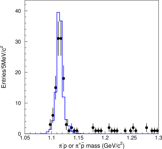
Figure 2: Mass distribution of $\pi^{+}\overline{p}$ ($\pi^{-}p$) recoiling against a $\Lambda$ ($\overline{\Lambda}$) (mass $<1.15$ GeV) for events in the $\chi_{cJ}$ mass region. Dots with error bars are data and the histogram is the Monte Carlo simulation, normalized to the $\Lambda$ signal region (two entries per event).

After requiring that both the $\pi^{+}\overline{p}$ and the $\pi^{-}p$ mass lie within twice the mass resolution around the nominal $\Lambda$ mass, the $\Lambda\overline{\Lambda}$ invariant mass distribution shown in Fig. 3 is obtained. There are clear $\chi_{c0}$, $\chi_{c1}$, and $\chi_{c2}\rightarrow\Lambda\overline{\Lambda}$ signals with low background, estimated using $\Lambda$ mass side band events. The highest peak around the $\psi(2S)$ mass is due to $\psi(2S)\rightarrow\Lambda\overline{\Lambda}$ with a fake photon.

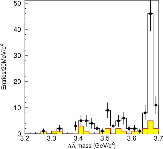
Figure 3: Mass distribution of $\Lambda\overline{\Lambda}$ candidates. Histogram with error bars is data, and the shaded histogram is from $\Lambda$ side bands events (normalized).

Fig. 4 shows the energy deposited in the BSC of the proton track versus the antiproton track for events selected as $\chi_{cJ}\rightarrow\Lambda\overline{\Lambda}$. Since the antiproton will frequently annihilate in the detector, much of the energy of the annihilation products may be detected in the BSC. The scatterplot is consistent with these expectations, indicating the two tracks are really the proton and anti-proton.

Figure 4: Energy deposited in the BSC of the proton and antiproton tracks for selected $\chi_{cJ}\rightarrow\Lambda\overline{\Lambda}$ events.

Fig. 5 shows the distribution of secondary vertices in the $xy$ plane of $\gamma\Lambda\overline{\Lambda}$ candidates in the $\chi_{cJ}$ mass region (error bars). This distribution shows good agreement with the secondary vertex distribution of selected $\psi(2S)\rightarrow\Lambda\overline{\Lambda}$ events (histogram), but is significantly different from the vertex distribution of $\psi(2S)\rightarrow\pi^{+}\pi^{-}J/\psi$, $J/\psi\rightarrow p\overline{p}$ events (stars), where no secondary vertex is expected. This indicates the events in the $\chi_{cJ}$ mass region are real $\Lambda\overline{\Lambda}$.

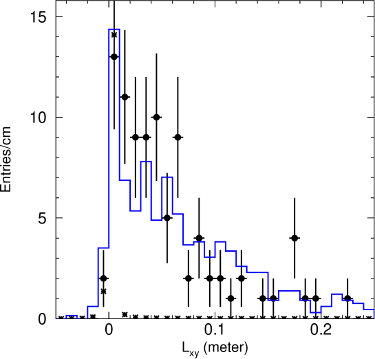
Figure 5: Secondary vertex distributions. Dots with error bars are for events with their mass in the $\chi_{cJ}$ mass region, the histogram is for selected $\psi(2S)\rightarrow\Lambda\overline{\Lambda}$ events, and the asterisks are for selected $\psi(2S)\rightarrow\pi^{+}\pi^{-}J/\psi$, $J/\psi\rightarrow p\overline{p}$ events. The dots and histogram are normalized for greater than 1 cm, and the normalization for the asterisks is arbitrary.

III.1 Remaining backgrounds

Background from non $\Lambda\overline{\Lambda}$ events is estimated from the $\Lambda$ mass sidebands as shown in Fig. 3, and this can be described in fitting the $\Lambda\overline{\Lambda}$ mass spectrum by a linear background. The background from channels with $\Lambda\overline{\Lambda}$ production, including $\psi(2S)\rightarrow\Lambda\overline{\Lambda}$, $\psi(2S)\rightarrow\Sigma^{0}\overline{\Sigma^{0}}$, $\psi(2S)\rightarrow\Lambda\overline{\Sigma^{0}}+c.c.$, $\psi(2S)\rightarrow\Xi^{0}\overline{\Sigma^{0}}+c.c.$, $\psi(2S)\rightarrow\gamma\chi_{cJ},\chi_{cJ}\rightarrow\Sigma^{0}\overline{\Sigma^{0}}\rightarrow\gamma\gamma\Lambda\overline{\Lambda}$, and $\psi(2S)\rightarrow\pi^{+}\pi^{-}J/\psi\rightarrow\pi^{+}\pi^{-}p\overline{p}$, are simulated by Monte Carlo. By using the branching ratios of $\psi(2S)\rightarrow\Lambda\overline{\Lambda}$, $\psi(2S)\rightarrow\Sigma^{0}\overline{\Sigma^{0}}$, and $\psi(2S)\rightarrow\pi^{+}\pi^{-}J/\psi\rightarrow\pi^{+}\pi^{-}p\overline{p}$ measured by previous experiments pdg , and naively assuming $\psi(2S)\rightarrow\Lambda\overline{\Sigma^{0}}+c.c.$ and $\psi(2S)\rightarrow\Xi^{0}\overline{\Sigma^{0}}+c.c.$ are one order of magnitude smaller than $\psi(2S)\rightarrow\Lambda\overline{\Lambda}$ and $\psi(2S)\rightarrow\Sigma^{0}\overline{\Sigma^{0}}$, and $\chi_{cJ}\rightarrow\Sigma^{0}\overline{\Sigma^{0}}$ is about the same as $\chi_{cJ}\rightarrow\Lambda\overline{\Lambda}$, we obtain the expected total background plotted in Fig. 6. The curve in this plot indicates the best fit of the background mass spectrum from 3.2 to 3.65 GeV/$c^{2}$. The background from events with more photons is smaller, and Monte Carlo simulation of $\psi(2S)\rightarrow\Xi^{0}\overline{\Xi^{0}}$ indicates that its contamination to the $\chi_{c}$ signal is negligible.

Figure 6: Invariant mass distribution of $\Lambda\overline{\Lambda}$ selected from Monte Carlo simulated background events normalized to the total number of $\psi(2S)$ events in the data sample. The curve shows the best fit of the mass spectrum below 3.65 GeV/$c^{2}$.

III.2 Fit to the mass spectrum

Fixing the mass resolutions at their Monte Carlo predicted values ($(12.7\pm 0.9)~{}\hbox{MeV}/c^{2}$, $(9.4\pm 0.3)~{}\hbox{MeV}/c^{2}$ and $(9.8\pm 0.4)~{}\hbox{MeV}/c^{2}$ for $\chi_{c0}$, $\chi_{c1}$ and $\chi_{c2}$, respectively), and fixing the widths of the three $\chi_{cJ}$ states to their world average values pdg , the mass spectrum was fit with three Breit-Wigner functions folded with Gaussian resolutions and background, including a linear term representing the non $\Lambda\overline{\Lambda}$ background and a component described in the previous subsection representing the $\Lambda\overline{\Lambda}$ background with the global normalization factor floating to take into account possible systematic bias in the background estimation (mainly branching ratio uncertainties). The unbinned maximum likelihood method was used to fit the events with $\Lambda\overline{\Lambda}$ mass between 3.22 and 3.64 $\hbox{GeV}/c^{2}$, and a likelihood probability of 27% was obtained, indicating a reliable fit. The number of events with errors determined from the fit are $15.2^{+4.2}_{-4.0}$, $9.0^{+3.5}_{-3.1}$, and $8.3^{+3.7}_{-3.4}$ for $\chi_{c0}$, $\chi_{c1}$ and $\chi_{c2}$, respectively. The statistical significances of the three states are $4.5\sigma$, $3.5\sigma$ and $2.6\sigma$. Fig. 7 shows the fit result, and the fitted masses are $(3425.6\pm 6.3)\hbox{MeV}/c^{2}$, $(3508.5\pm 3.9)~{}\hbox{MeV}/c^{2}$ and $(3560.3\pm 4.6)~{}\hbox{MeV}/c^{2}$ for $\chi_{c0}$, $\chi_{c1}$ and $\chi_{c2}$, respectively, in agreement with the world average values pdg . The detection efficiencies from the Monte Carlo simulation were determined to be $\varepsilon_{\chi_{c0}}^{MC}=(6.07\pm 0.24)\%$, $\varepsilon_{\chi_{c1}}^{MC}=(6.65\pm 0.25)\%$ and $\varepsilon_{\chi_{c2}}^{MC}=(6.09\pm 0.24)\%$, where the errors come from the limited statistics of the Monte Carlo samples.

Figure 7: Mass distribution of $\gamma\Lambda\overline{\Lambda}$ candidates fitted with three resolution smeared Breit-Wigner functions and background, as described in the text.

IV Number of $\psi(2S)$ events

The number of $\psi(2S)$ events is determined using $\psi(2S)\rightarrow\pi^{+}\pi^{-}J/\psi,J/\psi\rightarrow p\overline{p}$. There are many advantages in using this channel to determine the number of events:

1. It has the same kind of charged tracks as the channel of interest, and the momenta in these two channels are similar, so that in the branching ratio measurement, the systematic bias in tracking, kinematic fit, triggering, particle ID, geometric acceptance of charged tracks, etc. will cancel out.

2. It is easy to select, and the error on the branching ratio is small ($(2.12\pm 0.10)\times 10^{-3}$ for the world average) pdg .

The selection criteria of this channel are the same as for the $\chi_{cJ}\rightarrow\Lambda\overline{\Lambda}$ analysis, except the photon is not considered. The invariant masses of $\pi^{-}p$ and $\pi^{+}\overline{p}$ are required to not be in the $\Lambda$ mass region to remove $\psi(2S)\rightarrow\Lambda\overline{\Lambda}$ background. Fig. 8 shows the $p\overline{p}$ invariant mass distributions of both data and Monte Carlo. There is a huge $J/\psi$ signal on top of very low background.

Figure 8: Distribution of $p\overline{p}$ invariant mass of $\psi(2S)\rightarrow\pi^{+}\pi^{-}J/\psi,J/\psi\rightarrow p\overline{p}$ data (top) and Monte Carlo (bottom).

The number of $J/\psi\rightarrow p\overline{p}$ events is estimated by subtracting sideband events for $p\overline{p}$ invariant mass regions from 3.0 to 3.05 GeV/c² and from 3.15 to 3.2 GeV/c² from the signal region ($p\overline{p}$ invariant mass from 3.05 to 3.15 GeV/c²), giving

$$n^{obs}_{J/\psi\rightarrow p\overline{p}}=1826\pm 44.$$

Using the same method, the efficiency is determined using Monte Carlo data as

$$\varepsilon=(17.88\pm 0.12)\%.$$

Using the BES branching ratio for $\psi(2S)\rightarrow\pi^{+}\pi^{-}J/\psi$ (($32.3\pm 1.4)\%$ bespsp ) and the PDG branching ratio for $J/\psi\rightarrow p\overline{p}$ ($(2.12\pm 0.10)\times 10^{-3}$ pdg ), the number of $\psi(2S)$ events is obtained

$$N_{\psi(2S)} = \frac{n^{obs}_{J/\psi\rightarrow p\overline{p}}/\varepsilon}{{\cal B}(\psi(2S)\rightarrow\pi^{+}\pi^{-}J/\psi){\cal B}(J/\psi\rightarrow p\overline{p})}$$

$$= (14.91\pm 0.36\pm 1.13)\times 10^{6},$$

where the first error is statistical and the second is systematic, including the statistical error of the efficiency, the errors from the two branching ratios used, and the uncertainty due to the Monte Carlo simulation of the angular distributions.

It should be noted that the efficiency correction factors due to the differences between data and Monte Carlo data in the particle ID, the kinematic fit, tracking, etc. are not considered, because the same differences exist in the $\chi_{cJ}\rightarrow\Lambda\overline{\Lambda}$ analysis and will cancel in the $\chi_{cJ}\rightarrow\Lambda\overline{\Lambda}$ branching ratio measurement.

As a consistency check, one can apply the particle ID correction factor ($1.043\pm 0.011$) and kinematic fitting correction factor ($0.943\pm 0.010$), which are measured in following sections. One then obtains $N_{\psi(2S)}=(15.16\pm 0.37\pm 1.16)\times 10^{6}$, which agrees with the number of $\psi(2S)$ events determined using either inclusive $\psi(2S)\rightarrow\pi^{+}\pi^{-}J/\psi$ or inclusive hadrons.

V Efficiency correction and systematic errors

The systematic errors in the branching ratio measurements come from the efficiencies of the photon ID, particle ID, kinematic fitting, low energy photon detection, MDC tracking, the branching ratios used, the number of $\psi(2S)$ events, the $\Lambda$ mass cut, etc.

V.1 Photon ID

The fake photon multiplicity distributions in both data and Monte Carlo simulation are checked with $\psi(2S)\rightarrow\pi^{+}\pi^{-}J/\psi,J/\psi\rightarrow p\overline{p}$ events. The Monte Carlo predicts too many fake photons at very low energy (less than 50 MeV). Using a photon energy cut at 50 MeV or reweighting the Monte Carlo events with the measured fake photon multiplicity distribution indicates that the Monte Carlo simulates the data with a precision of 4%. This will be taken as the systematic error on the photon ID.

V.2 Particle ID

Samples of $\pi^{+}$, $\pi^{-}$, $p$, and $\overline{p}$ tracks are selected in $\psi(2S)\rightarrow\pi^{+}\pi^{-}J/\psi,J/\psi\rightarrow p\overline{p}$ events by requiring a good kinematic fit to this process and good particle identification of the other three charged tracks involved. This allows a measurement of the particle ID efficiency, and a correction factor of $1.043\pm 0.011$ to the Monte Carlo efficiency is found for the channels that we are studying. The error is from the limited statistics of the samples used and is taken as the systematic error of the particle ID.

V.3 Kinematic fit

The bias due to the kinematic fitting is caused by differences between data and Monte Carlo data in the fitted momentum and error matrix of the charged track and differences in the measurement of the energy and the direction of the neutral track and their uncertainties. The effect is studied for charged tracks and neutral tracks separately.

V.3.1 Charged tracks

The bias from the kinematic fit of the charged tracks was checked using $\psi(2S)\rightarrow\pi^{+}\pi^{-}J/\psi$, $J/\psi\rightarrow p\overline{p}$ events. This channel is very clean and can be selected without the help of a kinematic fit. By comparing the number of events with and without a kinematic fit, the efficiencies for $prob_{\chi^{2}}>1\%$ are measured to be $(85.14\pm 0.92)\%$ and $(90.32\pm 0.24)\%$ for data and Monte Carlo, respectively. This results in a correction factor for the Monte Carlo efficiency of $0.943\pm 0.010$ for this specific channel.

V.3.2 Neutral tracks

The effect of neutral track measurement is studied using $\psi(2S)\rightarrow\gamma\chi_{cJ},\chi_{cJ}\rightarrow\pi^{+}\pi^{-}p\overline{p}$ events. A careful calibration of the neutral cluster information in the BSC (including the energy and direction measurement and their errors) was performed using radiative Bhabha events from the same $\psi(2S)$ data set. By applying this calibration to both data and Monte Carlo, the relative changes in the branching ratios of $\chi_{cJ}\rightarrow\pi^{+}\pi^{-}p\overline{p}$ are measured to be 1.1%, 1.9% and 4.2% for $\chi_{c0}$, $\chi_{c1}$ and $\chi_{c2}$, respectively. No corrections to the efficiencies are made; the largest difference (4.2%) is taken as the systematic error in the measurement of neutral tracks.

V.4 Photon detection efficiency

The low energy photon detection efficiency is studied with $\psi(2S)\rightarrow\pi^{+}\pi^{-}J/\psi$, $J/\psi\rightarrow\pi^{+}\pi^{-}\pi^{0}$ events produced in the same data sample used for the $\chi_{cJ}$ analysis. We assume the lower momentum positive and negative charged tracks are the $\pi^{+}$ and $\pi^{-}$ from $\psi(2S)$ decays, and the largest energy neutral cluster is a photon from the $\pi^{0}$ decay. Assuming the second photon from the $\pi^{0}$ decays is missing, we do a two constraint kinematic fit requiring all the final particles come from $\psi(2S)$ decays and the two photons form a $\pi^{0}$. The fitted four-momentum of the second photon is taken as a test beam into the detector and used to determine the detection efficiency. A total of 2901 photons are selected for the efficiency study. The same analysis is performed with Monte Carlo events, and agreement between data and Monte Carlo data is observed at a precision of $8\%$ for the photons accompanying $\chi_{c0}$, $\chi_{c1}$ and $\chi_{c2}$.

For converted photons, no specific study was performed since this occurs for only a very small fraction of the events (less than 1%), and the difference between data and Monte Carlo simulation should be even smaller and negligible compared to the quoted systematic error for the photon efficiencies.

V.5 Other systematic errors

The angular distributions of the photon accompanying the $\chi_{cJ}$s and the angular distributions of the $\Lambda$ or $\overline{\Lambda}$ decays may cause a systematic error at the 10% level. This is determined by comparing different theoretical models for the angular distributions. The uncertainty in the angular distribution of the proton in $J/\psi$ decays results in a 4% error in the determination of the number of $\psi(2S)$ events.

The Monte Carlo simulated mass resolution may have a bias at the 10% level. This is determined from the comparison of $\Lambda$ and $J/\psi$ signals in various channels involved in this analysis. Changing the mass resolutions used in fitting the $\chi_{cJ}$ mass plot produces small changes in the number of events; the maximum change in the three cases is around 3%. This is taken as the systematic error due to the mass resolution uncertainty.

The background estimation, including the uncertainties in the branching ratios used, the uncertainties in the simulation of the contamination probability, the parameterization of the background shape, and the fitting range used, etc., causes an uncertainty at the 10% level. The systematic errors on the branching ratios used, like ${\cal B}(\psi(2S)\rightarrow\pi^{+}\pi^{-}J/\psi)$, ${\cal B}(J/\psi\rightarrow p\overline{p})$, ${\cal B}(\psi(2S)\rightarrow\gamma\chi_{cJ})$ and ${\cal B}(\Lambda\rightarrow\pi^{-}p)$ are obtained from other experiments bespsp ; pdg .

V.6 Total systematic error

Table. 1 lists the systematic errors from all sources, as well as the correction factors to the Monte Carlo efficiency for particle ID and the kinematic fitting of charged tracks. Since these two correction factors cancel out in the calculation of branching ratios, there are no corrections to the efficiencies determined by Monte Carlo simulation for the $\chi_{c0}$, $\chi_{c1}$ and $\chi_{c2}$ branching ratios, and their errors are not considered in the summation.

Table 1: Summary of systematic errors and the efficiency correction factors. Efficiency correction factors are only determined for the particle ID and the kinematic fitting of charged tracks. Since these correction factors cancel in the branching ratio calculation, they are not used.

Source	$\chi_{c0}$	$\chi_{c1}$	$\chi_{c2}$
MC statistics	4.0%	3.8%	4.0%
Fake photon	4%
Particle ID	1.043$\pm$0.011
4C-fit (chrg)	0.943$\pm$0.010
4C-fit (neut)	4.2%
Phot. eff.	8%
Gamma conversion	$<$1%
Angular distr.	10%
Mass resolution	3%
Background	10%
$\psi(2S)$ number	8.0%
${\cal B}(\Lambda\rightarrow\pi^{-}p)$	1.6%
${\cal B}(\psi(2S)\rightarrow\gamma\chi_{cJ})$	9.2%	8.3%	8.8%
Total systematic error	22%	21%	22%

VI Results and discussions

The branching ratios of $\chi_{cJ}\rightarrow\Lambda\overline{\Lambda}$ can be calculated with

$${\cal B}(\chi_{cJ}\rightarrow\Lambda\overline{\Lambda})=\left.\frac{n^{obs}/\varepsilon}{N_{\psi(2S)}{\cal B}(\psi(2S)\rightarrow\gamma\chi_{cJ}){\cal B}(\Lambda\rightarrow\pi^{-}p)^{2}}\right.~{}.$$

Using numbers from above, one gets

$${\cal B}(\chi_{c0}\rightarrow\Lambda\overline{\Lambda})=(4.7^{+1.3}_{-1.2}\pm 1.0)\times 10^{-4},$$

$${\cal B}(\chi_{c1}\rightarrow\Lambda\overline{\Lambda})=(2.6^{+1.0}_{-0.9}\pm 0.6)\times 10^{-4},$$

$${\cal B}(\chi_{c2}\rightarrow\Lambda\overline{\Lambda})=(3.3^{+1.5}_{-1.3}\pm 0.7)\times 10^{-4},$$

where the first errors are statistical and the second are systematic. The numbers used and results are summarized in Table. 2.

Table 2: Summary of numbers used in the branching ratio calculation and branching ratio results. $R_{{\cal B}}$, defined in the text, is the relative branching ratio of $\chi_{c0}\rightarrow\Lambda\overline{\Lambda}$ to that of $\psi(2S)\rightarrow\pi^{+}\pi^{-}J/\psi$.

quantity	$\chi_{c0}$	$\chi_{c1}$	$\chi_{c2}$
$n^{obs}$	$15.2^{+4.2}_{-4.0}$	$9.0^{+3.5}_{-3.1}$	$8.3^{+3.7}_{-3.4}$
$\varepsilon$ (%)	$6.07\pm 0.24$	$6.65\pm 0.25$	$6.09\pm 0.24$
$N_{\psi(2S)}(10^{6})$	$14.9\pm 1.2$
${\cal B}(\Lambda\rightarrow\pi^{-}p)$ pdg	$0.639\pm 0.005$
${\cal B}(\psi(2S)\rightarrow\gamma\chi_{cJ})$ (%) pdg	$8.7\pm 0.8$	$8.4\pm 0.7$	$6.8\pm 0.6$
${\cal B}(\chi_{cJ}\rightarrow\Lambda\overline{\Lambda})(10^{-4})$	$4.7^{+1.3}_{-1.2}\pm 1.0$	$2.6^{+1.0}_{-0.9}\pm 0.6$	$3.3^{+1.5}_{-1.3}\pm 0.7$
$n^{obs}_{\pi^{+}\pi^{-}J/\psi}$	$1826\pm 44$
$\varepsilon_{\pi^{+}\pi^{-}J/\psi}$ (%)	$17.88\pm 0.12$
$R_{{\cal B}}(10^{-2})$	$2.45^{+0.68}_{-0.65}\pm 0.46$	$1.33^{+0.52}_{-0.46}\pm 0.25$	$1.33^{+0.59}_{-0.55}\pm 0.25$

Compared with the corresponding branching ratios of $\chi_{cJ}\rightarrow p\overline{p}$ pdg , the branching ratios of $\chi_{c1}$ and $\chi_{c2}\rightarrow\Lambda\overline{\Lambda}$ agree with the corresponding branching ratios to $p\overline{p}$ within two sigma. This is somewhat in contradiction with the expectations from Ref. wong , although the errors are large.

As for $\chi_{c0}\rightarrow\Lambda\overline{\Lambda}$, the measured value agrees with the $p\overline{p}$ measurements from BES and E835 width ; e835 within 2 standard deviations. One should also note that there is no prediction for ${\cal B}(\chi_{c0}\rightarrow\Lambda\overline{\Lambda})$.

What we actually measure in this analysis is the relative branching ratio of $\chi_{c0}\rightarrow\Lambda\overline{\Lambda}$ to $\psi(2S)\rightarrow\pi^{+}\pi^{-}J/\psi$. The relative branching ratio is found with the following formula

$$R_{{\cal B}} = \frac{{\cal B}(\psi(2S)\rightarrow\gamma\chi_{cJ})\cdot{\cal B}(\chi_{cJ}\rightarrow\Lambda\overline{\Lambda})\cdot{\cal B}(\Lambda\rightarrow\pi^{-}p)^{2}}{{\cal B}(\psi(2S)\rightarrow\pi^{+}\pi^{-}J/\psi)\cdot{\cal B}(J/\psi\rightarrow p\overline{p})}$$

$$= \frac{n^{obs}/\varepsilon}{n^{obs}_{\pi^{+}\pi^{-}J/\psi}/\varepsilon_{\pi^{+}\pi^{-}J/\psi}}.$$

These results are also shown in Table 2.

VII Summary

$\Lambda\overline{\Lambda}$ events are observed for the first time in $\chi_{cJ}$ decays using the BESII 15 million $\psi(2S)$ event sample, and corresponding branching ratios are determined. The results on $\chi_{c1}$ and $\chi_{c2}$ decays only agree marginally with model predictions.

References

(1) See, for example G.T. Bodwin,
E. Braaten and G.P. Lepage,
Phys. Rev. D51, 1125 (1995);
Han-Wen Huang and Kuang-Ta Chao,
Phys. Rev. D54, 6850 (1996);
J. Bolz, P. Kroll and G. A. Schuler,
Phys. Lett. B392, 198 (1997).
(2) J. Z. Bai et al. (BES Collab.),
Phys. Rev. Lett. 81, 3091 (1998).
(3) S. M. Wong, Eur. Phys. J. C14, 643 (2000).
(4) K. Hagiwara et al. (Particle Data Group),
Phys. Rev. D66, 010001 (2002).
(5) J. Z. Bai et al. (BES Collab.), Nucl. Instr. Meth.
A344, 319 (1994).
(6) J. Z. Bai et al. (BES Collab.), Nucl. Instr. Meth.
A458, 627 (2001).
(7) J. Z. Bai et al. (BES Collab.),
Phys. Rev. D58, 092006 (1998).
(8) J. Z. Bai et al. (BES Collab.),
Phys. Rev. D60, 072001 (1999).
(9) J. Z. Bai et al. (BES Collab.),
Phys. Lett. B550, 24 (2002).
(10) S. Bagnasco et al. (E835 Collab.),
Phys. Lett. B533, 237 (2002);
M. Ambrogiani et al. (E835 Collab.),
Phys. Rev. Lett. 83, 2902 (1999).