High statistics measurement of $K_{e4}$ decay properties

Abstract

We report experimental details and results of a new measurement of the decay $K^{+}\rightarrow\pi^{+}\pi^{-}e^{+}\nu_{e}$ ($K_{e4}$). A sample of more than 400,000 $K_{e4}$ events with low background has been collected by Experiment 865 at the Brookhaven Alternate Gradient Synchrotron. From these data, the branching ratio $(4.11\pm 0.01\pm 0.11)\cdot 10^{-5}$ and the $\pi\pi$ invariant mass dependence of the form factors $F$, $G$, and $H$ of the weak hadronic current as well as the phase shift difference $\delta^{0}_{0}-\delta^{1}_{1}$ for $\pi\pi$-scattering were extracted. Using constraints based on analyticity and chiral symmetry, a new value with considerably improved accuracy for the $s$-wave $\pi\pi$-scattering length $a^{0}_{0}$ has been obtained also: $a_{0}^{0}=0.216\pm 0.013\,({\rm stat.})\pm 0.002\,({\rm syst.})\pm 0.002\,({\rm theor.})$.

I Introduction

Among the long list of possible charged kaon decays the rare $K_{e4}$ decay branch $(K^{\pm}\rightarrow\pi^{+}\pi^{-}e^{\pm}\nu_{e}(\bar{\nu}_{e}))$ has received particular attention, because it was recognized shabalin63 , almost coincident with the observation of the first event for this decay 40 years ago koller62 , that it could provide important information on the structure of the weak hadronic currents and also on $\pi\pi$ scattering at low energies. The final state interaction of the two pions was expected to manifest itself in an angular correlation between the decay products, namely an asymmetry of the lepton distribution with respect to the plane formed by the two pion momenta. This asymmetry is directly related to the difference between the $s$- and $p$-wave scattering phase. What made this four-body semileptonic decay attractive despite its low branching ratio, which was then predicted to be of order $10^{-5}$ okun60 , is that the two pions are the only hadrons in the final state. For all other reactions used to study the $\pi\pi$ interaction, e.g. $\pi^{-}p\rightarrow\pi^{-}\pi^{+}n$, there is at least one other hadron present in the final state. Thus experimental studies of the $K_{e4}$-decay were seen as the cleanest method to determine the isospin zero, angular momentum zero scattering length $a_{0}^{0}$. Since early experiments birge65 ; ely69 ; schweinberger71 ; bourquin71 ; beier72 observed only a few hundred events each, it was not until 1977, when the Geneva-Saclay experiment rosselet77 gathered about 30,000 events, that a measurement was made of this quantity to 20% accuracy.

Since then no new data became available until Experiment 865 at the Brookhaven Alternating Gradient Synchrotron collected 400,000 $K_{e4}$ events. We report here the details of the analysis of these data, some of which have been communicated earlier pislak01 . A promising alternative way to study $\pi\pi$-interactions through a measurement of the lifetime of the $\pi\pi$-atom is followed in the DIRAC experiment at CERN dirac , which has not yet yielded a definitive result.

The theoretical analysis of $\pi\pi$-interactions at low energies is intimately linked to the development of chiral quantum chromodynamics perturbation theory (ChPT) ChPT ; leutwyler01 ; honnef02 . In this approach, the fact that standard QCD perturbation theory is not directly applicable at low energies because the strong coupling becomes large, is circumvented through a systematic expansion of the observables in terms of external momenta and of light quark masses. The spontaneous breakdown of the underlying chiral symmetry is associated with the quark-antiquark vacuum expectation value, the so-called quark condensate $\langle 0|\overline{q}q|0\rangle$. It is normally assumed to be of natural size, or equivalently that the Gell-Mann–Oakes–Renner formula gellmann68 for the pion mass

$$m_{\pi}^{2}\simeq\frac{1}{F_{\pi}^{2}}(m_{u}+m_{d})\langle 0|\overline{q}q|0\rangle$$ (1)

has only small corrections. Here $F_{\pi}\simeq 93$ MeV is the pion decay constant. This assumption does not have to be made, as the authors of a less restrictive version of chiral perturbation theory (GChPT) GChPT ; knecht95 pointed out. The measurement of the $\pi\pi$ threshold parameters has been advocated as one of the areas where a significant difference between the two approaches could be observed. ChPT, however, makes firm predictions for the scattering length. The tree level calculation ($\mathcal{O}(p^{2})$ weinberg66 ) yields $a_{0}^{0}=0.156$ (in this paper we use units of $m_{\pi}^{-1}$ for the scattering length). The one-loop ($\mathcal{O}(p^{4})$, $a_{0}^{0}=0.201\pm 0.01$ gasser83 ) and the two loop calculation (($\mathcal{O}(p^{6})$, $a_{0}^{0}=0.217$ bijnens96 ) show satisfactory convergence. The most recent calculation colangelo00 ; colangelo01b matches the known chiral perturbation theory representation of the $\pi\pi$ scattering amplitude to two loops bijnens96 with the dispersive representation that follows from the Roy equations roy71 ; ananthanarayan00 , resulting in the prediction $a_{0}^{0}=0.220\pm 0.005$. The high precision of this prediction has to be contrasted with the experimental value $a_{0}^{0}=(0.26\pm 0.05)$ extracted from the Geneva-Saclay experiment rosselet77 using the Roy equations and some peripheral $\pi N\rightarrow\pi\pi N$ data nagels79 .

The form factors appearing in the weak hadronic current in the $K_{e4}$ decay matrix element, have also been extensively used for the determination of the parameters of the ChPT Hamiltonian talavera00 ; talavera01 . This program would clearly benefit from lower experimental uncertainties.

II Theoretical background for the analysis of $K_{e4}$ decay

II.1 Kinematics

The decay

$$K^{+}(p)\rightarrow\pi^{+}(p_{1})\pi^{-}(p_{2})e^{+}(p_{e})\nu_{e}(p_{\nu})$$ (2)

can most conveniently be treated ke494 by using three reference frames, as illustrated in Fig. 1: (1) the $K^{+}$ rest system ($\Sigma_{K}$), (2) the $\pi^{+}\pi^{-}$ rest system ($\Sigma_{\pi\pi}$) and (3) the $e^{+}\nu_{e}$ rest system ($\Sigma_{e\nu}$).

Figure 1: Kinematic quantities used in the analysis of $K_{e4}$ decay.

The kinematics of the $K_{e4}$ decay are then fully described by five variables, introduced by Cabibbo and Maksymowicz cabibbo65 :

1. $s_{\pi}=M_{\pi\pi}^{2}$, the invariant mass squared of the dipion;

2. $s_{e}=M_{e\nu}^{2}$, the invariant mass squared of the dilepton;

3. $\theta_{\pi}$, the angle of the $\pi^{+}$ in $\Sigma_{\pi\pi}$ with respect to the direction of flight of the dipion in $\Sigma_{K}$;

4. $\theta_{e}$, the angle of the $e^{+}$ in $\Sigma_{e\nu}$ with respect to the direction of flight of the dilepton in $\Sigma_{K}$;

5. $\phi$, the angle between the plane formed by the two pions and the corresponding plane formed by the two leptons.

It is useful for the following discussion to introduce the combinations $P$, $Q$ and $L$ of the momentum four vectors $p_{1}$, $p_{2}$, $p_{e}$ and $p_{\nu}$ defined in Eq. (2) and two scalar products derived from them

$$P=p_{1}+p_{2}\;,\;\;Q=p_{1}-p_{2}\;,\;\;L=p_{e}+p_{\nu}\;,$$ (3)

$$Q^{2}=4m_{\pi}^{2}-s_{\pi}\;,\;\;P\cdot L=\frac{1}{2}(m_{K}^{2}-s_{\pi}-s_{e})\;,$$ (4)

$$X=[(P\cdot L)^{2}-s_{\pi}s_{e}]^{1/2}\;,\;\;\sigma_{\pi}=(1-4m_{\pi}^{2}/s_{\pi})^{1/2}\;.$$ (5)

II.2 Matrix element

The matrix element is written as

$$M=\frac{G_{F}}{\sqrt{2}}V^{*}_{us}\overline{u}(p_{\nu})\gamma_{\mu}(1-\gamma_{5})v(p_{e})(V^{\mu}-A^{\mu})\;.$$ (6)

The vector current $V^{\mu}$ and the axial vector current $A^{\mu}$ have to be Lorentz invariant four-vectors:

$$A^{\mu} = \frac{1}{m_{K}}\left(FP^{\mu}+GQ^{\mu}+RL^{\mu}\right)\;,$$

$$V^{\mu} = \frac{H}{m_{K}^{3}}\epsilon^{\mu\nu\rho\sigma}L_{\nu}P_{\rho}Q_{\sigma}\;.$$ (7)

The kaon mass $m_{K}$ was inserted to make the form factors $F$, $G$, $R$ and $H$ dimensionless complex functions of $p_{1}\cdot p_{2}$, $p_{1}\cdot p$ and $p_{2}\cdot p$ or equivalent of $s_{\pi}$, $s_{e}$ and $\theta_{\pi}$.

II.3 Decay rate

The decay rate following from the matrix element given in Eq. 6 and neglecting terms proportional to $m_{2}^{e}/s_{e}$ is given by pais67

$$d\Gamma_{5} = \frac{G_{F}^{2}V^{2}_{us}}{2^{12}\pi^{6}m_{K}^{5}}X\sigma_{\pi}J_{5}(s_{\pi},s_{e},\theta_{\pi},\theta_{e},\phi)ds_{\pi}ds_{e}d(\cos\theta_{\pi})d(\cos\theta_{e})d\phi\;,$$ (8)

$$J_{5} = I_{1}+I_{2}\cos{2\theta_{e}}+I_{3}\sin^{2}{\theta_{e}}\cos{2\phi}+I_{4}\sin{2\theta_{e}}\cos{\phi}+I_{5}\sin{\theta_{e}}\cos{\phi}$$ (9)

$$+I_{6}\cos{\theta_{e}}+I_{7}\sin{\theta_{e}}\sin{\phi}+I_{8}\sin{2\theta_{e}}\sin{\phi}+I_{9}\sin^{2}{\theta_{e}}\sin^{2}{\phi}\;,$$

Again neglecting terms proportional to $m_{e}^{2}/s_{e}$ the functions $I_{i}$ are given by

$$I_{1} = \frac{1}{8}\left\{2|F_{1}|^{2}+3\left(|F_{2}|^{2}+|F_{3}|^{2}\right)\sin^{2}\theta_{\pi}\right\}\;,\hskip 8.53581ptI_{2}=-\frac{1}{8}\left\{2|F_{1}|^{2}-\left(|F_{2}|^{2}+|F_{3}|^{2}\right)\sin^{2}\theta_{\pi}\right\}\;,$$ (10)

$$I_{3} = -\frac{1}{4}\left\{|F_{2}|^{2}-|F_{3}|^{2}\right\}\sin^{2}\theta_{\pi}\;,\hskip 8.53581ptI_{4}=\frac{1}{2}\mbox{ Re}(F_{1}^{*}F_{2})\sin\theta_{\pi}\;,\hskip 8.53581ptI_{5}=-\mbox{ Re}(F_{1}^{*}F_{3})\sin\theta_{\pi}\;,$$

$$I_{6} = -\mbox{ Re}(F_{2}^{*}F_{3})\sin^{2}\theta_{\pi}\;,\hskip 8.53581ptI_{7}=-\mbox{ Im}(F_{1}^{*}F_{2})\sin\theta_{\pi}\;,\hskip 8.53581ptI_{8}=\frac{1}{2}\mbox{ Im}(F_{1}^{*}F_{3})\sin\theta_{\pi}\;,\hskip 8.53581ptI_{9}=-\frac{1}{2}\mbox{ Im}(F_{2}^{*}F_{3})\sin^{2}\theta_{\pi}\ .$$

The form factors $F$, $G$, and $H$ are contained in the functions $F_{i}$, which are given by

$$F_{1} = XF+\sigma_{\pi}(P\cdot L)\cos\theta_{\pi}\cdot G\;,$$

$$F_{2} = \sigma_{\pi}(s_{\pi}s_{e})^{1/2}G\;,$$

$$F_{3} = \sigma_{\pi}X(s_{\pi}s_{e})^{1/2}\frac{H}{m_{K}^{2}}$$ (11)

The contribution of the form factor $R$ is suppressed by a factor $m_{e}^{2}/s_{e}$ and is therefore negligible. Consequently $R$ cannot be determined from $K_{e4}$ decay.

II.4 Parametrisation of the form factors

As noted above, the form factors $F$, $G$ and $H$ are functions of $\theta_{\pi}$, $s_{\pi}$ and $s_{e}$, and can be determined directly from a fit to the experimental data for sufficiently small bins of these kinematic variables. Alternatively a parametrisation recently introduced by Amorós and Bijnens amoros99 may be used, which is based on a partial wave expansion in the variable $\theta_{\pi}$:

$$F = \left(f_{s}+f_{s}^{\prime}\,q^{2}+f_{s}^{\prime\prime}\,q^{4}+f_{e}(s_{e}/4m_{\pi}^{2})\right)e^{i\delta^{0}_{0}(s_{\pi})}$$

$$+ \tilde{f}_{p}\,(\sigma_{\pi}X/4m_{\pi}^{2})\cos\theta_{\pi}\,e^{i\delta^{1}_{1}(s_{\pi})}$$

$$G = \left(g_{p}+g_{p}^{\prime}\,q^{2}+g_{e}(s_{e}/4m_{\pi}^{2})\right)e^{i\delta^{1}_{1}(s_{\pi})}$$

$$H = \left(h_{p}+h_{p}^{\prime}\,q^{2}\right)e^{i\delta^{1}_{1}(s_{\pi})}\;,$$ (12)

where $q=[(s_{\pi}-4m_{\pi}^{2})/4m_{\pi}^{2}]^{1/2}$ is the pion momentum in $\Sigma_{\pi\pi}$. This parametrisation was constrained by theoretical models and the expected accuracy of the experimental data. It yields 10 new dimensionless form factor parameters $f_{s}$, $f_{s}^{\prime}$, $f_{s}^{\prime\prime}$, $f_{e}$, $\tilde{f}_{p}$, $g_{p}$, $g_{p}^{\prime}$, $g_{e}$, $h_{p}$, and $h_{p}^{\prime}$, which do not depend on any kinematic variables, plus two phase shifts, which can be identified using Watson’s theorem watson52 with the $s$- and $p$-wave (isoscalar and isovector, respectively) $\pi\pi$ scattering phase shifts $\delta_{0}^{0}$ and $\delta_{1}^{1}$, which are still functions of $s_{\pi}$. In our analysis we will additionally assume $f_{e}=\tilde{f}_{e}=g_{e}=h_{p}^{\prime}=0$. The validity of this assumption will be experimentally tested. When Eq. 12 is inserted into Eq. II.3 and then into Eq. 10, it can be observed that the phase shift difference $\delta=\delta_{0}^{0}-\delta_{1}^{1}$ enters via $\cos\delta$ into the terms $I_{1}$, $I_{2}$, $I_{4}$, $I_{5}$, and via $\sin\delta$ into the terms $I_{7}$ and $I_{8}$. Since $\delta<0.3$ with $\cos\delta>0.95$ holds in $K_{e4}$-decay, and the kinematic factors suppress the term $I_{8}$, only the term $I_{7}$ is really relevant, which appears in the decay rate (Eq. 9 and Eq. 8) multiplied by $\sin\phi$. $I_{7}$ and $I_{8}$ are the only odd $\phi$ terms. Hence, as noted by Shabalin shabalin63 , and Pais and Treiman pais67 , the asymmetry of the $\phi$ distribution is the observable that is most sensitive to the phase shifts. This also holds for any other parametrisation of the form factors. The amplitude of the asymmetry is quite small compared to the $\phi$ independent part, as Figures 6 and 9 illustrate. This explains why a very high statistics data sample is needed for an accurate measurement of the phase shift difference.

II.5 $\pi\pi$ Scattering length

To establish a relation between the phase shift $\delta_{0}^{0}$ and the scattering length normally the analytical properties of the $\pi\pi$ scattering amplitudes and crossing relations are used, which lead to dispersion relations contained in the Roy equations roy71 . Ananthanarayan et al. ananthanarayan00 have recently updated earlier treatments morgan94 , which were used in the analysis of $\pi\pi$ scattering data, and solved these equations numerically. Their analysis made use of a phase shift parametrisation originally proposed by Schenk schenk91 :

$$\tan\delta_{\ell}^{I} = \sqrt{1-\frac{4m_{\pi}^{2}}{s_{\pi}}}\;q^{2\ell}\left\{A^{I}_{\ell}+B^{I}_{\ell}q^{2}+C^{I}_{\ell}q^{4}+D^{I}_{\ell}q^{6}\right\}$$ (13)

$$\times \left(\frac{4m_{\pi}^{2}-s^{I}_{\ell}}{s_{\pi}-s^{I}_{\ell}}\right)\,.$$

The solution of the Roy equations implies that the parameters $A^{I}_{\ell}$, $B^{I}_{\ell}$, etc. can be expressed as a function of only two parameters or subtraction constants, which are identified as the $I=0$ and $I=2$ $s$-wave scattering lengths $a_{0}^{0}$ and $a_{0}^{2}$. For example, the first two coefficients of this expression for the $I=\ell=0$ case read as follows coeff

$$A^{0}_{0} = a_{0}^{0}\;,$$

$$B_{0}^{0} = 0.2395+0.9237\Delta a_{0}^{0}-3.352\Delta a_{0}^{2}+0.2817(\Delta a_{0}^{0})^{2}$$

$$+6.335(\Delta a_{0}^{2})^{2}+6.074\Delta a_{0}^{0}\Delta a_{0}^{2}+\ldots\;,$$

$$s_{0}^{0} = 36.83m_{\pi}^{2}\left(1+0.2764\Delta a_{0}^{0}-0.1409\Delta a_{0}^{2}+\ldots\right)$$

$$\simeq (0.847)^{2}\;{\rm GeV}^{2}\;,$$

where $\Delta a_{0}^{0}\equiv a_{0}^{0}-0.220$ and $\Delta a_{0}^{2}\equiv a_{0}^{2}+0.0444$. Although $K_{e4}$ decay allows only $I=0$ and $I=1$ contributions, the use of the crossing relations brings in a modest dependence on the $I=2$ scattering length. The $I=1$ phase shifts at low energies are dominated by the $\rho$ resonance and are furthermore small in the region of interest for $K_{e4}$.

It was recognized by Morgan and Shaw morgan69 that the possible values of $a_{0}^{0}$ and $a_{0}^{2}$ are restricted to a band in the $a_{0}^{0}-a_{0}^{2}$-plane, the so-called universal band. This band is defined as the area which is allowed by $\pi\pi$ scattering data above 0.8 GeV hyams73 ; protopopescu73 and the Roy equations. The allowed range, estimated in the most recent analysis ananthanarayan00 , is shown in Fig. 10. The central curve of this band is given by

$$a_{0}^{2}=-0.0849+0.232\,a_{0}^{0}-0.0865\,(a_{0}^{0})^{2}\;\left[\pm 0.0088\right]\;,$$ (14)

where the figure given in the bracket indicates the width of the band. Figure 2 illustrates the influence of the universal band and how the phase shift difference $\delta=\delta_{0}^{0}-\delta_{1}^{1}$ depends on the scattering length $a_{0}^{0}$.

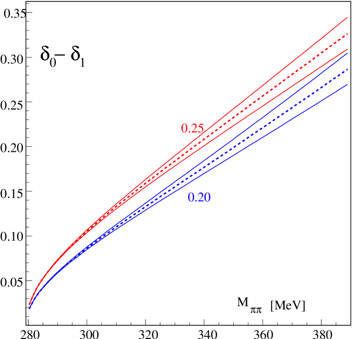
Figure 2: Predictions for the phase shift $\delta$ resulting from Eq. 13 and Eq. 14 for two values of $a_{0}^{0}$. The three curves refer to the upper and lower limit and the center, respectively, of the universal band in the $(a_{0}^{2},a^{0}_{0})$-plane (Eq. 14).

It has recently been shown by Colangelo et al. colangelo01a ; colangelo01b that the width of the allowed band can be considerably reduced to $\left[\pm 0.0008\right]$, if chiral symmetry constraints are imposed in addition. $a_{0}^{2}$ and $a_{0}^{0}$ are then related as

$$\Delta a_{0}^{2}=0.236\Delta a_{0}^{0}-0.61(\Delta a_{0}^{0})^{2}-9.9(\Delta a_{0}^{0})^{3}\;,$$ (15)

where $\Delta a_{0}^{2}$ and $\Delta a_{0}^{0}$ have been defined above. This band is also depicted in Fig. 10 with the label CLG.

In ChPT up to order $\mathcal{O}(p^{4})$ the scattering lengths are linked to two coupling constants $\ell_{3}$ and $\ell_{4}$. For example, $\ell_{3}$ determines the size of the first order correction to the Gell-Mann–Oakes-Renner relation (Eq. 1)  gellmann68 , and is assumed to be a priori unknown in GChPT. Colangelo et al. colangelo01a ; colangelo01b have argued, that both $a_{0}^{0}$ and $a_{0}^{2}$ can be made dependent solely on $\ell_{3}$, if the scalar radius of the pion is used as an additional input to give a relation between $\ell_{3}$ and $\ell_{4}$. This also holds in GChPT, and Eq. 15 results, when $\ell_{4}$ is eliminated. Once the scattering lengths are known experimentally, a constraint for $\ell_{3}$ and consequently for the quark condensate can be derived.

III Experimental set up

III.1 Apparatus

The analysis outlined here is based on data recorded at the Brookhaven Alternate Gradient Synchrotron (AGS) in a dedicated run at reduced beam intensity in 1997, employing the E865 detector. The apparatus, described in great detail in appel02 , is shown in Fig. 3.

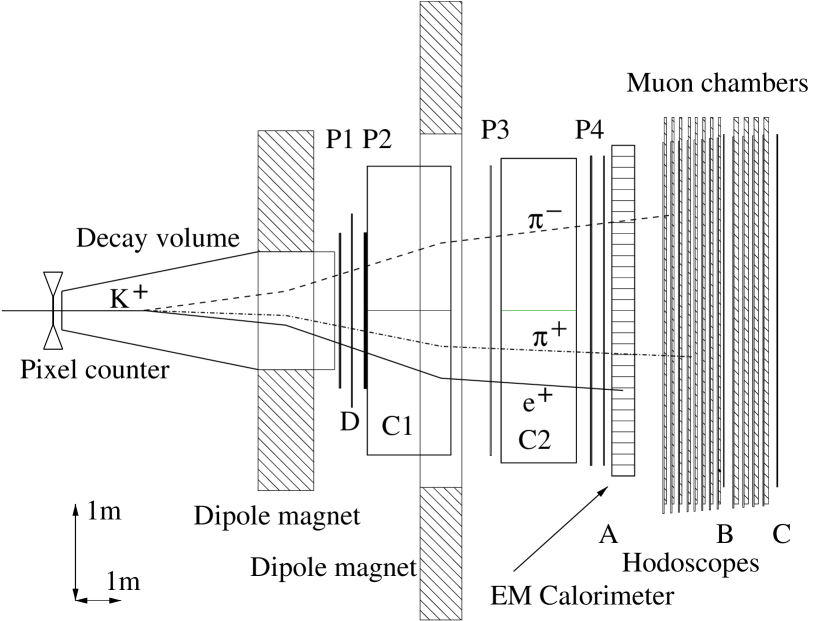
Figure 3: Plan view of the E865 detector. A $K_{e4}$ event is superimposed.

Figure 4: Background contributions: the markers show the data while the solid histogram displays the Monte Carlo simulation. a) Three-pion invariant mass distribution for $K_{e4}$ candidate events, assigning a pion mass to the positron. The small peak at the $K^{+}$ mass arises from $K_{\tau}$ events. b) Total momentum reconstructed from the three charged track momenta. The solid histogram is the sum of the Monte Carlo simulation of $K_{e4}$ events (dashed histogram) and the background from 2-1 accidentals (lower dotted histogram). c) Electron-positron invariant mass $M_{ee}$ assigning electron mass to the reconstructed $\pi^{-}$ for $K_{e4}$ events. $K_{dal}$ events (insert) are characterized by low values of $M_{ee}$.

Here we will mention only its main features. The detector was located in a 6 GeV unseparated beam of approximately $1.5\times 10^{7}$ $K^{+}$ accompanied by about $3\times 10^{8}$ $\pi^{+}$ and protons per machine spill of 1.6-2.8 s duration. About 6% of the kaons accepted by the beam line decayed in the 5 m long evacuated decay volume. The decay products were separated by charge and swept away from the beam by a first dipole magnet. Negatively charged particles were deflected to the left. A second dipole magnet sandwiched between four proportional wire chambers (P1-P4) served as the spectrometer. The wire chambers, each consisting of four wire planes, were deadened in the region where the beam passed. This arrangement yielded a momentum resolution of $\sigma_{P}\simeq 0.003\,P^{2}$ GeV$/c$, where $P$, the momentum of the decay products in GeV$/c$, had a typical range of 0.6 to 3.5. Pions and muons were distinguished from positrons and electrons using two Čerenkov counters, C1 and C2, situated inside and behind the second dipole magnet, and rendered insensitive in the beam region. Both Čerenkov counters, when filled with CH₄ at atmospheric pressure, yielded on average seven photoelectrons, and hence insured an electron identification probability greater than 99 %. An electromagnetic calorimeter of the Shashlyk design atoyan92 , located downstream of P4 further aided the separation of the positrons from other charged decay products. It consisted of 30 modules in the horizontal and 20 modules in the vertical direction, but for the beam region, where $6\times 3$ modules were absent. Module size was 11.4 cm high and 11.4 cm wide perpendicular to the beam direction and 15 radiation length deep. The calorimeter was followed by an array of 12 muon chambers, separated by iron planes, employed to discriminate pions against muons. Four hodoscopes were added to the detector for trigger purposes. The A-hodoscope was situated just upstream of the calorimeter, the B- and C-hodoscopes were embedded in the muon stack, and the D-hodoscope was located between the first two proportional wire chambers. The detector was completed by a pixel counter, installed just upstream of the decay volume, which measured the position of the incoming kaons. This device consisted of an array of 12 (horizontally) by 32 (vertically) scintillating pixels, each with an area of $7\times 7$ mm².

Table 1 summarizes the resolution of the apparatus in the five variables required to describe the kinematics of the $K_{e4}$ decay.

Variable	FWHM
$s_{\pi}$	0.00133	GeV2
$s_{e}$	0.00361	GeV2
$\theta_{\pi}$	0.147	rad
$\theta_{e}$	0.111	rad
$\phi$	0.404	rad

Table 1: Experimental resolutions for the five kinematic variables used in the analysis.

III.2 Trigger requirements

Figure 5: Comparison of the Monte Carlo simulation (histogram) with data (markers with error bars). Left: distance of closest approach $s$ to the common vertex for the three charged tracks; center: missing neutrino mass squared; right: distribution of decay vertices along the beam direction $z$ ($z=0$ at the entrance of the first dipole magnet). The dashed histograms show the background contributions.

The trigger was designed as a multilevel structure with increasing sophistication. The lowest trigger level (T0) indicated the presence of three charged particle tracks, two on the right and one on the left side, each signaled by a coincidence between the A-counter and the corresponding calorimeter module directly behind it (A$\cdot$SH). For each combination of coincidences on the right only a limited, kinematically acceptable region on the left was allowed. To insure that the trigger resulted from particles coming from the decay volume, at least one coincidence on both sides between the D-counter and A$\cdot$SH was required. The next trigger level (T1) demanded the presence of a positron in order to reject events from the $K^{+}\rightarrow\pi^{+}\pi^{+}\pi^{-}$ ($K_{\tau}$) decay, and dismissed all events with evidence for the presence of an electron to eliminate events from $K^{+}\rightarrow\pi^{+}\pi^{0}$ ($\pi^{0}\rightarrow e^{+}e^{-}\gamma$, $K_{\rm dal}$) decay, both rather common decay modes. Consequently, this trigger level required signals in both Čerenkov counters on the right (corresponding to at least 2.5 photoelectrons) and vetoed all events with a signal in either Čerenkov counters on the left (at least 0.25 photoelectrons). The final trigger level (T2) rejected events with a high occupancy in the wire chambers, most likely caused by noise in the read-out electronics. It did not reject many events, but the ones it rejected would have required an exceedingly large amount of computer time in the reconstruction. In addition to $K_{e4}$ candidates, a few prescaled monitor triggers were also recorded, e.g. a minimum bias trigger (T0 without the T1 requirement) dominated by accidentals and $K_{\tau}$ events, and a trigger sensitive to $K_{dal}$ events, used to check the Čerenkov counter efficiency appel02 .

IV $K_{e4}$ event selection and analysis

IV.1 Reconstruction

The kinematic reconstruction of an event, described in detail in appel02 , proceeded as follows: In the first step raw wire hits in the proportional chambers were combined to space points, requiring signals in at least three of the four wire planes in a chamber. Then the space points were combined to tracks. A track was found if at least three chambers contributed with a space point each. Next, employing a measured map of the magnetic field in the dipole magnets, the momenta of the tracks were fitted. For events with at least three reconstructed tracks, a fitting algorithm, again utilizing the field map, determined the decay vertex as the position from which the distance $s$ to the three tracks was minimal. For events containing more than three tracks, the combination that produced the lowest $s$ was tagged as the most probable set of track candidates from kaon decay. Finally, the kaon direction was obtained from the hit in the pixel counter and the vertex. The kaon momentum could then be fitted by tracing the kaon back through the beam line to the production target 27.5 m upstream of the decay tank. In the last reconstruction step the particle identification information was assigned to the tracks found.

IV.2 Selection

$K_{e4}$ candidates had to pass the following selection criteria: a vertex within the decay tank of acceptable quality $s$, a momentum reconstructed from the three daughter particles below the beam momentum, a timing spread between the signals caused by the tracks in the A-hodoscope and the calorimeter consistent with the resolution of 0.5 ns. Finally we required an unambiguous identification of the $e^{+}$, assured by light in the appropriate photomultiplier tubes in both Čerenkov counters and an energy loss in the calorimeter consistent with the momentum of the track, and of the $\pi^{-}$, secured by the absence of a signal above the noise in the Čerenkov counters and an energy loss in the calorimeter consistent with that of a minimum ionizing particle or a hadron shower . The cuts described above ensured $K_{e4}$ events of good quality, but the resulting event sample still contained a considerable amount of background events.

IV.3 Backgrounds

The major background contributions came from $K_{\tau}$ decay and accidentals. A $K_{\tau}$ could fake a $K_{e4}$ by either (1) a misidentification of one of the $\pi^{+}$ as a positron due to $\delta$-rays, noise in the photomultiplier tubes or the presence of an additional parasitic positron, or (2) a decay of a $\pi^{+}$ directly or via a $\mu^{+}$ into an $e^{+}$. The dominating accidental background arose from combinations of a $\pi^{+}$ and a $\pi^{-}$ originating from a $K_{\tau}$ decay with a positron from either the beam or from a $K_{dal}$ decay (2-1 accidental from $K_{\tau}$).

To reject background from $K_{\tau}$ decay, we required that the kaon reconstructed from the three charged daughter particles did not track back to the target, using the fact that the reconstruction for $K_{e4}$ is incomplete due to the undetected neutrino. The remaining $K_{\tau}$ background can be made visible by plotting the $K_{e4}$ candidates under the $K_{\tau}$ hypothesis, i.e. assigning to the positron a pion mass. The $K_{\tau}$ background appears as a narrow peak sitting on the broad distribution originating from $K_{e4}$ decays, as seen in Fig. 4a.

Accidentals of the 2-1 type from $K_{\tau}$ are characterized by: (1) the positron track tends to be out of time in the A-hodoscope and the calorimeter compared with the two pion tracks; (2) the distance of closest approach between the positron track and each pion track is typically larger than the distance between the two pions; (3) the position of the vertex along the beam axis tends to be more upstream in $K_{\tau}$ and hence also in 2-1 accidentals from $K_{\tau}$ compared with $K_{e4}$, due to smaller average transverse momentum; (4) in the calorimeter more clusters of energy are found, due to the possibility of two decays in the same time window. These characteristics were used to construct a likelihood function in order to suppress 2-1 accidentals. The remaining background can be exposed by inspecting the distribution of the total visible momentum in the event, reconstructed from the sum of the three charged particle momenta. Accidentals of the 2-1 type display a large tail above the beam momentum, as is demonstrated in Fig. 4b. The agreement between data and the sum of Monte Carlo and background indicates that this background is well understood. For the background simulation we used $K_{\tau}$ monitor events with a fourth accidental positron track. The uncertainty in the evaluation of this background under the signal region below the beam momentum yields the largest contribution to the systematic error of the background estimate.

The excellent particle identification capabilities of our apparatus reduce the background originating from $K_{dal}$ decay, where the $e^{-}$ gets misidentified as a $\pi^{-}$, to a negligible level. This can be made evident by plotting the invariant mass $M_{ee}$ of the electron-positron pair, assigning the electron mass to the $\pi^{-}$ (Fig. 4c). This distribution shows no enhancement at the low values of $M_{ee}$ characteristic for $K_{dal}$ events.

Table 2 summarizes the background rates.

Background	Fraction
$K_{\tau}$ with $\pi^{+}$ misidentification	$(1.3\pm 0.3)\cdot 10^{-2}$
$K_{\tau}$ with $\pi^{+}\rightarrow e^{+}\nu_{e}$	$(3.5\pm 0.2)\cdot 10^{-3}$
$K_{\tau}$ with $\pi^{+}\rightarrow\mu^{+}\nu_{\mu}$ and $\mu^{+}\rightarrow e^{+}\nu_{e}\overline{\nu}_{\mu}$	$(2.6\pm 0.3)\cdot 10^{-3}$
$K^{+}\rightarrow\pi^{0}\pi^{+}$[a]	$(2.5\pm 0.6)\cdot 10^{-5}$
$K^{+}\rightarrow\pi^{0}e^{+}\nu_{e}$[a]	$(0.4\pm 0.1)\cdot 10^{-5}$
$K^{+}\rightarrow\pi^{0}\mu^{+}\nu_{\mu}$[a]	$(0.4\pm 0.1)\cdot 10^{-5}$
$K^{+}\rightarrow\pi^{+}\pi^{0}\pi^{0}$[a]	$(0.3\pm 0.1)\cdot 10^{-5}$
1-1-1 accidentals	$(0.9\pm 0.4)\cdot 10^{-4}$
2-1 accidentals from $K_{\tau}$	$(2.4\pm 1.2)\cdot 10^{-2}$
2-1 accidentals from $K_{dal}$	$(0.9\pm 0.4)\cdot 10^{-3}$

Table 2: Compilation of fraction of background events. 1-1-1 accidentals: accidental combinations of two independent pion tracks and a positron track; 2-1 accidentals: combinations of two pions from a $K_{\tau}$ with an accidental positron or combinations of a $\pi^{+}$ and a positron from a $K_{dal}$ decay with an accidental $\pi^{-}$; ^[a] $\pi^{0}\rightarrow e^{+}e^{-}\gamma$ and $e^{-}$ misidentification.

IV.4 Final sample

After applying the event selection criteria described above, 406,103 events remained, of which we estimate $388,270\pm 5,025$ to be $K_{e4}$ events. This corresponds to an increase in statistics by more than a factor of 10 compared with previous experiments.

V Monte Carlo simulation

A good Monte Carlo simulation of the detector is a necessary ingredient for the analysis of the decay distributions and the determination of the absolute branching ratio. This simulation starts with the kaon beam at the upstream end of the decay tank with a spatial and momentum distribution deduced from our ample supply of $K^{+}_{\tau}$ monitor events, for which the incident $K^{+}$ can be fully reconstructed. The $K^{+}$ is then allowed to decay in a preselected mode along its trajectory in the decay tank. To model the physics of the $K_{e4}$ decay, initial values of the matrix elements were chosen in accordance with the ChPT analysis at the one loop level  bijnens90 ; riggenbach91 of the Geneva-Saclay experiment rosselet77 . Radiative corrections are included following Diamant-Berger diamant76 (see also Sec. VII below). For the decay modes $K_{\tau}$ and $K_{dal}$, needed for the determination of the branching ratio and the evaluation of the background, we use the matrix elements given in Ref. ktaumat and kdalmat . The detector response is handled with a GEANT-based geant simulation of the E865 apparatus, and the simulated events are processed through the same reconstruction and selection programs as data events. With these tools, we generated $81.6\cdot 10^{6}$ $K_{e4}$ events, resulting in $2.9\cdot 10^{6}$ accepted events, about 7.5 times more than data events. The quality of the simulation is demonstrated in Fig. 5, which displays the vertex quality $s$, the missing neutrino mass squared, and the position of the vertex along the beam axis as examples. The vertex quality is a crucial quantity in the event reconstruction; the missing neutrino mass squared is sensitive to the resolution; and the vertex position depends on the decay matrix element and detector acceptance. The good agreement between data and Monte Carlo indicates that ChPT describes the data well and that our event selection procedure did not introduce a significant bias. We also compare Monte Carlo with data distributions for the kinematically very distinct $K_{\tau}$ and $K_{dal}$ decays, getting again a nice agreement (see, e.g. appel02 ). Furthermore, we find that the $K_{dal}$ branching ratio is consistent with the published value groom00 , using $K_{\tau}$ as normalization channel. This underlines the good understanding of the geometrical acceptance and the efficiency of the various detector elements.

VI Branching ratio

The $K_{e4}$ branching ratio was normalized with respect to the $K_{\tau}$ decay. As mentioned in Sec. III.2, we collected $K_{\tau}$ events in a minimum bias trigger concurrently with $K_{e4}$ events. $K_{\tau}$ is the most common kaon decay with three charged particles in the final state, which strongly simplifies the selection of a clean sample of events. To identify $K_{\tau}$ events, we require the reconstruction of a vertex, as for $K_{e4}$, and the reconstruction of the kaon mass. With $BR(\tau)=5.59\pm 0.05$ % groom00 , the $K_{e4}$ branching ratio $BR$ and the decay rate $\lambda$ are calculated as

$$BR(K_{e4}) = BR(K_{\tau})\frac{N(K_{e4})A(K_{\tau})}{N(K_{\tau})A(K_{e4})}C$$

$$N(K_{e4})\;[N(K_{\tau})] = {\rm number\;of\;}K_{e4}\;[K_{\tau}]\;{\rm events}$$

$$= 388,270\pm 5,025\;[1.487\cdot 10^{9}]$$

$$A(K_{e4})\;[A(K_{\tau})] = {\rm acceptance\;for\;}K_{e4}\;[K_{\tau}]\;{\rm events}$$

$$= 3.77\,\%\;[10.29\,\%]$$

$$C = {\rm accidental\;veto\;correction}$$ (16)

$$= 1.0312\pm 0.0022\ ,$$

leading to

$$BR(K_{e4}) = (4.109\pm 0.008\pm 0.110)\cdot 10^{-5}$$

$$\lambda(K_{e4}) = (3321\pm 6\pm 89)\;{\rm s}^{-1}$$ (17)

The first error is statistical, the second is systematic. The result is in good agreement with previous experiments, as is evident from Table 3.

Reference	# of events	Branching ratio
PDG groom00		$(3.91\pm 0.17)\cdot 10^{-5}$
Rosselet et al. rosselet77	30318	$(4.03\pm 0.17)\cdot 10^{-5}$
Beier et al. beier72	8141
Bourquin et al. bourquin71	1609	$(4.11\pm 0.38)\cdot 10^{-5}$
Schweinberger et al. schweinberger71	115	$(3.91\pm 0.50)\cdot 10^{-5}$
Ely et al. ely69	269	$(3.26\pm 0.35)\cdot 10^{-5}$
Birge et al. birge65	69	$(3.74\pm 0.84)\cdot 10^{-5}$

Table 3: $K_{e4}$ branching ratios measured in older experiments.

The systematic errors are summarized in Table 4. The dominant contributions are from the background subtraction and Čerenkov counter efficiencies. The error in the background subtraction results from the uncertainty in the background rate for 2-1 accidentals from $K_{\tau}$, as mentioned in Sec. IV.3. The efficiency of the Čerenkov counters was determined using $K_{dal}$ decays, collected with the special purpose Čerenkov counter trigger described in Sec. III.2. The uncertainty results from the fact that $K_{dal}$ events populate phase space areas different from $K_{e4}$. This is mainly significant on the beam right side, where 2.5 photoelectrons are required to identify a positron. The branching ratio includes radiative $K_{e4}$ events, i.e. $K^{+}\rightarrow\pi^{+}\pi^{-}e^{+}\nu_{e}\gamma$, since no cut on the missing neutral mass squared is made. Diamant-Berger diamant76 found that the ratio of radiative to non-radiative $K_{e4}$ events for photon energies above 30 MeV is only $(1.0\pm 0.5)\%$. A small fraction of these, which lead to an additional cluster in the calorimeter could be rejected, because the number of clusters is used in the likelihood function for background rejection.

Sources:	$\sigma_{BR}/BR$
Background subtraction	0.012
$K_{\tau}$ prescale factor	0.0076
Magnetic field map	0.005
Čerenkov counter inefficiencies	0.015
PWC efficiencies	0.006
Fiducial volume	0.005
Track quality	0.0022
Vertex reconstruction	0.0016
Z-position of vertex	0.0012
Tracking back to target	0.0019
Timing cuts	0.0020
$e^{+}$ identification in the calorimeter	0.0007
$\pi^{-}$ identification	0.0011
2-1-accidental likelihood	0.0006
$K_{e4}$ matrix element (statistics)	0.006
$K_{\tau}$ mass resolution	0.0081
$K_{\tau}$ branching ratio	0.009
Total (added quadratically)	0.0268

Table 4: Systematic errors in the branching ratio measurement.

VII Fits to the decay distributions

In pursuing the goal of determining the form factors and $\pi\pi$ scattering phase shifts, three different approaches have been followed, which have been outlined in Sec. II.4. The $K_{e4}$ form factors $F$, $G$, and $H$, and the phase shift $\delta$ can be directly extracted for a conveniently chosen grid of bins in the kinematic variables. This approach makes no assumption on the analytical behavior of these quantities. In the second approach, the parametrisation of Eq. 12 is used and the phase shifts are related to the two scattering lengths using Eq. 13. This allows use of the whole data sample in a single fit. Finally, either Eq. 14 or Eq. 15 can be used in addition, reducing the number of parameters by one. The statistical method which we describe below is the same for all three approaches.

Figure 6: $\phi$ distributions for the six bins in $M_{\pi\pi}$. The markers with error bars represent the data, the histogram the modified Monte Carlo distribution after the fit.

$M_{\pi\pi}$, $<M_{\pi\pi}>$ (MeV)	280-294, 285.2	294-305, 299.5	305-317, 311.2
$F$	$5832\pm 13\pm 80$ (-26)	$5875\pm 14\pm 83$ (+34)	$5963\pm 14\pm 90$ (+44)
$G$	$4703\pm 89\pm 69$ (+22)	$4694\pm 62\pm 67$ (+27)	$4772\pm 54\pm 70$ (+34)
$H$	$-3740\pm 800\pm 180$ (-59)	$-3500\pm 520\pm 190$ (-50)	$-3550\pm 440\pm 200$ (-167)
$\delta=\delta^{0}_{0}-\delta^{1}_{1}$	$-16\pm 40\pm 2$ (+0.5)	$68\pm 25\pm 1$ (-0.4)	$134\pm 19\pm 2$ (-1.3)
$\chi^{2}/\mbox{ndf}$	1.071	1.080	1.066
$M_{\pi\pi}$, $<M_{\pi\pi}>$ (MeV)	317-331, 324.0	331-350, 340.4	$>350$, 381.4
$F$	$6022\pm 16\pm 94$ (+46)	$6145\pm 17\pm 96$ (+45)	$6196\pm 20\pm 83$ (+34)
$G$	$5000\pm 51\pm 82$ (+38)	$5003\pm 49\pm 83$ (+31)	$5105\pm 50\pm 74$ (+31)
$H$	$-3630\pm 410\pm 230$ (-177)	$-1700\pm 410\pm 240$ (-160)	$-2230\pm 480\pm 330$ (-173)
$\delta=\delta^{0}_{0}-\delta^{1}_{1}$	$160\pm 17\pm 2$ (+0.1)	$212\pm 15\pm 3$ (+0.2)	$284\pm 14\pm 3$ (+0.6)
$\chi^{2}/\mbox{ndf}$	1.103	1.093	1.034

Table 5: Form factors and phase shifts for the six bins in dipion invariant mass $M_{\pi\pi}$ (in units of $10^{-3}$). $<M_{\pi\pi}>$ refers to the centroid of the bin. The number of degrees of freedom for each fit is 4796. The first errors are statistical, the second systematic. The fourth quantity, which is in parentheses, indicates the shift of the central value of the parameter which resulted from the application of the radiative corrections. $F$, $G$ and $H$ given here are the moduli of the complex form factor defined in Eq. 12.

VII.1 Data treatment

The experimental distributions must be fit to Eq. 8, taking into account the acceptance and resolution of the apparatus, with the form factors and phase shifts as free parameters. Following the recommendations by Eadie eadie71 we select equi-probable bins for each kinematic variable, namely six bins in $s_{\pi}$, five in $s_{e}$, ten in $\cos\theta_{\pi}$, six in $\cos\theta_{e}$, and 16 bins in $\phi$. With a total of 28,800 bins there are on average 13 events in each bin.

Following the procedure used by the Geneva-Saclay experiment diamant76 ; rosselet77 , we minimize a $\chi^{2}$ function defined as:

$$\chi^{2} = 2\sum_{j}n_{j}\ln\left[\frac{n_{j}}{r_{j}}\left(1-\frac{1}{m_{j}+1}\right)\right]$$ (18)

$$+ 2\sum_{j}(n_{j}+m_{j}+1)\ln\left[\frac{\textstyle 1+\frac{\textstyle r_{j}}{\textstyle m_{j}}}{\textstyle 1+\frac{\textstyle n_{j}}{\textstyle m_{j}+1}}\right]\ .$$

where the sum runs over all bins. $n_{j}$, $r_{j}$ and $m_{j}$ are the number of data events, expected events and generated Monte Carlo events in bin $j$, respectively. This $\chi^{2}$ is deduced from the probability

$$P(n,m,r)=\int_{0}^{\infty}\int_{0}^{\infty}e^{-u}\frac{u^{n}}{n!}e^{-v}\frac{v^{m}}{m!}\delta(u-\frac{r}{m}v)du\ dv$$

and takes into account the limited number of Monte Carlo events. It reduces to the more familiar expression

$$\chi^{2}=\sum_{j}\left(2(r_{j}-n_{j})+2n_{j}\ln(n_{j}/r_{j})\right)$$

for large $m_{j}$.

The expected number of events $r_{j}$ is calculated to be

$$r_{j}=Br(K_{e4})\frac{N^{K}}{N^{MC}}\sum\frac{J_{5}(F,G,H)^{new}}{J_{5}(F,G,H)^{MC}}\;,$$ (19)

where the sum runs over all Monte Carlo events in bin $j$. $N^{K}$ is the number of $K^{+}$ decays derived from the number of $K_{\tau}$ events. $N^{MC}$ is the number of generated events. $J_{5}(F,G,H)^{MC}$ (Eq. 9) is evaluated at the relevant set of kinematic variables for the simulated event with the form factors $F$, $G$, and $H$ calculated at $q=q^{MC}$. $J_{5}(F,G,H)^{new}$ is evaluated with the same kinematic set and $F$, $G$, $H$ recalculated from the parameters of the fit. Thus, we apply the parameters on an event by event basis, and at the same time, we divide out a possible bias caused by the matrix element, making the fit independent of the ChPT ansatz used to generate the Monte Carlo events.

VII.2 Fit of the decay rate in multiple bins in $s_{\pi}$

For the fit in multiple bins two further assumptions are being made, namely that the form factors do not depend on $s_{e}$ and that the form factor $F$ contributes to $s$-waves only. This is equivalent to setting $f_{e}$, $g_{e}$ and $\tilde{f}_{p}$ equal to zero in the parametrisation of Ref. amoros99 . The validity of these assumptions will be discussed in Sec. VII.3 below. Hence the four parameters $F$, $G$, and $H$ and $\delta\equiv\delta_{0}^{0}-\delta_{1}^{1}$ are fit for each of the six bins in $M_{\pi\pi}=\sqrt{s_{\pi}}$. Table 5 summarizes the results. Figure 6 shows the $\phi$ distribution for each of the bins, which illustrates the high quality of the fit.

The centroids $<M_{\pi\pi}>$ of the bins are estimated following the recommendations by Lafferty and Wyatt lafferty95 . The dominant systematic error for $F$, $G$, and $H$ has the same origin as that of the branching ratio measurement. The major contributions to the systematic error of $\delta$ are the subtraction of the background, and resolution effects, i.e. deviations between the original and reconstructed kinematics.

Figure 7: $s_{\pi}$ dependence of form factors $F$ and $G$.

We have also included the full magnitude of the radiative corrections in the systematic error. As mentioned above in Sec. V, we have calculated these corrections using formulae given in Ref. diamant76 ; diamant76a based on the work of Neveu and Scherk neveu68 . Basically one has to consider two types of radiative corrections, those where a real photon is radiated by one of the charged particles involved in the decay and those where a virtual photon is exchanged between two charged particles. The former are dominated by inner bremsstrahlung in particular of the positron diamant76 , as e.g. experimentally determined in the related decay $K^{0}_{Le3}\rightarrow\pi^{\pm}e^{\mp}\bar{\nu}_{e}(\nu_{e})$ alavi01 . The Low theorem low58 insures that off-shell effects appear only in second order and hence modifications of the hadronic form factors are expected to be negligible. The Coulomb interaction of the charged particles in the decay, however, has noticeable effects, in particular its most important contribution, the mutual attraction of the pion pair, as already observed in the Geneva-Saclay experiment diamant76 ; rosselet77 . The repulsion or attraction between the positron, kaon and the two pions, which we also included, is unimportant. As an example we have reproduced the $\pi\pi$ Coulomb attraction below diamant76a , which we have used to reweight each event:

$$d\Gamma_{T} = d\Gamma_{0}(1+\alpha C)\ ,$$ (20)

$${\rm where}$$

$$C = \pi\frac{1+v^{2}}{2v}+\frac{2}{\pi}\ln(\frac{2E_{m}}{m_{\pi}})\left(\frac{1+v^{2}}{2v}\ln(\frac{1+v}{1-v})-1\right)$$

$$+\frac{1}{\pi}(\frac{2+v^{2}}{2v})\ln(\frac{1+v}{1-v})+\frac{8A}{\pi}(\frac{1+v^{2}}{2v})-\frac{1}{4\pi}\ ,$$

$${\rm and}$$

$$A = \int_{0}^{0.5\ln((1+v)/(1-v))}z\coth z\,dz$$

$$= \mathcal{L}_{2}(v)-\mathcal{L}_{2}(-v)-\frac{1}{2}\left(\mathcal{L}_{2}(\frac{2}{1+v})-\mathcal{L}_{2}(\frac{2}{1-v})\right)\ ,$$

$$\mathcal{L}_{2}(x)\equiv-\int_{0}^{x}\frac{1}{y}\ln|1-y|dy\ .$$

Here $v$ is the velocity of the pions in the dipion centre-of-mass system (in units of $c$), $\alpha$ the fine-structure constant, and $E_{m}$ a cut-off energy fixed at 30 MeV. In all tables where results are given (Tab. 5, 6, 8 and 7) we have listed the effect of applying the radiative corrections separately. While the form factors $F$ and $G$ and the phase shifts $\delta$ are nearly unaffected, the form factor $H$ changes between 1.5 and 9.4 %.

The small deviation of $\chi^{2}/\mbox{ndf}$ from the expected value of one may reflect the discreteness of the background. The number of background events which we add to the generated events is smaller than the number of bins, and the background is distributed over almost the whole phase space. By using tighter cuts, which reduce the background contributions by a factor of two, we have confirmed that the results for the form factors and phase shifts remain unchanged.

The results from Table 5 allow us to examine the $s_{\pi}$ dependence of the form factors $F$, and $G$, and of the phase $\delta$, which are displayed in Figures 7 and 8. For the various fits to these data, which we report below, the value of $\chi^{2}/$ndf is always below one. Following Amorós and Bijnens amoros99 , we fitted $F$ with a second degree polynomial, while a linear function suffices for $G$, with the following results:

$$f_{s}=5.77\pm 0.10, f_{s}^{\prime}=0.95\pm 0.58, f_{s}^{\prime\prime}=-0.52\pm 0.61,$$

$$g_{p}=4.68\pm 0.09, g_{p}^{\prime}=0.54\pm 0.20\ .$$ (21)

Figure 7 also shows the results of a linear fit: $F(q)=F(0)(1+\lambda_{F}q^{2})$. We found

$$F(0)=5.83\pm 0.08\;,\;\;\lambda_{F}=0.079\pm 0.015\ ,$$ (22)

where the error of $\lambda_{F}$ was calculated using only the relative errors of $F$ in the six bins. These results are in agreement with those of the Geneva-Saclay experiment rosselet77 , namely

$$F(0)=5.59\pm 0.14\;,\;\;\lambda_{F}=0.08\pm 0.02\ .$$ (23)

In the latter analysis it was assumed that $\lambda_{F}=\lambda_{G}\equiv g_{p}^{\prime}/g_{p}$ holds, which is confirmed by our analysis, albeit within large error limits.

Figure 8: Phase shift difference $\delta$. The fits are given by Eq. 13 as a function of the scattering length $a^{0}_{0}$. Solid line: this experiment; dashed line: Geneva-Saclay rosselet77

Good agreement with the previous measurements rosselet77 and considerably improved precision is shown Fig. 8, where the phase shift difference $\delta$ is plotted versus $M_{\pi\pi}=\sqrt{s_{\pi}}$. A fit using Eq. 13 with relation Eq. 14, taking the central curve of the universal band with the six data points for $\delta$ leads to the following value of the scattering length:

$$a_{0}^{0}=0.229\pm 0.015\;\;(\chi^{2}/\mbox{ndf}=4.8/5).$$ (24)

The use of Eq. 14 then implies $a_{0}^{2}=-0.0363\pm 0.0029$.

VII.3 Fits to the whole data set

In this section we list the results of various fits to the whole data sample. A more detailed discussion and comparison will follow in Sec. VIII

Figure 9: Invariant masses and angles describing the $K_{e4}$ decay. The histograms are the Monte Carlo distributions while the points with the error bars represent the data. The dashed histograms show the background.

If we substitute the phase shifts $\delta$ in Eq. 12 via Eq. 13 and Eq. 14 or Eq. 15 for the relation between $a_{0}^{0}$ and $a_{0}^{2}$, we can use the whole data sample in one single fit, which will yield the scattering length $a^{0}_{0}$, and the six form factor parameters $f_{s}$, $f_{s}^{\prime}$, $f_{s}^{\prime\prime}$, $g_{p}$, $g_{p}^{\prime}$, $h_{p}$. The remaining form factor parameters $f_{e}$, $\tilde{f}_{p}$, $g_{e}$, and $h_{p}^{\prime}$ have been fixed at zero. The results which are listed in Table 6 are in excellent agreement with the ones derived in the previous paragraph. However, as expected, the statistical errors of the various parameters are smaller.

$f_{s}$	$5.75\pm 0.02\pm 0.08$ (-0.03)
$f_{s}^{\prime}$	$1.06\pm 0.10\pm 0.40$ (+0.37)
$f_{s}^{\prime\prime}$	$-0.59\pm 0.12\pm 0.40$ (-0.37)
$g_{p}$	$4.66\pm 0.05\pm 0.07$ (+0.03)
$g_{p}^{\prime}$	$0.67\pm 0.10\pm 0.04$ ($\pm$0.00)
$h_{p}$	$-2.95\pm 0.19\pm 0.20$ (-0.16)
$a^{0}_{0}$	$0.228\pm 0.012\pm 0.004$ ($\pm$0.000) [Eq. 14]
$a^{0}_{0}$	$0.216\pm 0.013\pm 0.004$ ($\pm$0.000) [Eq. 15]
($\chi^{2}$/ndf	30963/28793

Table 6: Form factors and scattering length $a^{0}_{0}$ in the parameterisation of Eq. 12 using either Eq. 14 or Eq. 15. The results for the form factor parameters are identical for both fits. The first error is statistical, the second systematic. The quantity in parentheses is the shift in the result of the parameter which resulted from the radiative corrections.

The quality of the fit can be judged from Fig. 9. The agreement between the Monte Carlo simulation modified for the final values of the form factors and phase shifts in all five kinematic variables is very satisfactory.

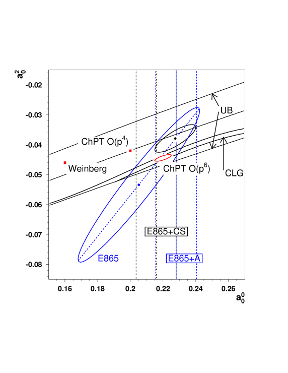
Figure 10: Results for the $\pi\pi$ scattering lengths $a_{0}^{0}$ and $a_{0}^{2}$ obtained from fits to the $K_{e4}$ data directly or from fits to the phase shifts obtained in this experiment. Large ellipse labeled E865: fit to our $K_{e4}$-data leaving both $a_{0}^{2}$ and $a_{0}^{0}$ as free parameters using Eq. 13 with the parameters of ref. ananthanarayan00 (1$\sigma$ contour, see text for remark concerning the region outside the universal band); medium size ellipse without label: fit of ref. descotes02 (1$\sigma$ contour) to our phase shifts; theoretical predictions: weinberg66 (Weinberg, square), gasser83 (ChPT O(p⁴, square), colangelo00 (ChPT O(p⁶, small ellipse); solid curves labeled UB: universal band of allowed values based on Eq. 14; solid curves labeled CLG: narrow band of allowed values based on Eq. 15; solid vertical line labeled E865 (+A $\equiv$ analyticity constraints): fit to $K_{e4}$ data using Eq. 14 with 1 $\sigma$ error limits given by dashed vertical lines; dashed dotted line labeled E865 (+CS $\equiv$ analyticity and chiral symmetry constraints) fit to $K_{e4}$ data using Eq. 15 with 1 $\sigma$ error limits given by dotted vertical lines.

In all previous fits, we have assumed that the decay rate does not depend on $s_{e}$ and that there are no contributions from $p$-waves to $F$. To check this approximation we have allowed these form factors, one at a time, to vary in our fits too for the case where Eq. 14 was used. Table 7 shows that all three form factors are found to be consistent with zero. The nominal values of the contributions to the form factors F and G are at the 2 % or less level. In all three cases, the dominant contribution to the systematic errors came from the resolution of the missing neutrino mass squared, and a smaller non-negligible error from the background estimate.

Parameters	Value	$\chi^{2}/\mbox{ndf}$
$\tilde{f}_{p}$	$-0.34\pm 0.10\pm 0.27\,(-0.02)$	30952/28792
$f_{e}$	$-0.32\pm 0.10\pm 0.24\,(+0.02)$	30954/28792
$g_{e}$	$0.04\pm 0.34\pm 0.88\,(\pm 0.00)$	30963/28792

Table 7: Results from the fits, where the form factors parameters $\tilde{f}_{p}$, $f_{e}$, and $g_{e}$ were allowed to vary one at a time. The quantity in parentheses shows the influence of radiative corrections.

In order to assess the sensitivity of our data to $a_{0}^{2}$ directly we have also made a fit to the data where it was allowed to vary independently, rather then being fixed via Eq. 14 or Eq. 15. The result is given in Table 8 and Fig. 10. While the form factor parameters, as was expected, did not change, $a_{0}^{0}$ shifts to a lower value with a larger error bar, which encompasses the values found above. The error ellipse for this fit is shown in Fig. 10. It illustrates the strong correlation between the two scattering lengths. The long axis of this ellipse follows the equation $a_{0}^{2}=-0.1939+0.6851a_{0}^{0}$.

$f_{s}$	$5.75\pm 0.02\pm 0.08$ (-0.03)
$f_{s}^{\prime}$	$1.06\pm 0.10\pm 0.40$ (+0.37)
$f_{s}^{\prime\prime}$	$-0.60\pm 0.12\pm 0.40$ (-0.37)
$g_{p}$	$4.65\pm 0.48\pm 0.07$ (+0.03)
$g_{p}^{\prime}$	$0.69\pm 0.11\pm 0.04$ ($\pm$ 0.00)
$h_{p}$	$-2.95\pm 0.19\pm 0.20$ (-0.16)
$a^{0}_{0}$	$0.203\pm 0.033\pm 0.004$ (-0.001)
$a^{2}_{0}$	$-0.055\pm 0.023\pm 0.003$ (-0.001)
$\chi^{2}/\mbox{ndf}$	30963/28792

Table 8: Fit of form factor parameterss and scattering lengths $a^{0}_{0}$ and $a^{2}_{0}$. The first error is statistical, the second systematic. The quantity in parentheses shows the influence of the radiative corrections.

VIII Summary and discussion

The main results of this analysis are the measurements of the $\pi\pi$-phase shift difference $\delta$ near threshold and of the form factors $F$, $G$ and $H$ of the hadronic current, and their momentum dependence with a precision which has not been previously attained. We emphasize again, that the analysis based on these data in six bins of invariant $\pi\pi$ mass is model independent.

The analysis which directly relates our data to the scattering length $a^{0}_{0}$, on the other hand, depends on additional input, which leads to slightly different results. While there is a consensus colangelo01b ; colangelo01a ; descotes02 on the use of the Roy-equations ananthanarayan00 and Eq. 13 to relate the phase shifts to the scattering lengths, there exist slightly different ways of linking $a_{0}^{0}$ to $a_{0}^{2}$, and how to make use of peripheral $I=2$ data. These differences produce slightly different results for both $a_{0}^{2}$ and $a_{0}^{0}$ with overlapping statistical errors. The experimental and systematic uncertainities for both the phase shifts and scattering lengths are considerably smaller than the statistical ones and are therefore irrelevant to this discussion.

If both $a_{0}^{0}$ and $a_{0}^{2}$ are allowed to vary independently (Tab. 8), we obtain a result outside the universal band in the $(a_{0}^{0},a_{0}^{2})$ plane, namely

$$a_{0}^{0}=0.203\pm 0.033\ ,\;\;a_{0}^{2}=-0.055\pm 0.023\ .$$

Descotes et al. descotes02 have performed a fit to our published phase shifts pislak01 , which are identical with the ones we give here and obtained

$$a_{0}^{0}=0.237\pm 0.033\ ,\;\;a_{0}^{2}=-0.0305\pm 0.0226\ ,$$

with a strong correlation between the two values, which we also observe in our result. Only that part of the 1$\sigma$ error contour of our result (the large ellipse in Fig. 10) which overlaps the universal band is consistent with both our and the $I=2$ data hoogland74 ; losty74 , and only within this band the solution of the Roy equations ananthanarayan00 used here is valid gilberto02 . From the 1$\sigma$ contour and its central axis we may deduce how much the results listed in Tab. 6 change if the input assumptions on the relation between $a_{0}^{0}$ and $a_{0}^{2}$ are varied. Using the lower limit of the band defined by the bracket in Eq. 14 we find a shift of $a_{0}^{0}$ by $-0.016$, while the maximum allowed upward shift inside the $1\sigma$ contour and the band is $0.012$. Assigning these values as theoretical errors to our result, we obtain

$$a_{0}^{0}=0.228\pm 0.012\;{\rm stat.}\;\pm 0.004\;{\rm syst.}\;^{+0.012}_{-0.016}\;{\rm theor.}$$ (25)

The use of Eq. 14 implies

$$a_{0}^{2}=-0.0365\pm 0.023\;{\rm st.}\;\pm 0.008\;{\rm sy.}\;^{+0.0031}_{-0.0026}\;{\rm th.}$$ (26)

Since the central curve of the universal band is thought to be the best representation of the $I=2$ data, it is no surprise, that the fit of Descotes et al. descotes02 , which used our phase shifts and those of the Geneva-Saclay experiment rosselet77 , Eq. 13 with the parametrisation of Ref. ananthanarayan00 and the $I=2$ data below 800 MeV hoogland74 ; losty74 , gave nearly identical results

$$a_{0}^{0}=0.228\pm 0.012\ ,\;\;a_{0}^{2}=-0.0382\pm 0.0038\ .$$ (27)

This result is also shown in Fig. 8.

Using the narrower band in the $(a_{0}^{2},a_{0}^{0})$ plane defined by Eq. 15 our result is

$$a_{0}^{0}=0.216\pm 0.013\;{\rm st.}\;\pm 0.004\;{\rm sy.}\;{\pm 0.002}\;{\rm th.}\ ,$$ (28)

which implies

$$a_{0}^{2}=-0.0454\pm 0.0031\;{\rm st.}\;\pm 0.0010\;{\rm sy.}\;{\pm 0.0008}\;{\rm th.},$$ (29)

where the theoretical errors have been evaluated as before and correspond to the width of the band. Descotes et al. descotes02 , again fitting to our phase shifts, have obtained for this case

$$a_{0}^{0}=0.218\pm 0.013\ ,\;\;a_{0}^{2}=-0.0449\pm 0.0033\ ,$$ (30)

again in agreement with our result and also with $a_{0}^{0}=0.221\pm 0.026$, obtained by Colangelo et al. colangelo01a by direct numerical inversion of the relation between the phase shifts and the scattering lengths.

From this discussion we may deduce first that using our full data sample or the phase shifts, which we have extracted from it, in the six bins in $M_{\pi\pi}$ leads to the same results. This will make further use of our data easy, should theoretical discussion continue and require this. Second, it has become clear that the most probable values of the two scattering lengths extracted from the $K_{e4}$-data and low-energy $I=2$ data, resting on a minimum of theroretical assumptions given by analyticity and crossing are those given in Eq. 25 and 26, or Eq. 27. Using the additional constraints implied by chiral symmetry and the value of the scalar radius colangelo01a ; colangelo01b leads to a value of the scattering length consistent within the statistical errors with this result, albeit just 1$\sigma$ lower. The authors of Ref. descotes02 have elaborated in detail how their ansatz differs from that of Ref. colangelo01a , and what the possible implications, if any, are for the chiral pertubation theory parameters $\ell_{3}$ and $\ell_{4}$ and the size of the quark condensate. In view of the large errors and also inconsistencies in the $I=2$ phase shift data hoogland74 ; losty74 , it seems premature to assign much significance to this minor discrepancy. Because of the reduced theoretical uncertainties we prefer to quote the values of Eq. 28 and 29 as our final result. Both solutions for $a_{0}^{0}$ are in very good agreement with the full two-loop standard ChPT prediction colangelo00 ; colangelo01b

$a_{0}^{0}=0.220\pm 0.005\ ,\;\;a_{0}^{2}=-0.0444\pm 0.0010\ .$

The influence of the reduced uncertainties of our results on the form factors $F$, $G$ and $H$ on the determination of the low energy constants of ChPT is evident from recent work of Amorós et al. talavera01 , who have updated their earlier work talavera00 using our data pislak01 . The constants $L_{1}^{r}$, $L_{2}^{r}$ and $L_{3}^{r}$ changed from $0.53\pm 0.25$, $0.71\pm 0.27$ and $-2.72\pm 1.12$ (in units of $10^{-3}$), respectively, to $0.43\pm 0.12$, $0.73\pm 0.12$ and $-2.35\pm 0.37$.

The first nonvanishing contribution to the anomalous form factor $H$ in ChPT is predicted to be $H=-2.67$ wess71 . This agrees well with our value of $H=-2.95\pm 0.19\pm 0.20$. An estimation of the next to leading order gives only a small contribution ametller93 .

References

- (1) Now at: Rutgers University, Piscataway, NJ 08855
- (2) Now at: The Prediction Co., Santa Fe, NM 87505
- (3) Now at: Albert-Ludwigs-Universität, D-79104 Freiburg, Germany
- (4) Now at: University of Connecticut, Storrs, CT 06269
- (5) Now at: LIGO/Caltech, Pasadena, CA 91125
- (6) Now at: SCIPP, University of California, Santa Cruz, CA 95064
- (7) E.P. Shabalin, Sov. Phys. (JETP) 17, 517 (1963) (Zh. Eksp. Teor. Fiz. 44, 765 (1963)).
- (8) E.L. Koller et al., Phys. Rev. Lett. 9, 328 (1962).
- (9) L.B. Okun, and E.P. Shabalin, Sov. Phys. (JETP) 10, 1252 (1960) (Zh. Eksp. Teor. Fiz. 37, 1775 (1959)).
- (10) R.W. Birge et al., Phys. Rev. 139, 1600 (1965).
- (11) R.P. Ely et al., Phys. Rev. 180, 1319 (1969).
- (12) W. Schweinberger et al., Phys. Lett. 36B, 246 (1971).
- (13) M. Bourquin et al., Phys. Lett. 36B, 615 (1971); P. Basile et al., Phys. Lett. 36B, 619 (1971); A. Zylberstein et al., Phys. Lett. 38B, 457 (1972).
- (14) E.W. Beier et al., Phys. Rev. Lett. 29, 511 (1972); ibid. Phys. Rev. Lett. 30, 399 (1973).
- (15) L. Rosselet et al., Phys. Rev. D 15, 574 (1977).
- (16) S. Pislak et al., Phys. Rev. Lett. 87, 221801 (2001).
- (17) F. Gomez et al., DIRAC Coll., Proc. Int. Euroconf. on Quantum Chromodynamics: 15 Years of the QCD, Montpellier, France (July 2000), Nucl. Phys. Proc. Suppl. 96, 259 (2001).
- (18) S. Weinberg, Physica 96A, 327 (1979); J. Gasser and H. Leutwyler, Ann. Phys. 158, 142 (1984); Nucl. Phys. B250, 465 (1985).
- (19) For a recent brief overview see e.g. H. Leutwyler, Proc. QCD@Work: Int. Conf. on QCD: Theory and Experiment, Martina Franca, Italy (June 2001), AIP Conf.Proc. 602, 3 (2001); hep-ph/0107332
- (20) Effective field theories of QCD, Proc. 264th WE-Heraeus-Seminar, Bad Honnef, Germany (2001), J. Bijnens, U.G. Meißner, and A. Wirzba eds., hep-ph/201266, and references therein.
- (21) M. Gell-Mann, R.J. Oakes and B. Renner, Phys. Rev. 175, 2195 (1968).
- (22) N.H. Fuchs, H. Sazdjian and J. Stern, Phys. Lett. B269, 183 (1991).
- (23) M. Knecht, B. Moussalam, J. Stern and N.H. Fuchs, Nucl. Phys. B457, 513 (1995); ibid. B471, 445 (1996).
- (24) S. Weinberg, Phys. Rev. Lett. 17, 616 (1966).
- (25) J. Gasser, and H. Leutwyler, Phys. Lett. B125, 325 (1983).
- (26) J. Bijnens et al., Phys. Lett. B374, 210 (1996); Nucl. Phys. B508, 263 (1997); err. ibid. B517, 639 (1998).
- (27) C. Colangelo et al., Phys. Lett. B488, 261 (2000).
- (28) G. Colangelo, J. Gasser, and H. Leutwyler, Nucl. Phys. B603, 125 (2001).
- (29) S.M. Roy, Phys. Lett. 36B, 353 (1971).
- (30) B. Ananthanarayan et al., Phys. Rep. 353/4, 207 (2001).
- (31) M.M. Nagels et al., Nucl. Phys. B147, 189 (1979).
- (32) G. Amorós, J. Bijnens, and P. Talavera, Phys. Lett. B480, 71 (2000); Nucl. Phys. B585, 293 (2000); err. B598, 665 (2001)
- (33) G. Amorós, J. Bijnens, and P. Talavera, Nucl. Phys. B602, 87 (2001).
- (34) For a recent discussion see J. Bijnens, C. Colangelo, G. Ecker, and J. Gasser, Semileptonic kaon decays, hep-ph/9412392, publ. in Ref. daphne95 , p. 315.
- (35) The Second DAPHNE Physics Handbook, L. Maiani, G. Pancheri, and N. Paver eds., INFN-LNF-Divisione Ricerca, SIS-Uffico Publicazioni, (Frascati 1995).
- (36) N. Cabibbo, and A. Maksymowicz, Phys. Rev. 137, B438 (1965).
- (37) A. Pais, and S.B. Treiman, Phys. Rev. 168, 1858 (1968).
- (38) G. Amorós, and J. Bijnens, J. Phys. G25, 1607 (1999).
- (39) K.M. Watson, Phys. Rev.88, 1163 (1952).
- (40) J. Bijnens, Nucl. Phys. B337, 635 (1990).
- (41) C. Riggenbach et al., Phys. Rev. D43, 127 (1991).
- (42) For a review see D. Morgan, and M.R. Pennington, Low energy scattering, publ. in Ref. daphne95 , p. 193.
- (43) D. Morgan, and G. Shaw, Nucl. Phys. B10, 261 (1969).
- (44) A. Schenk, Nucl. Phys. B363, 97 (1991).
- (45) The numerical values for the coefficients are listed in Ref. ananthanarayan00 , appendix D, and Ref. descotes02 , appendix B.
- (46) S. Descotes, N.H. Fuchs, L. Girlanda, and J. Stern, Eur. Phys. J. C24, 469 (2002).
- (47) B. Hyams et al., Nucl. Phys B64, 134 (1973).
- (48) S.D. Protopopescu et al., Phys. Rev. D7, 1279 (1973).
- (49) G. Colangelo, J. Gasser, and H. Leutwyler, Phys. Rev. Lett. 86, 5008 (2001).
- (50) R. Appel et al., Nucl. Instr. Meth. A479, 349 (2002).
- (51) G.S. Atoyan et al., Nucl. Instr. Meth. A320, 144 (1992).
- (52) D.E. Groom et al., Eur. Phys. J. C15, 1 (2000); K. Hagiwara et al., Phys. Rev. D66 (2002) 010001.
- (53) A.M. Diamant-Berger, Étude expérimentale a haute statistique de la désintégration du meson dans le mode et analyse des paramétres qui gouvernent cette désintégration, Ph.D. thesis, University of Paris, Orsay; Centre d’Etudes Nucléaires de Saclay, 1976, report CEA-N-1918, unpublished.
- (54) see T.G. Trippe, in Ref. groom00 , p. 503.
- (55) K.O. Mikaelian, and J. Smith, Phys. Rev. D5, 1763 (1972).
- (56) R. Brun et al., GEANT 3.21, CERN Geneva.
- (57) R. Appel et al., Phys. Rev. Lett. 83, 4482 (1999); H. Ma et al., Phys. Rev. Lett. 84, 2580 (2000).
- (58) W.T. Eadie et al., Statistical Methods in Experimental Physics, (North Holland, Amsterdam and London, 1971).
- (59) G.D. Lafferty and T. R. Wyatt, Nucl. Instr. Meth. A355, 541 (1995).
- (60) see Ref. diamant76 , appendix 2.
- (61) A. Neveu, and J. Scherk, Phys. Lett. 27B, 384 (1968).
- (62) A. Alavi-Harati et al., Phys. Rev. D64, 112004 (2001).
- (63) F. Low, Phys. Rev. 110, 974 (1958).
- (64) W. Hooogland et al., Nucl. Phys. B69, 266 (1974); ibid. B126, 109 (1977).
- (65) M.J. Losty et al., Nucl. Phys. B69, 185 (1974).
- (66) We thank G. Colangelo for pointing this out.
- (67) J. Wess and B. Zumino, Phys. Lett. 37B, 95 (1971).
- (68) L. Ametller et al., Phys. Lett. B303, 140 (1993).