Interpolating the Free Energy Density Differences of reweighting methods

Abstract

A discussion of the overlap problem of reweighting approaches to evaluating critical phenomenon in fermionic systems is motivated by highlighting the divergence of the joint probability density function of a general ratio. By identifying the bounds for which this integral can be expressed in closed form, we establish criteria for accurately mapping the joint ratio distribution of two disjoint ensembles through interpolation. The approach is applied to QCD with four staggered flavours to evaluate the critical line in the $\beta-\mu$ plane.

1 Introduction

The pathology of fermionic reweighting schemes can be succinctly expressed in the free energy density difference, $\Delta f$, given by the ratio of two partition functions for a given finite system of intensive and extensive variables, $\beta$, and, $V$. Reweighting methods attempt to effect this difference through numerical simulation by normalising observables with the ratio of the Monte Carlo functional measures for the two separate ensembles.

$$\frac{\Omega}{\Omega^{\prime}}=exp\{\,-\Delta f\,\,\beta V\,\}$$ (1)

However, as the free energy density difference that can be evaluated is necessarily positive the exponent of this ratio can become vanishingly small. The relevance of the ensemble that can be numerically evaluated, $\Omega^{\prime}$, to the phase space of the ensemble of interest, $\Omega$, therefore becomes questionable. Simple-mindedly we could ask how close two ensembles must be for a reweighting measurement to be unaffected by this finite difference.

2 Probability Density Function of a Ratio

This question can be expressed in general terms through the joint probability density function, $\phi_{\frac{A}{B}}(t)$, of the ratio of two normally distributed variables, $x$, and, $y$. Both having a given mean, $\mu\,$, and variance, $\sigma$, and in the following example below vanishing probability densities everywhere but for positive values of $y$ and $x$.

$$t=\frac{y}{x}\,\,\,\,\,\,\,\,\,\,\,\,\,y:\phi_{A}(\mu_{A},\sigma_{A})\,\,\,\,\,\,\,\,\,\,x:\phi_{B}(\mu_{B},\sigma_{B})$$ (2)

$$d\phi_{\frac{A}{B}}(t) = \int_{x=0}^{\infty}dx\ \phi_{A}(tx).\phi_{B}(x)\int_{y=tx}^{(t+dt)x}dy$$ (3)

$$\phi_{\frac{A}{B}}(t)=\lim_{dt\rightarrow 0}\frac{d\phi_{\frac{A}{B}}(t)}{dt} = \int_{x=0}^{\infty}\,\,dx\,\,x\,\,\phi_{A}(tx).\phi_{B}(x)$$ (4)

$$=\frac{\sigma_{A}^{2}\mu_{B}t+\sigma_{B}^{2}\mu_{A}}{\sqrt{2\pi}(\sigma_{A}^{2}t^{2}+\sigma_{B}^{2})^{3/2}}exp\left\{-\frac{(\mu_{B}-\mu_{A}t)^{2}}{2(\sigma_{B}^{2}+\sigma_{A}^{2}t^{2})}\right\}$$ (5)

Even for this overly simplistic case the joint probability density function of the ratio has a nonzero Cauchy component and so all higher moments (including the mean and variance) are undefined. Insight is gained with the central limit theorem under Lyapunov conditions [1], where the distribution of the ratio will asymptotically approach normal if the mean of the ratio is several standard deviations from zero. Similarly, under these conditions the higher moments can thus be properly defined for the discrete finite free energy density distribution of Eq. (1) which relates to the pathology of reweighting [2].

$$\left\langle{{\mathcal{O}}}\right\rangle_{\beta} = \frac{\sum_{i}^{N}{\mathcal{O}}e^{-\Delta\beta E_{i}}}{\sum_{i}^{N}e^{-\Delta\beta E_{i}}}$$ (6)

$$\{{\mathcal{O}}\}=\frac{1}{N}\sum_{i}^{N}{\mathcal{O}}(E_{i}) e^{-\Delta\beta E_{i}} \,\,\,\,\,\,\,\,\,\,\,\,\,\,\{{\mathcal{O}},1\}=\frac{1}{N}\sum_{i}^{N}{\mathcal{O}}(E_{i})e^{-2\Delta\beta E_{i}}$$ (7)

$$\frac{(\delta{\mathcal{O}})^{2}}{{\left\langle{{\mathcal{O}}}\right\rangle_{\beta}}^{2}} = \left(\frac{\{{\mathcal{O}},{\mathcal{O}}\}}{\{{\mathcal{O}}\}^{2}}-1\right)\,\,+\,\,\left(\frac{\{1,1\}}{\{1\}^{2}}-1\right)\,\,-\,\,2\left(\frac{\{{\mathcal{O}},1\}}{\{{\mathcal{O}}\}\{1\}}-1\right)$$ (8)

Ignoring the integrated autocorrelation times of the Monte Carlo evaluation in the above defintion the relative error of a reweighted observable $\left\langle{{\mathcal{O}}}\right\rangle_{\beta}$ is clearly minimised for when the observable ${\mathcal{O}}$ approaches unity. Conversely, if an observable is normalised so that the mean is unity with a small standard deviation, we have ensured that Lyapunov-type conditions are valid (at least for the numerator). Since with reweighting a measurement can be redefined relative to a different ensemble simply by explicitly evaluating a free energy density difference in the measurement, the remaining denominator can be expressed as the product of a series of terms each incrementally close to unity. It is then straightforward to show with Eq. (8) that the relative error of such a product converges with an increasing number of increments for the given ${\mathcal{O}}$ factored in this manner. By expressing the free energy density difference of Eq. (1) as the product of series of vanishingly small differences under appropriate contraints the finite free energy density difference of reweighting can thus be interpolated.

3 Sign Problem

The importance sampling evaluation procedure of a Monte Carlo method is essentially undefined for non-positive definite weights. This is the case for spin systems such as the Hubbard model where one effective measure which is used for simulations is the modulus ensemble [3].

$$\left\langle{\mathcal{O}}\right\rangle=\frac{\int DU\,\,{\mathcal{O}}\,\,{\rm{det}M}e^{-S}}{\int DU\,\,{\rm{det}M}e^{-S}}$$ (9)

$${\rm{det}M\,\,\,is\,\,\,real,}\,\,\,\,\,\,\,\,\,\,\,\,sgn({\rm{det}M})=\left\{\begin{array}[]{c}-1\\ +1\end{array}\right.$$ (10)

$$\left\langle{\mathcal{O}}\right\rangle_{\|} = \frac{\int DU\,\,{\mathcal{O}}\,\,{\|\rm{det}M\|}e^{-S}}{\int DU\,\,{\|\rm{det}M\|}e^{-S}}$$ (11)

$$\left\langle{\mathcal{O}}\right\rangle = \frac{\left\langle\,{\mathcal{O}}.sgn({\rm{det}M})\,\right\rangle_{\|}}{\left\langle\,sgn({\rm{det}M})\,\right\rangle_{\|}}$$ (12)

To interpolate $sgn({\rm{det}M})$ we would therefore rewrite the ratio of expectations in Eq. (12) as a product of expectations of increments close to unity. Bringing the numerator into a similar product form as the denominator if required by a significant probability density of the numerator at zero.

$$\frac{\mathcal{O}}{\mathcal{O}_{o}}\sim 1\,\,\,\,\,\,\,\,\,\,\,\,\,\,\,\,\,\,\,\,\,{\mathcal{O}_{o}}\,-1=N\delta$$ (13)

$$\left\langle{\mathcal{O}}\right\rangle = \frac{\left\langle\frac{\mathcal{O}}{\mathcal{O}_{o}}\,.\,sgn({\rm{det}M})\,\right\rangle_{\|}}{\prod_{n=1}^{N}Re\left\langle\frac{1+\delta(n-1)}{1+\delta n}\,.\,exp\left\{\,\frac{i\pi}{2N}(1+sgn({\rm{det}M}))\,\right\}\,\right\rangle_{\|}}$$ (14)

4 Overlap Problem

Following the inclusion of the chemical potential $\mu$ into the fermionic action, lattice QCD is similarly unamenable to direct Monte Carlo treatment as ${\rm{det}M(\mu)}$ is complex valued for $\mu\neq 0$. A case in point is the finite density Glasgow method [4]. The distribution of a set of normalised expansion coefficients is wanted at a point on the critical line, $\mu_{1}$, but an ensemble can only be generated on the real line for $\mu_{o}=0$. We may now, though, express the relation between the two normalised ensemble-averaged expansion terms for these two regions ($\mu_{1},\mu_{o}$) in terms analogous to the sign/modulus relation defined for the sign problem in Eq. (14).

$$\left\langle{\frac{{c_{n}}}{{\rm{det}}M(\mu_{1})}}\right\rangle_{\mu_{1}}\longleftrightarrow\left\langle{\frac{{c_{n}}}{{\rm{det}}M(\mu_{o})}}\right\rangle_{\mu_{o}}\,\,\,\,\,\,\,\left\langle{\mathcal{O}}\right\rangle\longleftrightarrow\left\langle{\mathcal{O}}\right\rangle_{\|}$$ (15)

$$\left\langle{\frac{{c_{n}}}{{\rm{det}}M(\mu_{1})}}\right\rangle_{\mu_{1}}=\frac{\left\langle{\frac{c_{n}}{{\rm{det}}M(\mu_{1})}\frac{{\rm{det}}M(\mu_{1})}{{\rm{det}}M(\mu_{o})}}\right\rangle_{\mu_{o}}}{\left\langle{\frac{{\rm{det}}M(\mu_{1})}{{\rm{det}}M(\mu_{o})}}\right\rangle_{\mu_{o}}}$$ (16)

As before to accurately map the free energy density difference between ensembles a normalising factor is inserted to bring the numerator close to unity and the remaining free energy density difference is interpolated in the denominator.

$$\left\langle{\frac{{c_{n}}}{{\rm{det}}M(\mu_{1})}}\right\rangle_{\mu_{1}} = \frac{\left\langle{\frac{c_{n}}{{\rm{det}}M(\mu_{0})}\frac{1}{{\rm{det}}M(\mu_{2})}}\right\rangle_{\mu_{o}}}{\left\langle{\frac{{\rm{det}}M(\mu_{1})}{{\rm{det}}M(\mu_{0})}\frac{1}{{\rm{det}}M(\mu_{2})}}\right\rangle_{\mu_{o}}}$$ (17)

$$=\frac{\left\langle{\frac{c_{n}}{{\rm{det}}M(\mu_{3})}}\right\rangle_{\mu_{o}}}{\left\langle{\frac{{\rm{det}}M(\mu_{1})}{{\rm{det}}M(\mu_{3})}}\right\rangle_{\mu_{o}}} = \frac{\left\langle{\frac{c_{n}}{{\rm{det}}M(\mu_{3})}}\right\rangle_{\mu_{o}}}{\prod_{n=1}^{N}\left\langle{\frac{{\rm{det}}M(n\Delta\mu)}{{\rm{det}}M(\,[n+1]\Delta\mu\,)}}\right\rangle_{\mu_{o}}}$$ (18)

$$\frac{c_{n}}{{\rm{det}}M(\mu_{o}){\rm{det}}M(\mu_{2})}=\frac{c_{n}}{{\rm{det}}M(\mu_{3})}\sim 1\,\,\,\,\,\,\,\,\,\,\,\,\,\,\,\frac{{\rm{det}}M(\mu_{1})}{{\rm{det}}M(\mu_{3})}={\rm{det}}M(N\Delta\mu)$$ (19)

For convenience, rather than determine the normalised distributions at the critical line from ensembles generated for several $\beta$ values we additionally reweight in $\beta_{1}$. The modified coefficient being again normalised to unity through a choice for $\mu_{3}$.

$$c_{n}\rightarrow c_{n}\,.\,exp\{-S_{g}(\beta_{1})+S_{g}(\beta_{o})\}$$ (20)

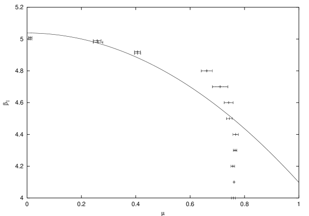
Figure 1: The critical line in the $\beta_{1}-\mu$ plane for $n_{f}=4$ QCD, determined from the zeros of a fugacity polynomial expansion.

The zeros of this polynomial which approach the real axis of the expansion variable in the thermodynamic limit identify the critical line [5]. A preliminary critical value for $\mu$ is plotted as a function of $\beta_{1}$ in Figure 1. It should be noted that since the polynomial is deflated during rootfinding there is no actual dependence on the transition value of $\mu_{1}$, and consequentially no need to tune the reweighting parameters to effect cancellations through the covariance. The above ensemble consists of 2,000 configurations on a $4^{4}$ volume at $\beta_{o}=5.04$ with $m=0.10$, though strictly the quadratic fit [6] is for a smaller bare mass $(m=0.05)$. The congruence is therefore qualitative, although the fall-off at $\mu\sim 0.7$ [7] is perhaps more consistent with expectations for the density of nuclear matter at $\beta_{1}=0.0$.

References

[1] O. Kallenberg,
Foundations of Modern Probability, Springer (2002).
[2] A. M. Ferrenberg, et al,
Phys. Rev.E557, 5092 (1995).
[3] S. Chandrasekharan and U. -J. Wiese,
Phys. Rev. Lett.83, 3116 (1999).
[4] P. E. Gibbs, Phys. Lett.B172, 53 (1986);
I. M. Barbour and A. J. Bell, Nucl. Phys.B372, 385 (1992).
[5]
C.N. Yang and T.D. Lee, Phys. Rev.87, 404 (1952).
[6]
M. D’Elia and M. -P. Lombardo, hep-lat/0209146.