Measurement of $CP$ Asymmetries at Belle

Abstract

The Belle experiment at the KEK $B$ factory has collected 93 fb^-1 of electron positron collisions at $\sqrt{s}=10.6$ GeV. This has produced a sample of 85 million $B{\bar{B}}$ meson pairs that can be used to study $CP$ violation in rare (and not so rare) $B$ decay modes. Here I report on a measurement of indirect $CP$ violation in the decay $B^{0}\rightarrow J/\psi K^{0}_{S}$, as well as time dependent $CP$ asymmetries in rarer modes such as $B^{0}\rightarrow\pi^{+}\pi^{-},\eta^{\prime}K_{S}^{0}$ and $\phi K^{0}_{S}$. I summarise the prospects for improving the precision on these and related measurements.

1 $CP$ Violation in $B$ Decay

When $CP$ violation was first observed in neutral kaon decay, in the early 1960s, it shook the foundations of particle physics. It had previously been assumed that the combination of charge conjugation and a parity transformation left all known particle interactions invariant, despite the fact that weak interactions violated parity alone. Over the following three decades $CP$ violation in the $K^{0}$ system was measured with ever increasing precision in an attempt to pin down its source. In the 1970s Kobyashi and Maskawa [1] showed that the Standard Model could accommodate $CP$ violation in a three quark weak mixing matrix, $V_{\rm CKM}$. The single non-trivial phase in such a $3\times 3$ unitary matrix could explain the small effect first seen in $K^{0}$ meson decay, where $CP$ violation was observed at the $10^{-3}$ level. It was suggested [2], in the early 1980s, that the comparable amplitudes for the direct decay of $B^{0}$ mesons into $CP$ eigenstates and the mixing of $B^{0}{\bar{B}^{0}}$ mesons would make neutral $B$ meson decay an ideal place to observe large indirect $CP$ violating effects.

One way to understand the magnitude of $CP$ violation predicted by the CKM model, in neutral $B$ meson decay, is to consider the unitarity relation between the first and third columns of $V_{\rm CKM}$:

$$V_{tb}^{*}V_{td}+V_{cb}^{*}V_{cd}+V_{ub}^{*}V_{ud}=0.$$

While each term in this expression is relatively small (${\cal O}(\sin^{3}\theta_{C})$), they are all the same size. When plotted in the complex plane (see fig. 1) one expects significant angles at each apex because the sides of the triangle have similar lengths. In neutral kaon decay the corresponding unitarity triangle has two sides that are much larger than the third – making the decay rates for $K^{0}$ mesons much larger, but making the angles, and hence the observable phases small and more challenging to measure.

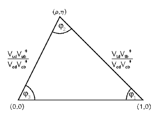
Figure 1: Unitarity of the CKM matrix relates its different elements. The study of $CP$ violation in $B$ meson decay involves the CKM elements depicted in this triangular relationship.

In $B$ meson decay $CP$ violating phases are most readily observed through the indirect mixing of two amplitudes. Given a $CP$ eigenstate accessible to both $B^{0}$ and ${\bar{B}^{0}}$ decays – such as $J/\psi K^{0}_{S}$ – one can observe the interference between the direct decay amplitude for:

$$B^{0}({\bar{B}^{0}})\rightarrow J/\psi K_{S}^{0};$$

and the amplitude for the same decay preceded by $B^{0}$ mixing:

$$B^{0}({\bar{B}^{0}})\rightarrow{\bar{B}^{0}}(B^{0})\rightarrow J/\psi K_{S}^{0}.$$

When one includes the relative phase between these two amplitudes we get an expression for the time dependent $CP$ asymmetry:

$A_{CP}(\Delta t)$	$\equiv$	${{{dN\over dt}(\bar{B^{0}}\rightarrow J/\psi K_{\xi})-{dN\over dt}(B^{0}\rightarrow J/\psi K_{\xi})}\over{{dN\over dt}(\bar{B^{0}}\rightarrow J/\psi K_{\xi})+{dN\over dt}(B^{0}\rightarrow J/\psi K_{\xi}}}$,
	=	- $\xi_{K}\sin~{}2\phi_{1}\>\sin~{}\Delta m\Delta t.\qquad\qquad[1]$

Where the asymmetry in the decay rate between $B^{0}$ and ${\bar{B}^{0}}$ mesons is proportional to the $B^{0}$ mixing rate ($\sin\Delta m\Delta t$), the $CP$ eigenvalue of the final state, $\xi_{K}$, ($\xi_{K}=-1$ for $J/\psi K^{0}_{S}$ and +1 for $J/\psi K^{0}_{L}$) and $\sin 2\phi_{1}$, the angle at the lower right apex of the unitarity triangle shown in fig. 1.

2 The KEK-B Collider and Belle Detector

The main experimental challenge in measuring $CP$ violation in $B^{0}$ meson decay lies in the fact that $B^{0}$ mesons decay much more quickly than $K^{0}$ mesons, having proper flight distances of fractions of a millimeter. Furthermore the decay rate to experimentally accessible $CP$ eigenstates are much smaller, on the order of ${\cal O}(10^{-4})$ for $B^{0}$ mesons; while essentially 100% of $K^{0}$ meson decays are to identifiable $CP$ eigenstates. While the very much larger $CP$ violation in $B^{0}$ decay makes up for some of this it remained a significant experimental challenge to observe $CP$ violation in $B^{0}$ meson decay.

The key ingredient is having a high luminosity source of $B$ mesons – a $B$ factory. Two dedicated machines were built in the late 1990s to address this. The KEK-B $e^{+}e^{-}$ accelerator complex collides beams of 8 GeV electrons and 3.5 GeV positrons, to produce $\Upsilon(4S)$ mesons at $\sqrt{s}=10.6$ GeV. These, in turn, decay into $B{\bar{B}}$ meson pairs. Using an 11 mrad crossing angle KEK-B is able to collide beams with currents in excess of 1 Ampere, with tolerable backgrounds and luminosities approaching $10^{34}$ per cm² each second. An integrated luminosity comparison between the KEK-B factory and its competitor, PEP-II at SLAC, is shown in fig. 2. While the two machines have delivered similar integrated luminosities since they came online two years ago, the recent instantaneous luminosities (the slope of the curve) in the KEK machine bodes well for upcoming data-taking.

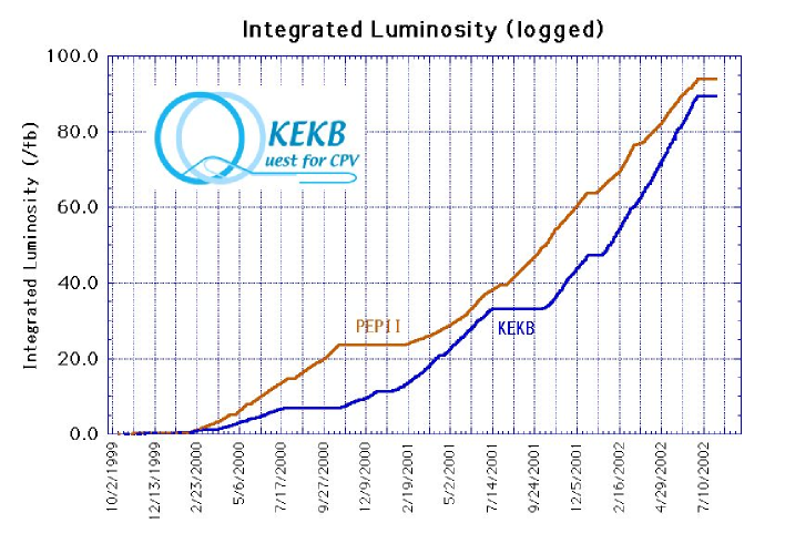
Figure 2: The Belle experiment has been collecting data over the last two years. This plot shows the integral luminosity over that period (lower line) compared to the luminosity collected by the BaBar experiment at PEPII (upper line). The data samples are similar at this point.

The colliding beam energies are asymmetric so that the $\Upsilon(4S)$ meson produced is boosted along the beam direction. This results in the daughter $B$ mesons also being boosted, with $\beta\gamma\approx 0.45$, separating the two $B$ meson decay vertices in the detector. The boost introduces some asymmetry in the design of the experiment. A cross-section of the cylindrical Belle detector is shown in fig. 3. The detector elements are arranged asymmetrically around the interaction point to increase the acceptance for $B$ meson decay products.

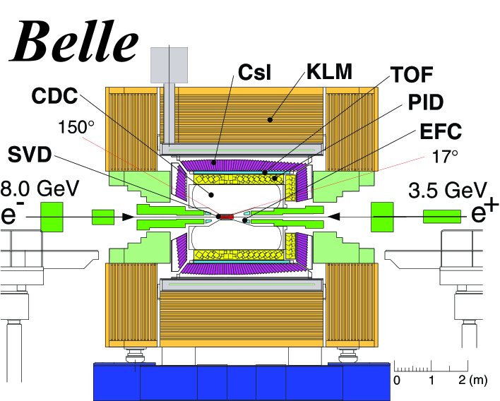
Figure 3: An elevation view of the Belle experiment.

Working outwards from the collision point $B$ meson decay products encounter a three layer silicon vertex detector (SVD) that measures charged particle trajectories with 55 $\mu$m precision (at 1 GeV/c) and the separation of $b$ decay vertices with a precision of 100 $\mu$m in $z$. They next pass through a Helium filled drift chamber (CDC) that measures track momenta with a precision of $\sigma_{p}/p=(0.2p\oplus 0.3)\%$ ($p$ measured in GeV/c) providing excellent mass resolution for $B$ decays into charged daughter tracks. This is followed by a Cesium-Iodide crystal calorimeter (CsI) that has better than 2% energy resolution for 1 GeV photons. Belle’s particle identification system includes an aero-gel Cerenkov counter system (PID) and a time of flight system (TOF) that can distinguish kaons from pions up to 3.5 GeV/c with 90% efficiency and fake rates of less than 5%. These systems are followed by the solenoid coil and then a $K^{0}_{L}$ and muon detection system (KLM) that identifies muons with less than 2% fake rate above 1 GeV/c. As a hadron absorber it also detects $K_{L}^{0}$ showers with an angular resolution of a few degrees.

The Belle detector has operated reliably over the first two years of KEK-B operation, accumulating 78 fb^-1 on the $\Upsilon(4S)$ resonance corresponding to 85 million $B{\bar{B}}$ pairs that can be used to study $CP$ violation in $B^{0}$ decay [3].

3 The Measurement of $\sin 2\phi_{1}$

There are three main ingredients that go into the measurement of a $CP$ phase – for example $\sin 2\phi_{1}$ in $J/\psi K_{S}^{0}$ decay – at Belle. These are illustrated in fig. 4. First, one must identify the decay vertices of the two $B$ mesons. Second, since the final state under study is a $CP$ eigenstate, we must tag the flavour of one $B$ meson when it decays. Since the $\Upsilon(4S)$ decay products evolve in a coherent $J=1$ state, the decay of one of the $B$ mesons into a $B^{0}$ (in the example shown in fig. 4) projects the other $B$ meson into a known ${\bar{B}^{0}}$ state. Finally, one must identify a sample of candidates which are $CP$ eigenstates – for example $J/\psi K^{0}_{S}$ decays. I will briefly describe each of these aspects of the measurement in the following sections.

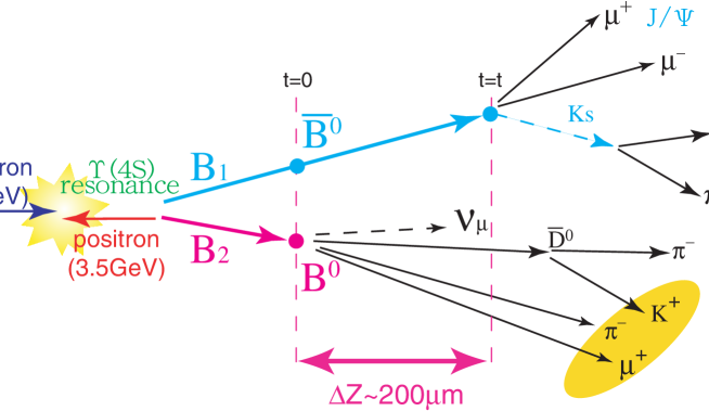
Figure 4: A schematic view the ingredients necessary to observe $CP$ violation in $B$ meson decay at an asymmetric $e^{+}e^{-}$ collider.

3.1 $B$ Meson Decay Vertexing

Identifying and separating the two $B$ decay vertices on an event-by-event basis in Belle is a subtle process. Despite the boost from the asymmetric beam energies the $B$ mesons only travel a few hundred microns ($\gamma c\tau\approx 200\mu$m) on average before they decay. The silicon vertex detector in Belle measures the decay vertices with a precision of about 100 $\mu$m. A $J/\psi K^{0}_{S}$ decay vertex is typically determined with a precision of 75 $\mu$m, slightly better than the flavour tag $B$ decay, which has a precision of 140 $\mu$m, because there are generally more reconstructed tracks attached to the former vertex.

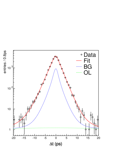
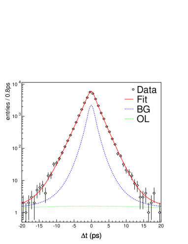
Figure 5: Left: The distribution of decay time differences for $B^{0}$ and ${\bar{B}^{0}}$ mesons measured by Belle. The open circles are the data, the solid line is the result of a maximum likelihood fit that includes a component proportional to the lifetime, and two components (dashed and dotted) that parametrise the detector resolution. Right: The distribution of decay time differences for $B^{+}$ and $B^{-}$ mesons.

The precision of Belle’s vertexing is demonstrated by its $B$ lifetime measurements (shown in fig. 5) where one sees a clear difference between the detector resolution (dashed line) and the longer lived $B$ meson decays (solid line through the data points). These fits give precise measurements of the charged and neutral $B$ meson lifetimes and their ratio: $\tau_{+}/\tau_{0}=1.09\pm 0.03$ [4]. The detector resolution is understood out to ten $B$ lifetimes and over three orders of magnitude in $B$ decay rate. This is one of the crucial ingredients to measuring $CP$ violation.

3.2 Flavour Tagging in $B^{0}$ Meson Decay

A second key ingredient is being able to tag the flavour of the $B$ meson accompanying the $CP$ eigenstate in the $B{\bar{B}}$ decay. This is done without fully reconstructing the opposite $B$ – which would result in a significant loss in efficiency. Instead we look for characteristics of the other $B$ decay that tag its flavour. For example, high momentum leptons indicate a direct semi-leptonic $B$ decay, where the charge of the lepton is determined by the flavour of $B$. Lower momentum leptons arise from cascade semi-leptonic decays where the $B$ meson first decays to a charmed meson and the latter decays semi-leptonically. This results in the opposite correlation between the lepton charge and $B$ meson flavour. Such information is combined in a set of look-up tables shown in fig. 6 that classify potential flavour information according to the sign of the $b$ quark charge, $q$, and the reliability of the tagging information, $r$.

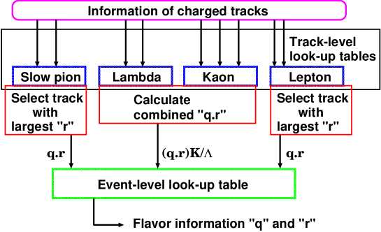
Figure 6: A schematic view of the Belle $B$ flavour tagging algorithm. Events are classified by the following characteristics: charged leptons, kaons, lambdas and slow pions. This information is sifted through a set of look-up tables (based on Monte Carlo simulation) to identify and quantify the most reliable flavour tagging information in each event. The result of this procedure is the assignment of a “charge”, $q$, and the reliability, $r$, of the flavour assignment.

While the look-up table information: $q$, $r$ and their correlations – when more than one piece of tagging information is available in a single event – is extracted from a Monte Carlo simulation, the efficiency of the tagging algorithm is calibrated on a data control sample. Using a sample of $B\rightarrow D^{*}l\nu$ decays – where one knows the flavour of the $B$ meson from the charge of the lepton in the final state – the $B$ mixing parameter is measured from the time-dependence of the observed decays. We use our flavour tagging algorithm, described above, to classify events into six different ranges of $r$, shown in fig. 7. One sees that the observed amplitude of the mixing oscillation is much less in the sample tagged with lowest reliability (top left) while the amplitude of the oscillation (at $\Delta t=0$) almost reaches 1 for those events that our algorithm tags with the highest reliability (bottom right).

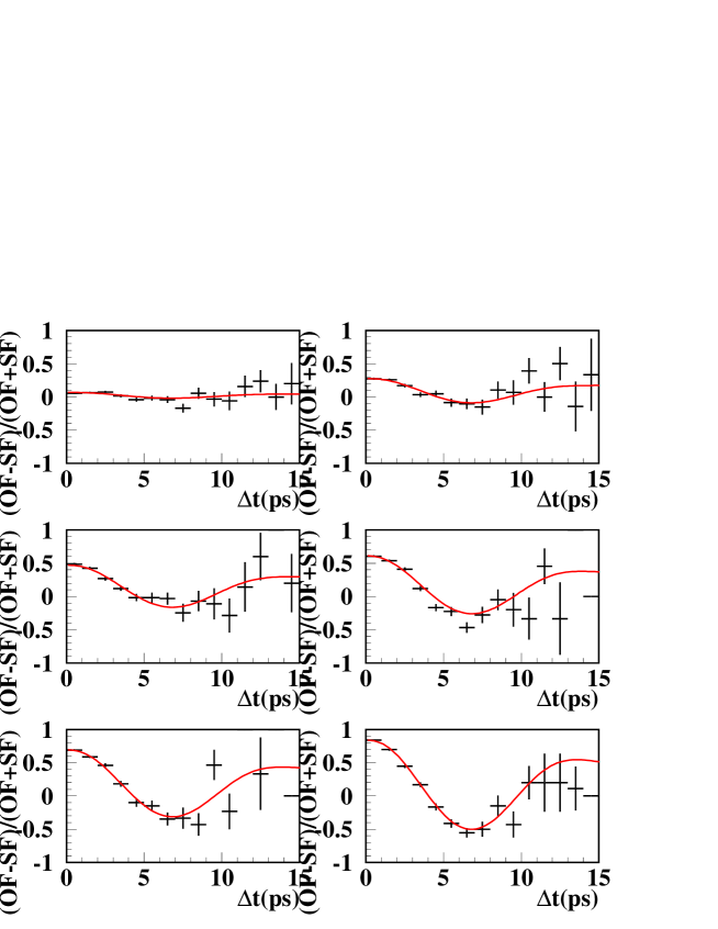
Figure 7: $B$ mixing measurements in self-tagged $B^{0}\rightarrow D^{*+}l^{-}\nu$ samples. This sample calibrates our tagging efficiency. The amplitude of the mixing observed, hence the efficiency of our tagger, depends on the reliability of the tag, which increases from top-left to bottom-right in this series of plots.

Figure 8 shows the correct tag probability from the six plots in fig. 7 versus the average $r$ for each sample. The correct tag probability, $1-2w_{l}$, is extracted from $w_{l}$ – the probability that a tag gives the wrong charge sign. In cases were $w_{l}$ approaches 0.5 (a 50-50 guess at the charge of the $b$ quark) the probability of correctly tagging the flavour of the $B$ meson goes to 0. Conversely, when $w_{l}$ goes to 0, one approaches a 100% correct tag probability. Figure 8 shows a strong correlation between our tagger’s reliability, $r$, and the correct tag probability as measured in our control sample. These measured tag probabilities are used to weight the $CP$ eigenstate decays in the fit to extract their decay asymmetry.

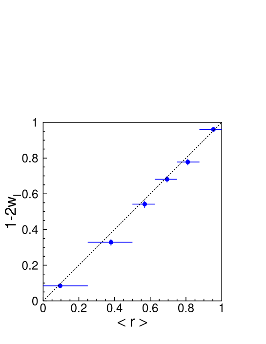
Figure 8: The correct tag probability ($1-2w_{l}$) versus tag reliability, $r$. The wrong-tag fraction ($w_{l}$) is measured from the observed mixing in self-tagged $B^{0}$ samples (see fig. 7). The measured tagging probabilities ($1-2w_{l}$) are used to weight the flavour determination in fits to $CP$ eigenstates.

With this algorithm we extract some tagging information from 99.5% of all $B$ decay candidates in Belle. While some of the events have tags with low reliability, we measure an overall tagging efficiency of $28.8\pm 0.6\%$, corresponding to almost 1/3 of our $B$ sample being perfectly tagged. This represents an improvement from an effective tagging efficiency of $27.7\pm 1.2\%$ in previous measurements [3] arising from an increase to our low-momentum track reconstruction efficiency and an improved silicon alignment – allowing us to associate more tracks with the tagging $B$ decay vertex. The reduced uncertainty on our tagging efficiency is the result of tripling of the size of the control data sample.

3.3 $CP$ Eigenstate Event Samples

From 78 fb^-1 of data taken at the $\Upsilon(4S)$ resonance Belle has identified a sample of almost 3000 $B^{0}\rightarrow c{\bar{c}}K$ decay candidates. These are summarised in table 1 where one sees that a little over 1/3 of the candidates come from $J/\psi K^{0}_{S}$ decays where the $K^{0}_{S}$ is reconstructed in a $\pi^{+}\pi^{-}$ final state. This golden mode also has the highest purity. We also have a number of other modes that are used to measure $\sin 2\phi_{1}$ with other $c{\bar{c}}$ resonances and other $K^{0}_{S}$ final states. Finally, about $40\%$ of our sample is in the form of $J/\psi K_{L}^{0}$ decays that have the opposite $CP$ eigenvalue. This sample provides an important cross-check for possible $CP$ dependent systematic effects in our measurement. Figure 9 shows the mass distribution for our candidates with $K^{0}_{S}$ candidates in the final state.

Mode	CP ($\xi_{K}$)	Candidates	Purity (%)
$J/\psi K_{S}^{0}(\pi^{+}\pi^{-})$	-1	1116	98
$J/\psi K_{S}^{0}(\pi^{0}\pi^{0})$	-1	162	82
$\psi(2S)K_{S}^{0}$	-1	172	93
$\chi_{c1}K_{S}^{0}$	-1	67	96
$\eta_{c}K_{S}^{0}$	-1	122	68
$J/\psi K^{*0}(K_{S}^{0}\pi^{0})$	1 (81%)	89	92
$J/\psi K_{L}^{0}$	1	1230	63
Total		2958

Table 1: Summary of the $CP$ candidates, after flavour tagging and decay vertexing, used to measure $\sin 2\phi_{1}$.

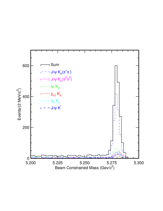
Figure 9: The beam constrained mass for the different $B^{0}\rightarrow{\bar{c}}cK_{S}^{0}$ final states used to measure indirect $CP$ violation in Belle. The largest sample comes from the $J/\psi K^{0}_{S}(\pi^{+}\pi^{-})$ decays (dot-dashed line). The other modes combine to make up about 20% of our sample (see table 1).

While our $K_{L}^{0}$ detector does not measure the energy of the hadronic shower of a neutral Kaon decay with high precision, it does measure the shower direction with an accuracy of a few degrees. Having fully reconstructed a $J/\psi$ meson one can hypothesize that a $B^{0}\rightarrow J/\psi K_{L}^{0}$ decay has occurred and infer the magnitude of the $K_{L}^{0}$ momentum using only the $K_{L}^{0}$ direction, by constraining the two body system ($J/\psi$, $K_{L}^{0}$) to have the $B^{0}$ mass. Imposing this constraint reduces the number of handles one has to reject background but still provides one degree of freedom – chosen to be the momentum of the $B^{0}$ candidate in $\Upsilon(4S)$ centre of momentum (shown in fig. 10). Successfully reconstructed $J/\psi K_{L}^{0}$ candidates peak near $p_{B}^{\rm cms}\approx 0.3$ GeV/c, while backgrounds generate a flatter distribution in $p_{B}^{\rm cms}$. From the distribution in fig. 10 we extract 1330 candidate events (before flavour tagging or decay vertex reconstruction) and estimate their purity to be 63%. Since many of the backgrounds under the $J/\psi K_{L}^{0}$ peak result from other $B$ meson decays care must be taken when extracting a $CP$ asymmetry from this sample to account for the $CP$ asymmetry of the background. We do this with Monte Carlo studies whose ability to constrain the $CP$ content of the background is reflected in a systematic uncertainty on $\sin 2\phi_{1}$ from this channel.

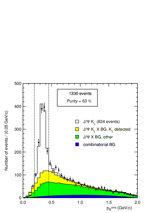
Figure 10: The centre of mass momentum distribution for Belle’s $J/\psi K_{L}^{0}$ candidates used to measure indirect $CP$ violation. The signal forms a peak at $p_{B}^{\rm cms}=0.33$ GeV/c, while backgrounds – where one or more final state particles have not been included in the $B^{0}$ candidate reconstruction – have their momentum smeared out.

3.4 Results

We perform a maximum likelihood fit to all our $B^{0}\rightarrow c{\bar{c}}K$ candidates to extract their time dependent asymmetry (as shown in eqn. 1). This fit includes the flavour tagging probability, uncertainties on the measured separation between the two $B$ meson decays (converted to $\Delta t$ using the $B$ meson boost) as well as the purity of the signal for each type of decay. The $J/\psi K_{S}^{0}(\pi^{+}\pi^{-})$ candidates receive the highest weight because they have much smaller backgrounds (see table 1).

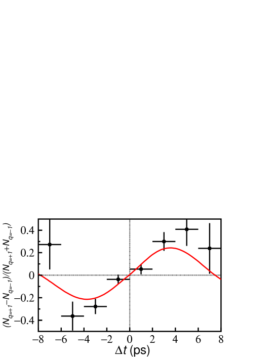
Figure 11: The time dependent asymmetry for $B^{0}$ and ${\bar{B}^{0}}$ decays to ${\bar{c}}cK_{S}^{0}$ ($\xi_{\rm CP}=-1$). The amplitude of this oscillation, extracted from an event-by-event maximum likelihood fit, gives $\sin 2\phi_{1}=0.716\pm 0.083$.

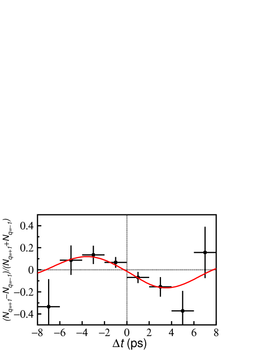
Figure 12: The time dependent asymmetry for $B^{0}$ and ${\bar{B}^{0}}$ decays to $J/\psi K_{L}^{0}$ ($\xi_{\rm CP}=1$). The amplitude of this oscillation, extracted from an event-by-event maximum likelihood fit, gives $\sin 2\phi_{1}=0.781\pm 0.167$.

We first perform this fit separately for candidates with $CP=-1$ (the bulk of our data) and $CP=+1$ (our $J/\psi K^{0}_{L}$ sample), shown in figs. 11 and 12, respectively. We find the magnitude of the fit asymmetries are equal, but they have opposite sign – as expected. The fit results are reported in table 3. We then combine all candidates into a single fit (see fig. 13) – inverting the sign of $\Delta t$ for the $CP=+1$ candidates – and obtain:

$$\sin 2\phi_{1}=0.719\pm 0.074(stat.)\pm 0.035(sys.)$$

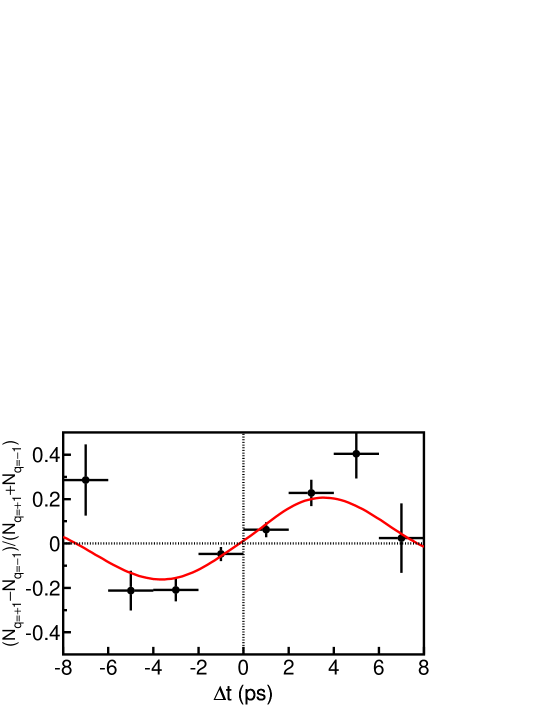
Figure 13: The combined time dependent asymmetry for $B^{0}$ and ${\bar{B}^{0}}$ decays to all ${\bar{c}}cK^{0}$ final states (flipping the sign of the candidates with $\xi_{\rm CP}=1$). An event-by-event maximum likelihood fit gives $\sin 2\phi_{1}=0.719\pm 0.074$.

The systematic uncertainties involved in this measurement are listed in table 2. The largest of these uncertainties are derived from measurements of our control samples – for example the flavour tagging discussed in section 3.2 – and thus can be expected to shrink as more data becomes available [5]. The overall systematic uncertainty is small compared to the statistical precision which bodes well for future measurements.

Uncertainty Source	Value
Vertexing Reconstruction	0.022
Flavour Tagging	0.015
Vertex Resolution	0.014
Fit parametrisation	0.011
$J/\psi K_{L}^{0}$ Background	0.010
$\Delta m_{d}$, $\tau_{B}$	$\leq 0.010$
Total	0.035

Table 2: Systematic uncertainties on the measurement of $\sin 2\phi_{1}$.

3.5 Cross-checks of $\sin 2\phi_{1}$

We perform a number of cross-checks on non-$CP$ eigenstate samples, all of which exhibit null asymmetries with statistical precisions ranging from $0.02$ to $0.09$. We do not include these as systematic uncertainties as we find no evidence of bias but they provide additional confidence in our main result. We have also sub-divided our data into different sub-samples to see whether there is any evidence for systematic variations in our result. Finding none (see table 3) gives us further confidence in our main result but again do not ascribe additional systematic uncertainty as the variations are all consistent with our quoted result within the statistics of the smaller sub-samples involved.

Subsample (stat error only)
$J/\psi K_{S}^{0}(\pi^{+}\pi^{-})$	$0.73\pm 0.10$
$(c{\bar{c}})K_{S}^{0}$ (except $J/\psi K_{S}^{0}(\pi^{+}\pi^{-})$)	$0.67\pm 0.17$
$J/\psi K^{0}_{L}$	$0.78\pm 0.17$
$f_{tag}=B^{0}$	$0.65\pm 0.12$
$f_{tag}={\bar{B}^{0}}$	$0.77\pm 0.09$
$r\leq 0.5$	$1.26\pm 0.36$
$0.5\leq r\leq 0.75$	$0.62\pm 0.15$
$0.75\leq r$	$0.72\pm 0.09$
All	$0.72\pm 0.07$

Table 3: Cross-checks of $\sin 2\phi_{1}$ from fits to subsets of the data.

4 $CP$ Asymmetries in $B^{0}\rightarrow\pi^{+}\pi^{-}$ Decay

Having observed indirect $CP$ violation in $B\rightarrow J/\psi K$ decays it is natural to study other $CP$ eigenstates. The decay $B^{0}\rightarrow\pi^{+}\pi^{-}$ is interesting because there are at least two significant amplitudes that can interfere in the direct decay. These amplitudes are show diagrammatically in fig. 14. With more than one amplitude in the direct decay path one can have a $\cos\Delta m\Delta t$ dependence in the $CP$ asymmetry. This dependence can come from the interference of the direct amplitudes and can appear in addition to the $\sin\Delta m\Delta t$ time-dependence (compare for example to eqn. 1) from the interference with the mixing amplitude:

$A_{CP}(\Delta t)$	=	${{{dN\over dt}(\bar{B^{0}}\rightarrow F_{\rm CP}})-{dN\over dt}(B^{0}\rightarrow F_{\rm CP})}\over{{dN\over dt}(\bar{B^{0}}\rightarrow F_{\rm CP})+{dN\over dt}(B^{0}\rightarrow F_{\rm CP})}$,
	=	$S_{F}\sin~{}\Delta m\Delta t+A_{F}\cos~{}\Delta m\Delta t.\qquad\qquad[2]$

The $B^{0}\rightarrow K^{+}\pi^{-}$ branching fraction – three times larger than the $B^{0}\rightarrow\pi^{+}\pi^{-}$ branching fraction – is strong evidence that the penguin amplitude (right diagram in fig. 14) is not small. In the decay $B^{0}\rightarrow\pi^{+}\pi^{-}$ the CKM elements involved predict an asymmetry proportional to the angle $\phi_{2}$. However the penguin diagram can introduce a non-CKM phase thus:

$$S_{F}\approx\sin(2\phi_{2}+\theta)$$

where $\theta$ can come from phases at the gluon vertices in the penguin process. While waiting for measurements of the various $B\rightarrow\pi\pi$ branching fractions [6] with sufficient precision to constrain $\theta$, it is still interesting to measure the $\pi^{+}\pi^{-}$ asymmetry and perhaps get some hint for the size of the combination $\sin(2\phi_{2}+\theta)$ [7].

Figure 14: Two tree level diagrams for $B^{0}\rightarrow\pi^{+}\pi^{-}$ decays. Given that there are two paths to the same $CP$ eigenstate, their interference can produce direct $CP$ violation in this mode.

4.1 $B^{0}\rightarrow\pi^{+}\pi^{-}$ Candidate Selection

The candidates and result presented here are from 43 fb^-1 of data collected by Belle [8]. While the $B$ vertexing and flavour tagging described in sections 3.1 and 3.2 can be used in a measurement of the $\pi^{+}\pi^{-}$ asymmetry, the candidate selection is more challenging. The branching fractions for $B\rightarrow h^{+}h^{-}$ are an order of magnitude smaller than those of the $c{\bar{c}}K$ final states – on the order of $10^{-5}$. Furthermore the $B\rightarrow h^{+}h^{-}$ decays have only two, relatively high momentum, tracks in the final state. Such candidates are much more prone to look like the $e^{+}e^{-}\rightarrow q{\bar{q}}$ continuum background. Belle uses a set of event-shape variables (Fox-Wolfram moments) and the reconstructed $B^{0}$ candidate direction to suppress continuum background. These are combined into a single variable, $R$, shown in figure 15 for $B{\bar{B}}$ data (open circles) and off-resonance data (closed circles). By requiring $R>0.8$ we reduce the continuum background by an order of magnitude while retaining two thirds of our $B$ candidates.

Figure 15: Low multiplicity final states are subject to higher background from the $e^{+}e^{-}$ continuum. To suppress these Belle combines event shape variables to get an overall likelihood, $R$. The solid points are continuum data, while the open points are a control sample of fully reconstructed, low-multiplicity, $B$ candidates. $B^{0}\rightarrow\pi^{+}\pi^{-}$ candidates are required to have $R>0.8$.

Since these events are fully reconstructed we are able to measure both the beam-constrained mass, m_bc, and the difference between the reconstructed energy of the $B$ candidate and the beam energy, $\Delta E$. Figure 16 shows the distributions of both of these variables for our $B\rightarrow h^{+}h^{-}$ sample. Comparing the m_bc distribution for these candidates to that of the $c{\bar{c}}K$ candidates in fig. 9 one sees that the background is much more prominent. In the $\Delta E$ distribution (on the right in fig. 16) one can see the source of these backgrounds. The remaining continuum background populates $\Delta E$ almost uniformly – falling linearly with increasing $\Delta E$ due to phase space – and is represented by the dotted line. $B$ decays to three or more particles, where we have missed one in our reconstruction, populate the low $\Delta E$ region (grey line) at a much lower rate than the continuum. Finally, $B^{0}\rightarrow K^{+}\pi^{-}$ candidates that have not been rejected by our particle identification produce a peak at $\Delta E\approx-0.045$ GeV. This peak is shifted because these candidates have been reconstructed assuming that both $B^{0}$ decay daughter tracks are pions (with a mass of 139 MeV/c²). If one of them is really a kaon (with a mass of 494 MeV/c²) then the reconstructed energy shifts down by about 45 MeV. This background is shown by the dot-dashed line.

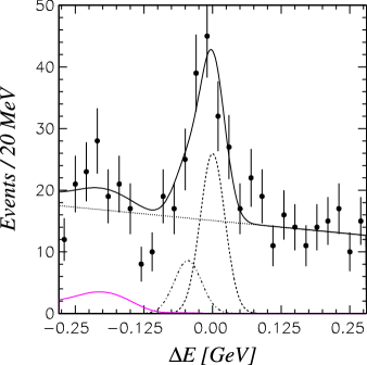
Figure 16: Left: The beam constrained mass, m_bc, for the $B^{0}\rightarrow\pi^{+}\pi^{-}$ candidates used to extract the $CP$ asymmetry. Right: The energy difference distribution, $\Delta E$, for the same candidates. In $\Delta E$ the $\pi^{+}\pi^{-}$ signal peaks at 0 (dashed Gaussian), the $K^{+}\pi^{-}$ background peaks at -0.045 GeV (dot-dashed Gaussian). The continuum is parametrised as a falling linear background (dotted line) while $B^{0}$ decays with more that two particles in the final state appear at low $\Delta E$.

We restrict our $CP$ fit to candidates that have $|\Delta E|<0.067$ GeV, eliminating the mis-reconstructed $B$ background entirely and leaving us with 74 $\pi^{+}\pi^{-}$ candidates, 28 $K^{+}\pi^{-}$ candidates and about 100 candidates that come from the $e^{+}e^{-}$ continuum.

4.2 The $CP$ Fit

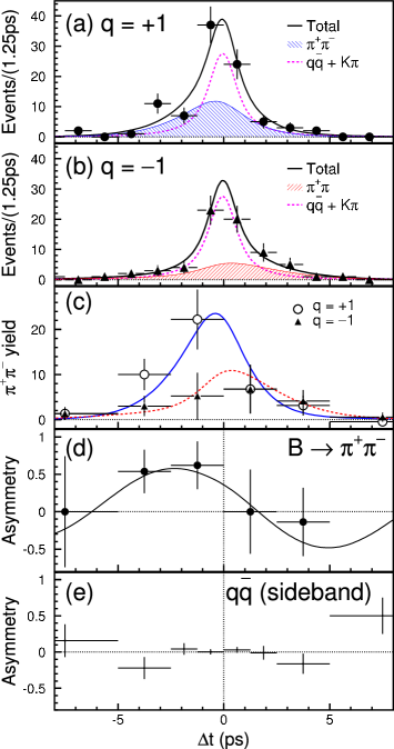
Figure 17: The results of the $\pi^{+}\pi^{-}\>\>CP$ asymmetry fit. a) The $\Delta t$ distribution for candidates tagged with $q=1$. The signal is shown as the hatched region, while the background (dominated by the continuum) is shown by the dashed line. The solid line is a projection of the overall fit and the points are the data. b) The $\Delta t$ distribution for candidates with tagged $q=-1$. c) The circles (triangles) are the background subtracted data for $q=(-)1$ while the curves are fit projections for the two flavours. d) The difference between the two data-samples in c). e) The asymmetry observed in a continuum sample.

We perform an event-by-event likelihood fit to the time dependent asymmetry for the $B\rightarrow\pi^{+}\pi^{-}$ candidates. In order to maximise our sensitivity to the $\pi^{+}\pi^{-}$ asymmetry this fit weights the events according to their continuum likelihood (events near $R=1$ are weighed more heavily) as well as their flavour tagging probability and vertex reconstruction quality – as was done for $\sin 2\phi_{1}$.

Figures 17 a) and b) show the $\Delta t$ distributions for events tagged as coming from $B^{0}$ and ${\bar{B}^{0}}$ decays, respectively. The continuum and $K^{+}\pi^{-}$ backgrounds are represented by the dashed lines, symmetric about $\Delta t=0$ in each case. The hatched areas in each plot are what the fit ascribes to the $B\rightarrow\pi^{+}\pi^{-}$ candidates. The sum of these two distributions give the solid line which fits the data. Figure 17 c) shows the $\Delta t$ distribution for just the $B\rightarrow\pi^{+}\pi^{-}$ component of the fit. Here we see that our fit predicts that there are almost twice as many $B^{0}$ as ${\bar{B}^{0}}$ candidates in our sample – independent of $\Delta t$ – an indication of direct $CP$ violation. Finally, fig. 17 d) shows the asymmetry between the two distributions in fig. 17 c). Here one also sees a $\Delta t$ dependent asymmetry leading to our fit result:

$S_{\pi\pi}$ =	$-$	$1.21^{+0.38}_{-0.27}({\rm stat})$	${}^{+0.16}_{-0.13}({\rm sys})$,
$A_{\pi\pi}$ =		$0.94^{+0.25}_{-0.31}({\rm stat})$	$\pm 0.09({\rm sys})$.

This is three sigma evidence for both direct $CP$ violation in the decay $B\rightarrow\pi^{+}\pi^{-}$ and indirect $CP$ violation [8].

We have performed a large number of cross-checks on this fit, including fits to the $B^{0}\rightarrow K^{+}\pi^{-}$ sample which should not have a $CP$ violating asymmetry and fits to continuum side-bands (fig. 17 e). None of these fits show significant asymmetries. We have simulated the size of our statistical uncertainties. We find that our statistical uncertainty on $S_{\pi\pi}$ is somewhat smaller than might be expected for a sample this size. Still there is a 5% chance that we could have gotten a smaller uncertainty. While unlikely, this is not an unacceptable statistical fluctuation. Finally, we have performed a series of toy Monte Carlo simulations, each generated with $(S_{\pi\pi},A_{\pi\pi})=(0,0)$ and sample sizes (signal and background) that mimic those in our data. We find that 1.6% of these toy Monte Carlo samples return a fit value farther from $(S_{\pi\pi},A_{\pi\pi})=(0,0)$ than our data. It will be interesting to see how this result evolves as more data becomes available.

5 $CP$ Asymmetries in Rarer $B^{0}$ Decay Modes

Having looked at two of the more plentiful $B$ meson decays that are $CP$ eigenstates, we turn to the next most likely $B$ decay modes to show $CP$ phases. One such class of decays is shown in fig. 18. With no tree level contribution these decay processes might be expected to have branching fractions smaller than those discussed above. In fact, the mode $B\rightarrow\eta^{\prime}K^{0}_{S}$ has a branching ratio that is somewhat larger than the mode $B\rightarrow\pi^{+}\pi^{-}$ and clearly larger than the, as yet unseen, decay $B\rightarrow\eta K$. That the $\eta^{\prime}K$ branching ratio is so large (about $5\times 10^{-5}$) is not easy to understand theoretically – hinting that there may be more that just a charged $W$ boson involved in the loop at the top of the diagram. If there were contributions from a charged Higgs to this amplitude, it could introduce an additional phase, interfering with the weak phase predicted by the CKM model. In the absence of such additional phases this decay would provide another way – albeit a much lower statistics way – to measure $\sin 2\phi_{1}$. Thus a comparison of the $CP$ asymmetry in the decay $\eta^{\prime}K^{0}_{S}$ to that seen in $c{\bar{c}}K_{S}^{0}$ could help unravel the mystery of the large branching of $B$ mesons into this mode and may provide a glimpse of physics beyond the Standard Model.

Figure 18: The Feynman-diagram for the decay $B^{0}\rightarrow\eta^{\prime}K^{0}_{S}$. The unexpectedly large branching fraction into this mode hints that there may be extra contributions to the amplitude – which could introduce additional $CP$ phases.

5.1 $CP$ Asymmetry in the Decay $B^{0}\rightarrow\eta^{\prime}K^{0}_{S}$

Figure 19 shows the beam constrained mass distribution for 128 candidate $B^{0}\rightarrow\eta^{\prime}K^{0}_{S}$ decays from 78 fb^-1 of Belle data. Here the $\eta^{\prime}$ candidates have been reconstructed in $\eta\>\pi^{+}\pi^{-}$ and $\rho^{0}\gamma$ intermediate states and then combined with $K_{S}^{0}\rightarrow\pi^{+}\pi^{-}$ combinations. The plot on the right of fig. 19 shows the $B^{0}{\bar{B}^{0}}$ asymmetry, as a function of $\Delta t$, where the candidates have been flavour tagged and vertexed in the same way as our $c{\bar{c}}K^{0}_{S}$ measurement of $\sin 2\phi_{1}$. The coefficient for indirect $CP$ violation derived from this fit (eqn. 4 with $A\equiv 1$) is listed in table 4. While the statistics are still poor, this is a demonstration that we can measure $CP$ asymmetries in these rare modes. More details on this analysis can be found in reference [9] that describes this measurement made on the first half of the data shown here.

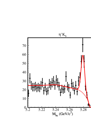
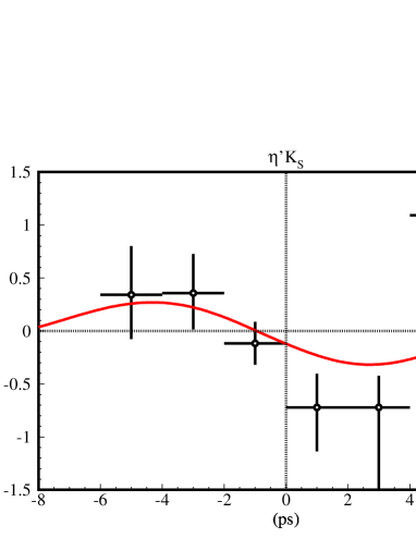
Figure 19: Left: The beam constrained mass distribution for $B^{0}\rightarrow\eta^{\prime}K^{0}_{S}$ candidates. Right: The $CP$ asymmetry as a function of $\Delta t$ for these candidates.

Mode	$(\sin 2\phi_{1})_{\rm eff}$	Candidates
$\eta^{\prime}K_{S}^{0}$	$0.76\pm 0.36({\rm stat})\pm 0.06({\rm sys})$	128
$\phi K_{S}^{0}$	$-0.73\pm 0.64({\rm stat})\pm 0.18({\rm sys})$	35
$(K^{+}K^{-})_{\rm non-res}K_{S}^{0}$	$0.52\pm 0.46({\rm stat})\pm 0.11({\rm sys})^{+0.27}_{-0.03}({\rm CP})$	95

Table 4: $CP$ fit parameters for $b\rightarrow s{\bar{s}}s$ decay modes.

We perform the same analysis on samples of $B^{0}\rightarrow K^{+}K^{-}K^{0}_{S}$ decays. Though the number of candidates in this sample is even smaller, we can begin to probe their $CP$ asymmetry. We separate the $K^{+}K^{-}$ candidates into two samples. When $m_{K^{+}K^{-}}\approx m_{\phi}$ the final state has $CP=-1$ providing another potentially clean determination of $\sin 2\phi_{1}$. The statistics limited result is shown in table 4. The remaining sample is somewhat larger, providing a more incisive measurement of the $CP$ asymmetry. Studies of similar non-resonant decays related to this one by isospin (such as $B^{+}\rightarrow K^{+}K^{0}{\bar{K}^{0}}$) have shown that our $(K^{+}K^{-})_{\rm non-res}K_{S}^{0}$ sample is $97^{+3}_{-16}\%$ $CP$ even. This bound on the $CP$ symmetry of the non-resonant $K^{+}K^{-}$ final state translates into an additional systematic on the effective $\sin 2\phi$, listed in table 4. The measurement of the $CP$ eigenvalue in this mode will improve with additional data so the non-resonant mode might eventually provide another clean measurement of $\sin 2\phi_{1}$, or a glimpse of a non-Standard Model phase this decay.

6 Summary and Future Prospects

Belle has studied the decay of $B^{0}$ mesons into a number of $CP$ eigenstates. The most precise measurement of $\sin 2\phi_{1}$ to date comes from the modes $B^{0}\rightarrow c{\bar{c}}K$. Most of the systematic uncertainties involved in that measurement come from calibrations of our flavour tagging and decay vertexing procedure based on control samples. Thus it is reasonable to expect that the precision on $\sin 2\phi_{1}$ – both statistical and systematic – will improve as more data becomes available. Figure 20 shows a prediction of how the precision on $\sin 2\phi_{1}$ will scale as Belle collects more data. The lowest curve shows the evolution of the systematic uncertainty on $\sin 2\phi_{1}$ in the $c{\bar{c}}K$ measurement. It should improve until as least 1000 fb^-1 (1 ab^-1) of data has been collected. At that point we expect an overall precision (uppermost thin line in fig. 20) of $\delta\sin 2\phi_{1}\approx 0.025$.

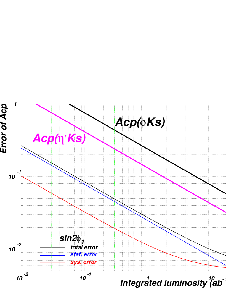
Figure 20: Prospects for improving the precision on $\sin 2\phi_{1}$ from the decay $c{\bar{c}}K^{0}_{S}$ (lower set of thin curves) with additional statistics. For comparison the precision expected on rarer modes ($\eta^{\prime}K_{S}^{0}$ thick grey curve and $\phi K^{0}_{S}$ thick black curve) are also shown.

The rarer modes will also benefit from the increase in statistics. Belle expects to be able to accumulate 1 ab^-1 of data in the next 3 or 4 years. At that point the precision on the $\eta^{\prime}K^{0}_{S}$ asymmetry should approach the precision that we currently have on the $c{\bar{c}}K$ asymmetry. If there are other modes contributing to the phase in $\eta^{\prime}K^{0}_{S}$ decay un-natural fine-tuning would be necessary for our precision not to reveal some discrepancy between what would otherwise be two measurements of the same quantity.

The $B$ factories were built to confirm the $CP$ violation predicted by the CKM model in $B^{0}$ meson decay – they have now achieved that milestone. Having made a measurement of $\sin 2\phi_{1}$ with a precision of 10% in the $c{\bar{c}}K^{0}_{S}$ modes, and are now pushing to improve the precision to a few percent. At the same time they are expanding the scope of their study to other decay processes. In doing so they will measure other angles of the unitarity triangle. This will over-constrain the CKM model and test whether there is physics beyond the three known families of quarks and their Standard Model electroweak decays. In the coming years the flavour sector will become ever more constrained reducing the range of physics that could explain why we have three families of quarks.

References

- [1] M. Kobyashi and T. Maskawa, Prog. Theor. Phys. 49, 652 (1973).
- [2] A.B. Carter and A.I. Sanda, Phys. Rev. Lett. 45, 952, (1980).
- [3] K. Abe et al. (The Belle Collaboration), Observation of Mixing-induced CP Violation in the Neutral Meson System, Phys. Rev. D 66, 032007 (2002).
- [4] K. Abe et al. (The Belle Collaboration), Precise Measurement of Meson Lifetimes with Hadronic Decay Final States, Phys. Rev. Lett. 88, 171801 (2002).
- [5] K. Abe et al. (The Belle Collaboration), Improved Measurement of Mixing-induced CP Violation in the Neutral B Meson System, Phys. Rev. D 66, 071102(R), (2002).
- [6] B. Casey, these proceedings.
- [7] M. Gronau and J.L. Rosner, Strong and Weak Phases from Time-Dependent Measurements of , Phys. Rev. D 65, 093012 (2002).
- [8] K. Abe et al. (The Belle Collaboration), Study of CP-Violating Asymmetries in Decays, Phys. Rev. Lett. 89, 071801 (2002).
- [9] K.F. Chen, K. Hara et al. (The Belle Collaboration), Measurement of CP-Violating Parameters in Decays, Phys. Lett. B 546, 196 (2002).