Study of the Cabibbo-suppressed decay modes $D^{0}\rightarrow\pi^{-}\pi^{+}$ and $D^{0}\rightarrow K^{-}K^{+}$

Abstract

Using data from the FOCUS (E831) experiment at Fermilab, we present a new measurement for the branching ratios of the Cabibbo-suppressed decay modes $D^{0}\rightarrow\pi^{-}\pi^{+}$ and $D^{0}\rightarrow K^{-}K^{+}$. We measured:

$\Gamma(D^{0}\rightarrow K^{-}K^{+})/\Gamma(D^{0}\rightarrow\pi^{-}\pi^{+})=2.81\pm 0.10\textrm{(stat)}\pm 0.06\textrm{(syst)}$,

$\Gamma(D^{0}\rightarrow K^{-}K^{+})/\Gamma(D^{0}\rightarrow K^{-}\pi^{+})=0.0993\pm 0.0014\textrm{(stat)}\pm 0.0014\textrm{(syst)}$, and

$\Gamma(D^{0}\rightarrow\pi^{-}\pi^{+})/\Gamma(D^{0}\rightarrow K^{-}\pi^{+})=0.0353\pm 0.0012\textrm{(stat)}\pm 0.0006\textrm{(syst)}$.

These values have been combined with other experimental data to extract the ratios of isospin amplitudes and the phase shifts for the $D\rightarrow KK$ and $D\rightarrow\pi\pi$ decay channels.

$\textrm{The~{}FOCUS~{}Collaboration}^{\star}$ , , , , , , , , , , , , , , , , , , , , , , , , , , , , , , , , , , , , , , , , , , , , , , , , , , , , , , , , , , , , , , , , , , , , , , , , , , , , , , , , , , , , , , , , , , , , , , , , , , , , , , , , ,

1. Introduction

In recent years, hadronic decays of charm mesons in many decay modes have been extensively studied. The theoretical models that have been developed mainly describe the 2-body decay modes and these models have led to several successful predictions. However the branching ratio ${\frac{{\Gamma(D^{0}\rightarrow K^{-}K^{+})}}{{\Gamma(D^{0}\rightarrow\pi^{-}\pi^{+})}}}$ has, for a long time, been a puzzle of charm physics. The decay modes $D^{0}\rightarrow K^{-}K^{+}$ and $D^{0}\rightarrow\pi^{-}\pi^{+}$ are both Cabibbo-suppressed and in first order perturbative calculation both receive contributions from the same diagrams (external spectator and exchange). To first order in the SU(3) flavour symmetry limit, the above branching ratio should be one. However this ratio is reduced by a factor $0.86$ due to a phase space difference and increased by a factor of $(f_{K}/f_{\pi})^{2}=1.49$ because of the different decay constants of the kaon and the pion. An overall ratio of $1.29$ is thus expected. Including SU(3) breaking effects, the expected ratio can increase to an upper limit of about 1.4 [1, 2].

However, the measured ratio is close to $2.5$ [3]. Both penguin diagrams and final state interactions (FSI) have been proposed as sources of such a high value. However the penguin interference [4] seems to be unable to explain this large value. Some theoretical models [5, 6] propose the FSI as the solution of this puzzle.

In this paper we present a new measurement of the ${\frac{{\Gamma(D^{0}\rightarrow K^{-}K^{+})}}{{\Gamma(D^{0}\rightarrow\pi^{-}\pi^{+})}}}$ branching ratio obtained using data from the FOCUS experiment as well as an isospin analysis of the $D\rightarrow KK$ and $D\rightarrow\pi\pi$ decay channels.

FOCUS is a charm photoproduction experiment [7] which collected data during the 1996–97 fixed target run at Fermilab. Electron and positron beams (with typically $300~{}\textrm{GeV}$ endpoint energy) obtained from the $800~{}\textrm{GeV}$ Tevatron proton beam produce, by means of bremsstrahlung, a photon beam which interacts with a segmented BeO target. The mean photon energy for triggered events is $\sim 180~{}\textrm{GeV}$. A system of three multicell threshold Čerenkov counters performs the charged particle identification, separating kaons from pions up to $60~{}\textrm{GeV}/c$ of momentum. Two systems of silicon microvertex detectors are used to track particles: the first system consists of 4 planes of microstrips interleaved with the experimental target [8] and the second system consists of 12 planes of microstrips located downstream of the target. These detectors provide high resolution in the transverse plane (approximately $9~{}\mu\textrm{m}$), allowing the identification and separation of charm primary (production) and secondary (decay) vertices. The charged particle momentum is determined by measuring their deflections in two magnets of opposite polarity through five stations of multiwire proportional chambers.

2. Analysis of $D^{0}\rightarrow\pi^{-}\pi^{+}$ and $D^{0}\rightarrow K^{-}K^{+}$

The final states are selected using a candidate driven vertex algorithm [7]. A secondary vertex is formed from the two candidate tracks. The momentum of the resultant $D^{0}$ candidate is used as a seed track to intersect the other reconstructed tracks and to search for a primary vertex. The confidence levels of both vertices are required to be greater than $1\%$. Two estimators of the relative isolation of these vertices are returned by the algorithm: the first estimator (Iso1) being the confidence level that tracks forming the secondary vertex might come from the primary vertex, while the second estimator (Iso2) is the confidence level that other tracks in the event might be associated with the secondary vertex. Once the production and decay vertices are determined, the distance $L$ between them and its error $\sigma_{L}$ are computed. The quantity $L$ / $\sigma_{L}$ is an unbiased measure of the significance of detachment between the primary and secondary vertices. These variables provide a good measure of the topological configuration of the event, so that appropriate cuts on them reject the combinatorial background effectively.

In addition to large combinatorial backgrounds, $D^{0}\rightarrow\pi^{-}\pi^{+}$ and $D^{0}\rightarrow K^{-}K^{+}$ decays are difficult to isolate because of a large reflection from the Cabibbo favored $D^{0}\rightarrow K^{-}\pi^{+}$ decays. Particle identification requirements for each decay mode have been chosen to optimize signal quality. To minimize systematic errors on the measurements of the branching ratios, we use identical vertex cuts on the signal and normalizing modes. The only difference in the selection criteria among different decay modes lies in the particle identification cuts.

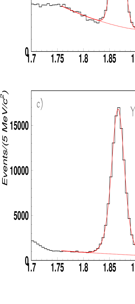
Figure 1: Invariant mass distribution for $\pi^{-}\pi^{+}$(a), $K^{-}K^{+}$(b) and $K^{-}\pi^{+}$(c). The fit (solid curve) for the Cabibbo-suppressed decay modes of $D^{0}$ is to a gaussian over a polynomial (for the combinatorial background) and a function obtained with Monte Carlo simulations for the reflection peak.

In the $D^{0}\rightarrow\pi^{-}\pi^{+}$ and $D^{0}\rightarrow K^{-}K^{+}$ analysis, we require $L$ / $\sigma_{L}$ $>$ $10$, Iso1 $<10\%$ and Iso2 $<$ 0.5 $\%$. We also require the $D^{0}$ momentum to be in the range $25\rightarrow 250~{}\textrm{GeV}/c$ (a very loose cut) and the primary vertex to be formed with at least two reconstructed tracks in addition to the seed track. The Čerenkov identification cuts used in FOCUS are based on likelihood ratios between the various stable particle identification hypotheses. These likelihoods are computed for a given track from the observed firing response (on or off) of all the cells that are within the track’s ($\beta=1$) Čerenkov cone for each of our three Čerenkov counters. The product of all firing probabilities for all the cells within the three Čerenkov cones produces a $\chi^{2}$-like variable $W_{i}=-2\ln(\mathrm{Likelihood})$ where $i$ ranges over the electron, pion, kaon and proton hypotheses [9]. All the kaon tracks are required to have $\Delta_{K}=W_{\pi}-W_{K}$ (kaonicity) greater than $1$, whereas all the pion tracks are required to have $\Delta_{\pi}=W_{K}-W_{\pi}$ (pionicity) exceeding $1.5$. Using the set of selection cuts just described, we obtain the invariant mass distributions for $\pi^{-}\pi^{+}$, $K^{-}K^{+}$ and $K^{-}\pi^{+}$ shown in Fig. 1.

In Fig. 1a the $\pi^{-}\pi^{+}$ mass plot shows a broad peak to the left of the signal peak due to surviving contamination from $D^{0}\rightarrow K^{-}\pi^{+}$ events. The shape of the reflection peak has been determined by generating Monte Carlo $D^{0}\rightarrow K^{-}\pi^{+}$ events and reconstructing them as $\pi^{-}\pi^{+}$. The mass plot is fit with a function that includes a Gaussian for the signal, a third-order polynomial for the combinatorial background and a shape for the reflection background obtained from the Monte Carlo simulation. The amplitude of the reflection peak is a fit parameter while its shape was fixed. The low mass region is excluded in the fit to avoid possible contamination due to other charm hadronic decays involving an additional $\pi^{0}$. A least squares fit gives a signal of $3453\pm 111$$\pi^{-}\pi^{+}$ events.

The $K^{-}K^{+}$ mass plot, shown in Fig. 1b, is fit with a function similar to that for the $\pi^{-}\pi^{+}$ fit. In the $K^{-}K^{+}$ case, the reflection peak is on the right of the signal. The fit gives a signal of $10830\pm 148$$K^{-}K^{+}$ events.

The large statistics $K^{-}\pi^{+}$ mass plot of Fig. 1c is fit with two Gaussians with the same mean but different sigmas to take into account the different resolution in momentum of our spectrometer [7] plus a second-order polynomial. The fit gives a signal of $105030\pm 372$$K^{-}\pi^{+}$ events.

The fitted $D^{0}$ masses are in good agreement with the world average [3] and the widths are in good agreement with those of our Monte Carlo simulation.

3. Relative Branching Ratios

The evaluation of relative branching ratios requires yields from the fits to be corrected for detection efficiencies, which differ among the various decay modes because of differences in both spectrometer acceptance (due to different $Q$ values for the various decay modes) and Čerenkov identification efficiency.

From the Monte Carlo simulations, we compute the relative efficiencies to be: ${\frac{\epsilon(D^{0}\rightarrow\pi\pi)}{\epsilon(D^{0}\rightarrow KK)}}=0.897\pm 0.003$, ${\frac{\epsilon(D^{0}\rightarrow K\pi)}{\epsilon(D^{0}\rightarrow KK)}}=0.963\pm 0.003$ and ${\frac{\epsilon(D^{0}\rightarrow K\pi)}{\epsilon(D^{0}\rightarrow\pi\pi)}}=1.074\pm 0.004$. Using the previous results, we obtain the following values for the branching ratios: ${\frac{{\Gamma(D^{0}\rightarrow KK)}}{{\Gamma(D^{0}\rightarrow\pi\pi)}}}=2.81\pm 0.10$, ${\frac{{\Gamma(D^{0}\rightarrow KK)}}{{\Gamma(D^{0}\rightarrow K\pi)}}}=0.0993\pm 0.0014$, and ${\frac{{\Gamma(D^{0}\rightarrow\pi\pi)}}{{\Gamma(D^{0}\rightarrow K\pi)}}}=0.0353\pm 0.0012$.

Systematic uncertainties on branching ratio measurements can come from different sources. We determine three independent contributions to the systematic uncertainty: the split sample component, the fit variant component, and the limited statistics of the Monte Carlo.

The split sample component takes into account the systematics introduced by a residual difference between data and Monte Carlo, due to a possible mismatch in the reproduction of the $D^{0}$ momentum and the changing experimental conditions of the spectrometer during data collection. This component has been determined by splitting data into four independent subsamples, according to the $D^{0}$ momentum range (high and low momentum) and the configuration of the vertex detector, that is, before and after the insertion of an upstream silicon system. A technique, employed in FOCUS and in the predecessor experiment E687, modeled after the S-factor method from the Particle Data Group [3], was used to try to separate true systematic variations from statistical fluctuations. The branching ratio is evaluated for each of the $4~{}(=2^{2})$ statistically independent subsamples and a scaled variance $\tilde{\sigma}$ (that is, where the errors are boosted when $\chi^{2}/(N-1)>1$) is calculated. The split sample variance $\sigma_{\textrm{split}}$ is defined as the difference between the reported statistical variance and the scaled variance, if the scaled variance exceeds the statistical variance:

$$\sigma_{\textrm{split}} =\sqrt{\tilde{\sigma}^{2}-\sigma_{\textrm{stat}}^{2}}\hskip 28.45274pt if\quad\tilde{\sigma}>\sigma_{\textrm{stat}}$$ (1)

$$\sigma_{\textrm{split}} =0\hskip 68.28644pt\quad if\quad\tilde{\sigma}<\sigma_{\textrm{stat}}\quad.$$

Another possible source of systematic uncertainty is the fit variant. This component is computed by varying, in a resonable manner, the fitting conditions on the whole data set. In our study, we changed the background parametrization (varying the degree of the polynomial), the fit function for the reflection peak (the reflection shape from the Monte Carlo was replaced by a Gaussian), and the use of two Gaussian for the fit of the peak of $D^{0}\rightarrow\pi^{-}\pi^{+}$ and $D^{0}\rightarrow K^{-}K^{+}$. The values obtained by the various fits are all a priori likely, therefore this uncertainty can be estimated by the simple average of the measures of the fit variants:

$$\sigma_{\textrm{fit}}=\sqrt{\frac{\sum_{i=1}^{N}x_{i}^{2}-N\langle x\rangle^{2}}{N-1}}\quad.$$ (2)

Finally, there is a further contribution due to the limited statistics of the Monte Carlo simulation used to determine the efficiencies. Adding in quadrature the three components, we get the final systematic errors summarized in Table 1:

Source	$\sigma_{\textrm{BR}(KK/K\pi)}$	$\sigma_{\textrm{BR}(\pi\pi/K\pi)}$
Split sample	$0.0005$	$0.0000$
Fit variant	$0.0012$	$0.0006$
MC statistics	$0.0003$	$0.0001$
Total systematic	$0.0014$	$0.0006$

Table 1: Sources of uncertainty on the $\frac{\Gamma(K^{-}K^{+})}{\Gamma(K^{-}\pi^{+})}$ and $\frac{\Gamma(\pi^{-}\pi^{+})}{\Gamma(K^{-}\pi^{+})}$ branching ratios.

The final results are shown in Table 2 along with a comparison with the previous determinations.

Experiment	$\frac{\Gamma(D^{0}\rightarrow K^{-}K^{+})}{\Gamma(D^{0}\rightarrow K^{-}\pi^{+})}$	$\frac{\Gamma(D^{0}\rightarrow\pi^{-}\pi^{+})}{\Gamma(D^{0}\rightarrow K^{-}\pi^{+})}$	$\frac{\Gamma(D^{0}\rightarrow K^{-}K^{+})}{\Gamma(D^{0}\rightarrow\pi^{-}\pi^{+})}$
E687 [10]	$0.109\pm 0.007\pm 0.009$	$0.043\pm 0.007\pm 0.003$	$2.53\pm 0.46\pm 0.19$
E791 [11]	$0.109\pm 0.003\pm 0.003$	$0.040\pm 0.002\pm 0.003$	$2.75\pm 0.15\pm 0.16$
CLEO [12]	$0.1040\pm 0.0033\pm 0.0027$	$0.0351\pm 0.0016\pm 0.0017$	$2.96\pm 0.16\pm 0.15$
E831 (this result)	$0.0993\pm 0.0014\pm 0.0014$	$0.0353\pm 0.0012\pm 0.0006$	$2.81\pm 0.10\pm 0.06$

Table 2: Comparison with other experiments.

4. Isospin analysis of $D\rightarrow KK$ and $D\rightarrow\pi\pi$ channels

Final State Interactions (FSI) can dramatically modify the observed decay rates and complicate the comparison of the experimental data with the theoretical predictions. By means of the isospin analysis of the decay channels $D\rightarrow KK$ and $D\rightarrow\pi\pi$, we can gain some insight on the elastic component of the FSI (pure rotation in isospin space).

Let us consider the $D\rightarrow\pi\pi$ transistions: $D^{0}\rightarrow\pi^{-}\pi^{+}$, $D^{0}\rightarrow\pi^{0}\pi^{0}$ and $D^{+}\rightarrow\pi^{+}\pi^{0}$. The decay amplitudes can be expressed in terms of isospin $I_{f}=0~{}(A_{0})$ and $I_{f}=2~{}(A_{2})$ amplitudes. The final state with isospin $I_{f}=1$ is forbidden by Bose statistics for an angular momentum zero system of two pions. We denote by $A^{+-}$, $A^{00}$ and $A^{+0}$ the decay amplitudes for the $D^{0}\rightarrow\pi^{-}\pi^{+}$, $D^{0}\rightarrow\pi^{0}\pi^{0}$ and $D^{+}\rightarrow\pi^{+}\pi^{0}$, respectively. Expressing the decay amplitude in terms of isospin amplitudes, we have [13, 14, 15]:

$$A^{+-} = +\sqrt{\frac{2}{3}}|A_{0}|\exp{(i\delta_{0})}+\sqrt{\frac{1}{3}}|A_{2}|\exp{(i\delta_{2})}$$ (3)

$$A^{00} = -\sqrt{\frac{1}{3}}|A_{0}|\exp{(i\delta_{0})}+\sqrt{\frac{2}{3}}|A_{2}|\exp{(i\delta_{2})}$$ (4)

$$A^{+0} = +\sqrt{\frac{3}{2}}|A_{2}|\exp{(i\delta_{2})}\quad.$$ (5)

Adding the decay amplitudes in quadrature, we find the ratio of the magnitude of isospin amplitudes and their relative phase shift difference in terms of measured branching fractions:

$$\mid\frac{A_{2}}{A_{0}}\mid^{2} = \frac{\frac{2}{3}\mid A^{0+}\mid^{2}}{\mid A^{+-}\mid^{2}+\mid A^{00}\mid^{2}-\frac{2}{3}\mid A^{+0}\mid^{2}}$$ (6)

$$\cos(\delta_{2}-\delta_{0}) = \frac{3\mid A^{+-}\mid^{2}-6\mid A^{00}\mid^{2}+2\mid A^{+0}\mid^{2}}{4\sqrt{2\mid A^{+0}\mid^{2}}\sqrt{\frac{3}{2}(\mid A^{00}\mid^{2}+\mid A^{+-}\mid^{2})-\mid A^{+0}\mid^{2}}}\quad.$$ (7)

The decay rate $\Gamma(D^{0}\rightarrow\pi^{-}\pi^{+})$ has been determined from our measurement of the branching ratio $\frac{\Gamma(\pi^{-}\pi^{+})}{\Gamma(K^{-}\pi^{+})}$, whereas the other $D\rightarrow\pi\pi$ decay rates and lifetimes have been taken from the Particle Data Group compilation [3].

The results are shown in Table 3. In contrast to $K\rightarrow\pi\pi$ decays, where the transitions are dominated by the $I=1/2$ amplitude ($\Delta~{}I=1/2$ rule), the $A_{2}$ amplitude in $D\rightarrow\pi\pi$ is comparable to the $A_{0}$ amplitude. Furthermore, there is a large phase shift difference between the isospin amplitudes. According to Watson’s theorem [16], this phase shift cannnot arise from the weak processes alone and thus constitutes direct evidence for FSI [17].

In the same way, we can consider the two-body $D\rightarrow KK$ transitions: $D^{0}\rightarrow K^{+}K^{-}$, $D^{0}\rightarrow K^{0}\mbox{\={K}}^{0}$ and $D^{+}\rightarrow K^{+}\mbox{\={K}}^{0}$. The decay amplitudes $A^{ij}$ for the $D\rightarrow K^{i}K^{j}$ decay modes can be expressed in terms of $A_{0}$ and $A_{1}$ isospin amplitudes [18]:

$$A^{+-} = \frac{1}{\sqrt{2}}\left(|A_{1}|\exp{(i\delta_{1})}+|A_{0}|\exp{(i\delta_{0})}\right)$$ (8)

$$A^{00} = \frac{1}{\sqrt{2}}\left(|A_{1}|\exp{(i\delta_{1})}-|A_{0}|\exp{(i\delta_{0})}\right)$$ (9)

$$A^{+0} = \sqrt{2}|A_{1}|\exp{(i\delta_{1})}\quad.$$ (10)

Using the previous decompositions, we can express the ratio of the magnitudes of the isospin amplitudes and their phase shift difference in terms of the measured branching fractions:

$$\mid\frac{A_{1}}{A_{0}}\mid^{2} = \frac{\mid A^{0+}\mid^{2}}{2\mid A^{+-}\mid^{2}+2\mid A^{00}\mid^{2}-\mid A^{+0}\mid^{2}}$$ (11)

$$\cos(\delta_{1}-\delta_{0}) = \frac{\mid A^{+-}\mid^{2}-\mid A^{00}\mid^{2}}{\sqrt{\mid A^{+0}\mid^{2}}\sqrt{2\mid A^{00}\mid^{2}+2\mid A^{+-}\mid^{2}-\mid A^{+0}\mid^{2}}}\quad.$$ (12)

The $\Gamma(D^{0}\rightarrow K^{-}K^{+})$ decay rate has been determined from our measurement of the branching ratio $\frac{\Gamma(K^{-}K^{+})}{\Gamma(K^{-}\pi^{+})}$, the $\Gamma(D^{+}\rightarrow K^{+}\mbox{\={K}}^{0})$ from a previous measurement of FOCUS [19] and the remaining decay rate from the Particle Data Group compilation [3].

The results are shown in Table 3. Analogously to the $D\rightarrow\pi\pi$ case, the two $D\rightarrow KK$ isospin amplitudes are of the same order of magnitude, although the isospin phase shift difference is smaller.

The isospin analysis of the $D\rightarrow KK$ and $D\rightarrow\pi\pi$ decay channels is summarized in Table 3 (the quoted errors are obtained adding in quadrature the statistical and systematic errors) along with a comparison to previous determinations by CLEO [15, 18]:

Quantity	CLEO	E831(this result)
$\mid A_{2}\mid/\mid A_{0}\mid$	$0.72\pm 0.13\pm 0.11$	$0.65\pm 0.14$
$\delta_{2}-\delta_{0}$	$(82.0\pm 7.5\pm 5.2)^{\circ}$	$(83.6\pm 10.0)^{\circ}$
$\mid A_{1}\mid/\mid A_{0}\mid$	$0.61^{+0.11}_{-0.10}$	$0.56\pm 0.04$
$\delta_{1}-\delta_{0}$	$(28.4^{+12.1}_{-9.7})^{\circ}$	$(37.1\pm 7.5)^{\circ}$

Table 3: Isospin analysis for $D\rightarrow KK$ and $D\rightarrow\pi\pi$ decay modes, where $\mid A_{2}\mid/\mid A_{0}\mid$ and $\delta_{2}-\delta_{0}$ refer to $D\rightarrow\pi\pi$, while $\mid A_{1}\mid/\mid A_{0}\mid$ and $\delta_{1}-\delta_{0}$ to $D\rightarrow KK$.

These results show that strong interactions, acting on the final particles, play a very important role in $D\rightarrow KK$ and $D\rightarrow\pi\pi$ decays, modifying the measured $\frac{\Gamma(K^{-}K^{+})}{\Gamma(\pi^{-}\pi^{+})}$ ratio.

Another way to see the elastic FSI effect on the $\frac{\Gamma(K^{-}K^{+})}{\Gamma(\pi^{-}\pi^{+})}$ branching ratio is to compute the ratio of the sums over the $D^{0}$ isospin rotated decay modes [20]: $\frac{\Gamma(K^{-}K^{+})+\Gamma(K^{0}\bar{K}^{0})}{\Gamma(\pi^{-}\pi^{+})+\Gamma(\pi^{0}\pi^{0})}$. As opposed to the $\frac{\Gamma(K^{-}K^{+})}{\Gamma(\pi^{-}\pi^{+})}$ ratio, this ratio is not affected by elastic FSI.

Using these measurements for $\frac{\Gamma(K^{-}K^{+})}{\Gamma(K^{-}\pi^{+})}$ and $\frac{\Gamma(\pi^{-}\pi^{+})}{\Gamma(K^{-}\pi^{+})}$ and the PDG [3] values for the other modes, we compute:

$$\frac{\Gamma(K^{-}K^{+})+\Gamma(K^{0}\bar{K}^{0})}{\Gamma(\pi^{-}\pi^{+})+\Gamma(\pi^{0}\pi^{0})}=2.06\pm 0.24\quad.$$ (13)

This ratio is lower than the $\frac{\Gamma(K^{-}K^{+})}{\Gamma(\pi^{-}\pi^{+})}$ branching ratio, but still above the expected value of $1.4$. Therefore, the elastic FSI cannot account for all the discrepancy between theory and experiments. An inelastic FSI that also allows the transition $KK\rightarrow\pi\pi$ seems to be the most reasonable explanation [5].

4. Conclusions

We have measured the following branching ratios: $\frac{\Gamma(D^{0}\rightarrow K^{-}K^{+})}{\Gamma(D^{0}\rightarrow K^{-}\pi^{+})}$, $\frac{\Gamma(D^{0}\rightarrow\pi^{-}\pi^{+})}{\Gamma(D^{0}\rightarrow K^{-}\pi^{+})}$ and $\frac{\Gamma(D^{0}\rightarrow K^{-}K^{+})}{\Gamma(D^{0}\rightarrow\pi^{-}\pi^{+})}$. A comparison with previous determinations has been shown in Table 2. Our results improve significantly the accuracy of these measurements.

An isospin analysis of the decay channels $D\rightarrow KK$ and $D\rightarrow\pi\pi$ shows that final state interactions play an important role in these hadronic decay modes.

We wish to acknowledge the assistance of the staffs of Fermi National Accelerator Laboratory, the INFN of Italy, and the physics departments of the collaborating institutions. This research was supported in part by the U. S. National Science Foundation, the U. S. Department of Energy, the Italian Istituto Nazionale di Fisica Nucleare and Ministero della Istruzione Università e Ricerca, the Brazilian Conselho Nacional de Desenvolvimento Científico e Tecnológico, CONACyT-México, and the Korea Research Foundation of the Korean Ministry of Education.

References

[1] A.J. Buras, J.M. Gerard and R. Ruckl, Nucl. Phys. B268 (1986)
16.
[2] M. Bauer, B. Steck and M. Wirbel, Z. Phys. C34 (1987) 103.
[3] K. Hagiwara et al. (Particle Data Group), Phys. Rev. D66 (2002) 010001.
[4] A.N. Kamal and T.N. Pham, Phys. Rev. D50 (1994) 1832.
[5] A.N. Kamal and R.C. Verma, Phys. Rev. D35 (1987) 3515;
A.N. Kamal and R. Sinha, Phys. Rev. D36 (1987) 3510;
A. Czarnecki, A.N. Kamal and Qi-ping Xu, Z. Phys. C54 (1992) 411.
[6] L.L. Chau and H.Y. Cheng, Phys. Lett. B280 (1992) 281.
[13] M. Gronau and D. London, Phys. Rev. Lett. 65 (1990)
3381.
[14] H.J. Lipkin, Y. Nir, H.R. Quinn and A.E. Snyder,
Phys. Rev. D44 (1991) 1454.
[15] CLEO collaboration, M. Selen et al.,
Phys. Rev. Lett. 71 (1993) 1973.
[16] K.M. Watson, Phys. Rev. 88 (1952) 1163;
J.F. Donoghue, E. Golowich, and B.R. Holstein, Dynamics of the
Standard Model, Cambridge University Press, 1992, page 510.
[17] J. Wiss, in Proceedings of the International School of
Physics Enrico Fermi, Varenna, Italy, 1997, IOS Press, Amsterdam,
1998, page 39.
[18] CLEO collaboration, M. Bishai et al.,
Phys. Rev. Lett. 78 (1997) 3261.
[19] FOCUS Collaboration, J.M. Link et al.,
Phys. Rev. Lett. 88 (2002) 041602.
[20] T.E. Browder, K. Honscheid and D. Pedrini, Annu. Rev.
Nucl. Part. Sci. 46 (1996) 395.