24.11.2002

Higgs Statistics for Pedestrians

Eilam Gross and Amit Klier

Department of Particle Physics

Weizmann Institute of Science, Rehovot 76100, Israel

email: eilam.gross@weizmann.ac.il

We review the results of the Standard Model Higgs boson search at LEP. An emphasis is put on revealing the details behind the statistical procedure developed by the LEP Higgs working group. The procedure is explained using a toy model which allows the reader to estimate the significance of the experimental observation which led at the time to a scientific debate on whether LEP has observed a 115 GeV Higgs boson.

1 Introduction

On 3 November 2000 in a seminar at CERN the LEP Higgs working group presented preliminary results of an analysis indicating a possible 2.9$\sigma$ observation of a 115 GeV Higgs boson [1]. Based on this analysis the four LEP collaborations requested the continuation of LEP to collect more data at $\sqrt{s}=208$ GeV. However, the arguments presented by the LEP collaborations did not convince the LEP management and in retrospect, it turned out that the LEP accelerator turn-off date of 2 November 2000 ended its eleven years of forefront research.

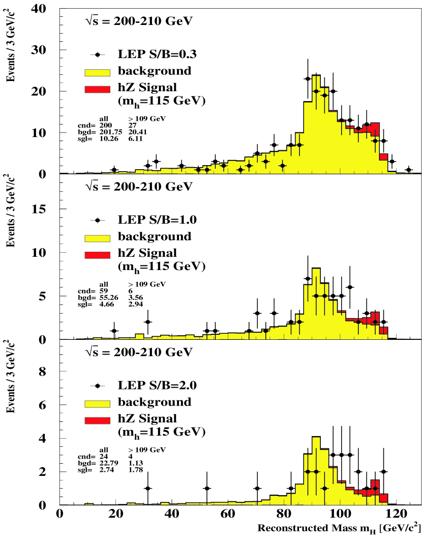
Figure 1: Distributions of the reconstructed Higgs mass, $m_{rec}$, obtained from three special, non-biasing, selections with increasing signal purity. In the loose/medium/tight selections the cuts are adjusted in such a way as to obtain, for a Higgs boson of 115 GeV mass, approximately 0.5/1/2 times as many expected signal as background events in the region $m_{rec}>109$ GeV[1].

Figure 1, taken from the above mentioned presentation, shows the reconstructed mass distribution of the background and the signal (on top of the background) with the data represented by the dots with error bars. It is shown for three possible selections of the data samples with increasing signal purity. None of these distributions shows a clear classical 3$\sigma$ excess of data over the expected background and some physicists claimed that this evidence was not convincing enough. However, the statistical arguments presented by the LEP Higgs working group were not based on these distributions, but rather on a sophisticated, though beautiful statistical analysis of the data. Two years after the event, when the last analysis of the LEP data indicated that the significance of a Higgs observation in the vicinity of 115 GeV went down to less than 2$\sigma$ [2], it becomes apparent that the LEP Standard Model (SM) Higgs heritage will in fact be a lower bound on the mass of the Higgs boson. However, the LEP Higgs working group has taught us powerful and instructive lessons of statistical methods for deriving limits and confidence levels in the presence of mass dependent backgrounds from various channels and experiments. These lessons will remain with us long after the lower bound becomes outdated.

In this note we are trying to repeat, in a pedagogical way, this LEP Higgs statistical lesson. To achieve this we developed a toy Monte Carlo model containing a simulated background and signal similar to LEP conditions at $\sqrt{s}=206$ GeV.

Due to mass resolution effects an event with a reconstructed mass $m_{rec}$ can originate from any Higgs mass in its vicinity. To appreciate the significance of a Higgs candidate with respect to some test mass $m_{H}$ the event weights are introduced in section 2.

The weights of all candidate events are summed up in section 3 to give the likelihood of an experiment in order to quantify its signal-like nature.

The probability density function of the likelihood is used in section 4 to estimate the probability of an experiment without a Higgs boson to fluctuate and give a more signal-like outcome than the observed one or the probability of an experiment in the presence of a Higgs signal to fluctuate and give a more background-like outcome than the observed one. Confidence levels are introduced for that purpose. Later on in that section, signal confidence levels are defined and used to estimate the exclusion sensitivity of an experiment.

The current LEP SM Higgs search results are also given, allowing the reader to make his own appreciation and judgement.

2 Event Weights or “the Spaghetti Higgs Factory”

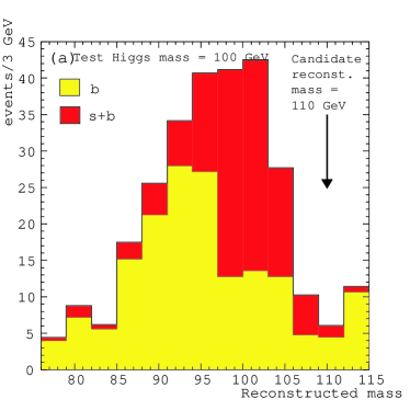
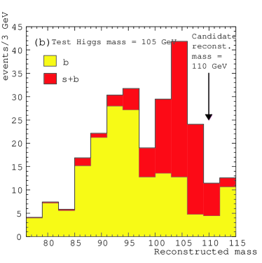
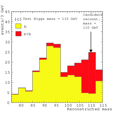
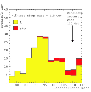
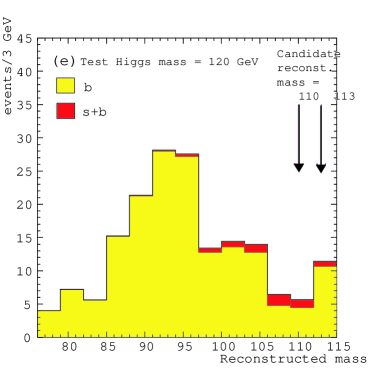
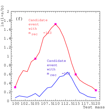
Figure 2: The ”spaghetti” curves represent the evolution of the event weight $\ln(1+s/b)$ with test mass $m_{H}$. The first five plots show the histograms of the signal (red) on top of the background (yellow) for test masses from 100-120 GeV. The arrow represent the location of the candidate reconstructed mass at $m_{H}=110$ GeV. The bottom right plot shows the resulting spaghetti plot for a candidate with $m_{rec}=110$ and $113$ GeV.

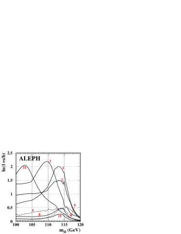
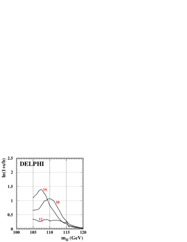
Figure 3: Evolution of the event weight $\ln(1+s/b)$ with test-mass $m_{H}$ for the events with the largest weight at $m_{H}=115$ GeV. The labels correspond to the candidate numbers in the first column of Table 1. The sudden increase in the weight of the OPAL missing-energy candidate labeled “13” at $m_{H}=107$ GeV is due to the switching from the low-mass to high-mass optimization of the search at that mass. A similar increase is observed in the case of the L3 four-jet candidate labeled “17” which is due to a test-mass dependent attribution of the jet-pairs to the Z and Higgs bosons.The Figure is taken from [2].

When does a Higgs candidate event become significant? What can be considered as a leading or gold plated Higgs candidate? Due to detector resolution and missing energy carried by undetected neutrinos which accompany the Higgs decay products, the reconstructed mass of a hypothetical Higgs candidate $m_{rec}$, is not necessarily its physical mass, $m_{H}$. One therefore defines a weight to quantify the significance of a Higgs candidate with $m_{rec}$ with respect to a hypothetical Higgs with $m_{H}$. This weight is given by $\ln(1+\frac{s(m_{H},m_{rec})}{b(m_{rec})})$ (see next section) where $s(m_{H},m_{rec})$ is the expected number of signal events from an hypothetical Higgs boson with a test mass $m_{H}$ in the vicinity of $m_{rec}$. This procedure is illustrated in a series of plots (Figure 2). In this example we assume there is an event candidate with a reconstructed mass, $m_{rec}=110$ GeV. We then calculate the event weight for hypothetical Higgs test masses in the range 100–120 GeV (Figs 2a-e). The resulting weights are shown in the last figure of this series (Fig. 2e). When connecting all the weights with a continuous line, one gets what has become to be known as the “spaghetti plot”. Also shown is the spaghetti plot for a candidate event with $m_{rec}=113$ GeV. As expected, the highest weight is achieved when the reconstructed mass and the hypothetical test Higgs mass coincide. The 17 candidates with the highest weight at a test mass, $m_{H}=115$ GeV are listed in Table 1 and their corresponding spaghetti plots are shown in Figure 3 (taken from [2]).

	Expt	$E_{cm}$	Decay channel	$m_{rec}$ (GeV)	$\ln(1+s/b)$
					at 115 GeV
1	ALEPH	206.6	4-jet	114.1	1.76
2	ALEPH	206.6	4-jet	114.4	1.44
3	ALEPH	206.4	4-jet	109.9	0.59
4	L3	206.4	E-miss	115.0	0.53
5	ALEPH	205.1	Lept	117.3	0.49
6	ALEPH	206.5	Taus	115.2	0.45
7	OPAL	206.4	4-jet	111.2	0.43
8	ALEPH	206.4	4-jet	114.4	0.41
9	L3	206.4	4-jet	108.3	0.30
10	DELPHI	206.6	4-jet	110.7	0.28
11	ALEPH	207.4	4-jet	102.8	0.27
12	DELPHI	206.6	4-jet	97.4	0.23
13	OPAL	201.5	E-miss	108.2	0.22
14	L3	206.4	E-miss	110.1	0.21
15	ALEPH	206.5	4-jet	114.2	0.19
16	DELPHI	206.6	4-jet	108.2	0.19
17	L3	206.6	4-jet	109.6	0.18

Table 1: Properties of the candidates with the highest weight at $m_{H}=115$ GeV. Table is taken from [2].

3 Understanding Likelihood Plots

At the end of the day, LEP is one big experiment with one experimental result. An experimental result is in this sense a configuration of data events that agree to some level the expectation from either a pure background (b) hypothesis or signal plus background (s+b) hypothesis (at some Higgs mass). Here we illustrate how the likelihood ratio is used to rank an experimental result between either being b-like or s+b-like.

The first step in telling a b-like from an s+b-like result is to construct a discriminator. Such a discriminator could be the reconstructed mass (obviously a peak at the reconstructed mass on top of the background will indicate a “signal observation”). It could also be a 2-D discriminator, where the other discriminating variable is, for example, the b-tag content of an event. The Higgs, being the generator of particle masses, decays dominantly to b-quarks in this mass range. In our toy model, we use the reconstructed mass as a discriminator.

Once the discriminator is defined, we divide it into bins, $i=1,2,.....,N_{bins}$ each containing $N_{i}$ observed candidates. The likelihood ratio $-2\ln Q(m_{H})$ tells us how much the outcome of an experiment is signal-like [5]. It is given by

$$Q=\frac{P_{Poisson}(Data|s+b)}{P_{Poisson}(Data|b)}=\frac{L(s+b)}{L(b)}=\frac{\exp(-(s_{TOT}+b_{TOT}))}{\exp(-b_{TOT})}\prod_{i=1}^{N_{bins}}\left({\frac{s_{i}+b_{i}}{b_{i}}}\right)^{N_{i}},$$ (1)

which is easily simplified to

$$-2\ln Q(m_{H})=2s_{TOT}-2\sum_{i=1}^{N_{bins}}N_{i}\ln\left(1+\frac{s_{i}(m_{H})}{b_{i}}\right),$$ (2)

which is a weighted sum of all the observed events.

Next we demonstrate how to construct the Probability Density Function (p.d.f.) of the likelihood for an ensemble of background and signal+background experiments.

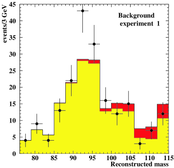
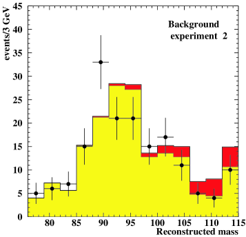
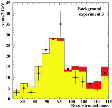
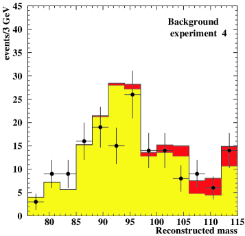
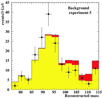
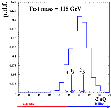
Figure 4: The first five plots show the histograms of the 115 GeV Higgs signal (red) on top of the background (yellow) for a Higgs test mass of 115 GeV. The dots with error bars represent a simulated data of random background only experiments. Each experiment yields a likelihood represented by the arrows in the bottom right plot. By performing an infinite number of background only experiments one gets the probability density function shown in the bottom right plot.

The histograms in Figure 4 show the expected background and 115 GeV Higgs signal (on top of the background) distributions of the discriminating variable, here taken to be the reconstructed mass. We then show five possible outcomes of experiments, all generated without the signal. The experiments are numbered 1–5. For each experiment we use the observed events configuration ($N_{i}$) and the hypothetical Higgs test mass $m_{H}$ to calculate the likelihood $-2\ln Q(m_{H})$ following equation 2. The resulting likelihoods are shown at the bottom right plot. Only experiment 4 has some excess of events at the high mass region which results in an s+b-like likelihood. The other 4 experiments result in a b-like likelihood. The likelihood p.d.f. is the histogram generated when performing a large number of background only experiments. As one can see (from simple areas considerations), in this “typical” toy example , the probability for a b-only experiments to give a s+b-like likelihood is about 15% (not so small…).

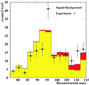
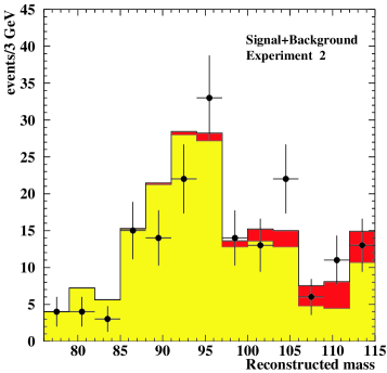
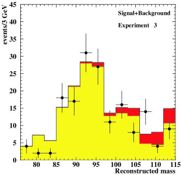
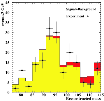
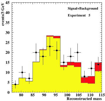
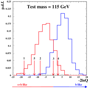
Figure 5: The first five plots show the histograms of the 115 GeV Higgs signal (red) on top of the background (yellow) for a Higgs test mass of 115 GeV. The dots with error bars represent simulated data of random signal+background experiments. Each experiment yields a likelihood represented by the arrows in the bottom right plot. By performing a large number of signal+background only experiments one gets the probability density function(p.d.f.) shown in the bottom right plot. Also shown is the background only p.d.f.

The same procedure was repeated for signal+background experiments (see Figure 5). The bottom right plot shows the likelihood of the five numbered s+b experiments. As one can see, experiments 3 and 4 gave a background-like likelihood. Repeating the s+b experiments a large number of times yielded another p.d.f. from which we see that in this specific toy example, there is about a 20% probability for a 115 GeV signal to give a b-like event configuration. The p.d.f’s of the s+b and b-only experiments give us an indication of the discriminating power of the likelihood.

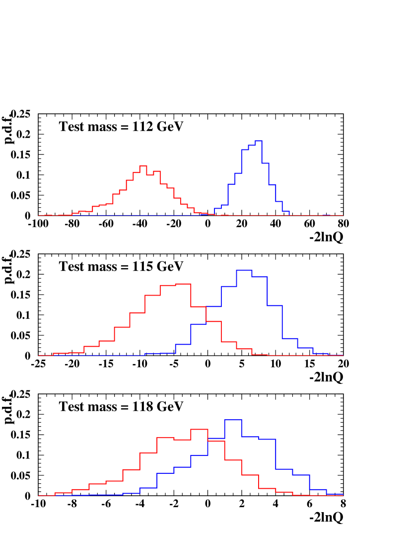
Figure 6: The separation between the Signal and the Background for various Higgs masses is shown by their likelihood p.d.f’s.

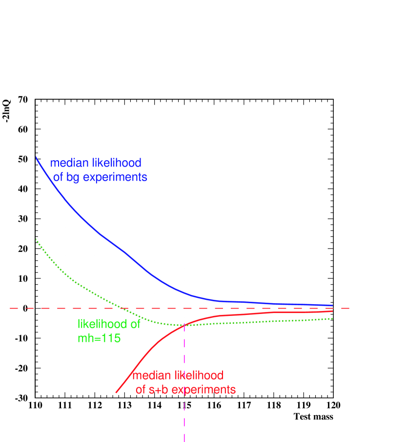
Figure 7: Median expected likelihood of background-only (blue), signal(at the test mass $m_{H}$)+background (red) and a fake 115 GeV Higgs signal (green) as a function of the test Higgs mass $m_{H}$.

This is illustrated in Figure 6 where the p.d.f’s of b-only and s+b experiments are shown for $m_{H}=112,115$ and $118$ GeV. For the lighter Higgs, the production cross section is high allowing a good separation between signal and background. For the heavier Higgs the signal production cross section is very low resulting in a weak separation. The dependence of the likelihood on the hypothetical test Higgs mass is illustrated in Figure 7 where the median of the p.d.f. distributions is shown for b-only and s+b experiments. As the Higgs test mass increases the signal and background separation power decreases resulting in a reduced discovery potential. This median can serve as a reference measure to the signal-like nature of the experimental result. To demonstrate this, we planted into our background Monte Carlo sample a 115 GeV Higgs boson signal. We then generated the p.d.f. of this fake signal likelihood. The resulting p.d.f. median is also shown in Figure 7. One can see, as expected, that this likelihood reaches a broad minimum at a test mass in the vicinity of $m_{H}=115$ GeV. Naturally, this likelihood coincides with that of the s+b experiments for a test mass of 115 GeV.

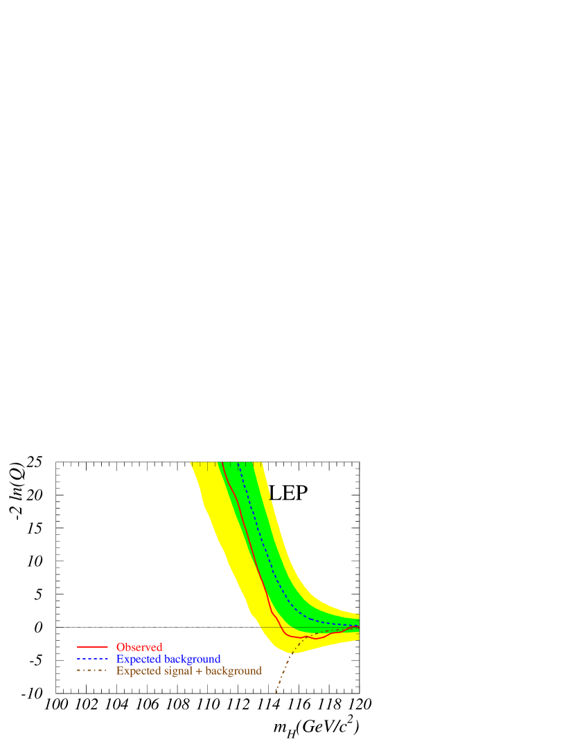
Figure 8: Observed and expected behavior of the likelihood $-2\ln Q$ as a function of the test-mass $m_{H}$ for combined LEP experiments. The solid/red line represents the observation; the dashed/dash-dotted lines show the median background/signal+background expectations. The dark/green and light/yellow shaded bands represent the 1 and 2 $\sigma$ probability bands about the median background expectation [2].

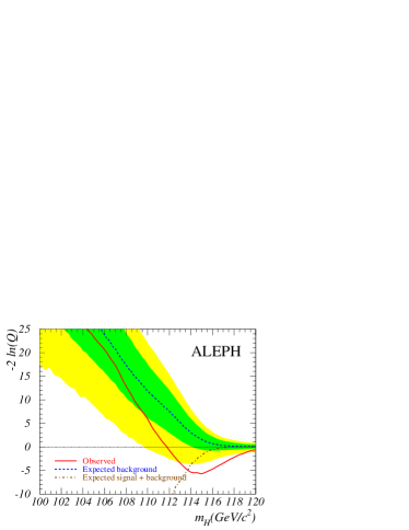
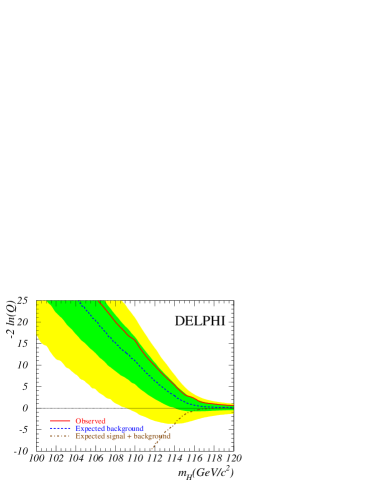
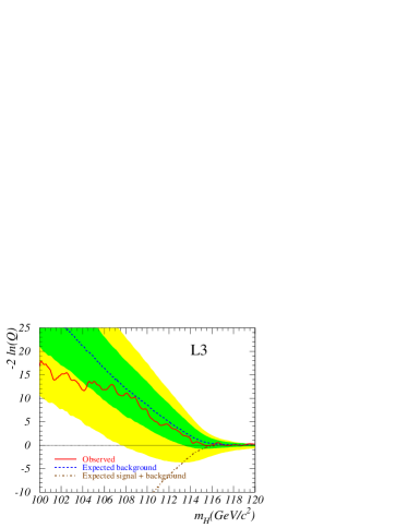
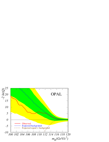
Figure 9: Observed and expected behavior of the likelihood $-2\ln Q$ as a function of the test-mass $m_{H}$ for the various experiments. The solid/red line represents the observation; the dashed/dash-dotted lines show the median background/signal+background expectations. The dark/green and light/yellow shaded bands represent the 1 and 2 $\sigma$ probability bands about the median background expectation [2].

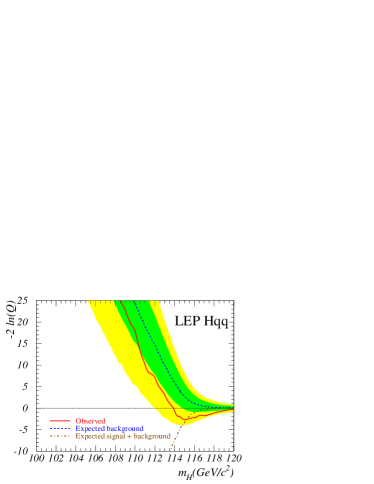
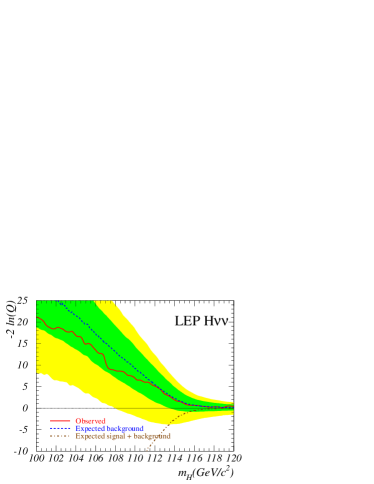
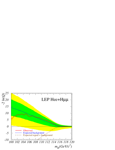
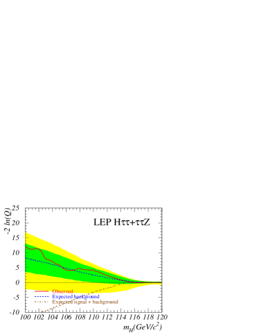
Figure 10: Observed and expected behavior of the likelihood $-2\ln Q$ as a function of the test-mass $m_{H}$ for the various Higgs search channels. The solid/red line represents the observation; the dashed/dash-dotted lines show the median background/signal+background expectations. The dark/green and light/yellow shaded bands represent the 1 and 2 $\sigma$ probability bands about the median background expectation [2].

Now that we have learned how to read the likelihood plots let us examine the LEP experimental outputs [2]. The likelihood outcome of the combined four LEP experiments is shown in Figure 8. This result can be sliced into the different experiments (Figure 9) or the different search channels (Figure 10)[2]. Shown are the b-only median expectations with its 1 and 2$\sigma$ bands, the s+b expectation and the observed likelihood. The broad minimum of the combined LEP likelihood from $m_{H}\sim 115-118$ GeV which crosses the expectation for s+b around $m_{H}\sim 116$ GeV can be interpreted as a preference for a Standard Model Higgs boson at this mass range, however, at less than the 2$\sigma$ level. When the LEP Higgs working group presented these results for the first time the significance was 2.9$\sigma$ [1], and this relatively high significance generated a storm which unfortunately turned out to be in a tea cup…

The ALEPH observed likelihood has a 3$\sigma$ signal-like behavior around $m_{H}\sim$ 114 GeV, which led the collaboration to claim a possible observation of a SM Higgs boson [3]. This behavior originated mainly from the 4-jet channel and its significance is reduced when all experiments are combined. No other experiment or channel indicated a signal-like behavior.

4 Confidence Levels or How Probable is a Result?

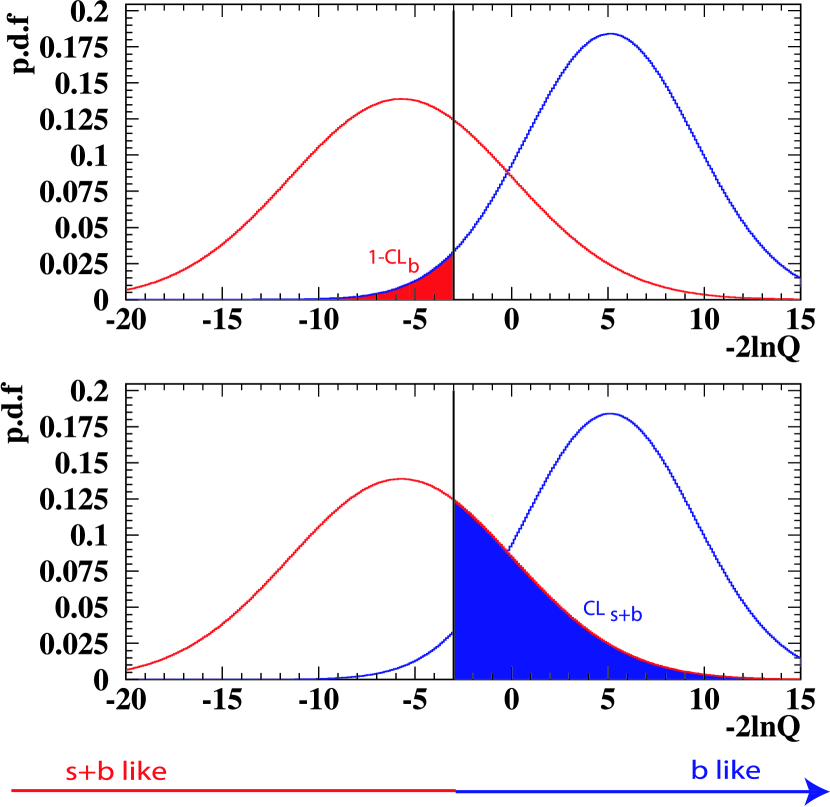
Figure 11: An example of probability density functions (p.d.f’s) for background only (solid blue) and signal+background (solid red) experiments. The red shaded area, $1-CL_{b}$, measure the compatibility with the background hypothesis while the blue shaded area, $CL_{s+b}$, the compatibility with the signal+background hypothesis. Detailed explanations are given in the text.

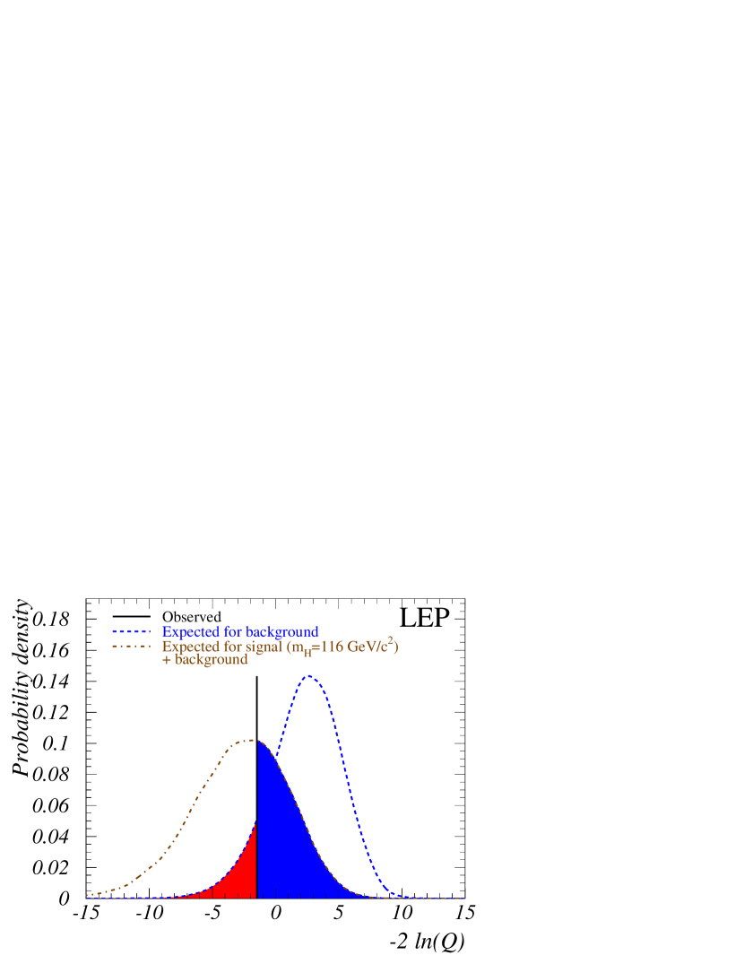
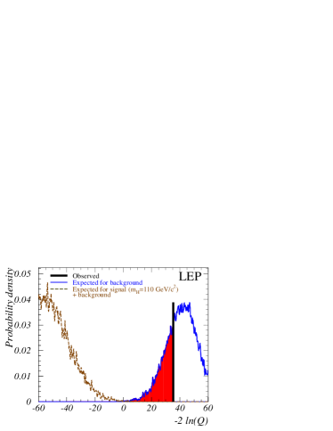
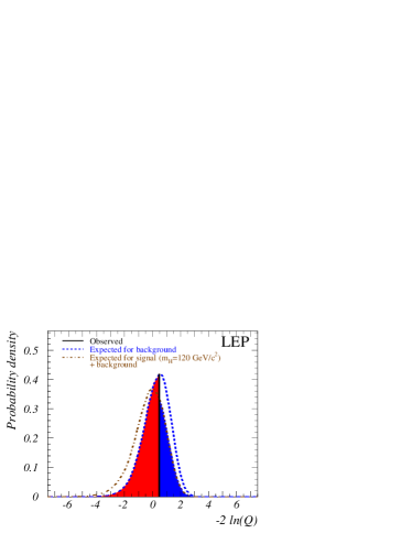
Figure 12: Probability density functions corresponding to fixed test-masses, for the background and signal+background hypotheses. The observed likelihood ratio $-2\ln Q$ is indicated by the vertical line. The light/red shaded areas, $1-CL_{b}$, measure the compatibility with the background hypothesis and the dark/blue shaded areas, $CL_{s+b}$, the compatibility with the signal+background hypothesis. Upper part: test-mass $m_{H}=116$ GeV; lower part: $m_{H}=110$ (left) and $120$ GeV (right) [2].

Figure 11 shows the likelihood p.d.f. of our toy model with a test mass of $m_{H}\sim 115$ GeV. Assuming an hypothetical observed likelihood of $-2\ln Q=-3$ the probability for a b-only experiment to give a more s+b-like likelihood than the observed one is given by the area marked as $1-CL_{b}$, where $CL_{b}$ is the background confidence level. It is easy to see that the expectation value of this probability is 50%, i.e. $\langle 1-CL_{b}\rangle=0.5$ irrespective of the test Higgs mass. One might also say that $CL_{b}$ measures the compatibility with the background hypothesis. The combined LEP p.d.f. is given in Figure 12. For a test mass of $m_{H}=116$ GeV, the observed likelihood is such that $1-CL_{b}=0.099$ [2], i.e., in 9.9% of background-only experiments, we expect to observe a result at least as signal-like as we observe. In the bottom plots of this Figure, the p.d.f’s are shown for Higgs test masses of 110 and 120 GeV where the observed probability is clearly consistent with the background hypothesis. These probabilities can be translated into a significance. A Gaussian approximation is used [4]. Table 2

$1-CL_{b}$	$0.32$	$0.046$	$2.7\times 10^{-3}$	$6.3\times 10^{-5}$	$5.7\times 10^{-7}$
	1$\sigma$	2$\sigma$	3$\sigma$	4$\sigma$	5$\sigma$

Table 2: Significances

shows the correspondence between $1-CL_{b}$ and the resulting significance. Therefore, the combined LEP observed likelihood corresponds to a significance below 2$\sigma$.

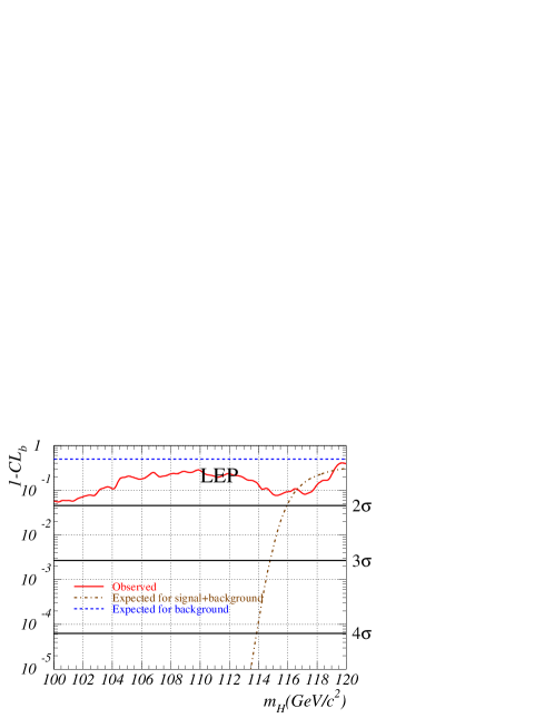
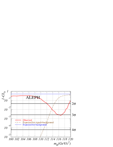
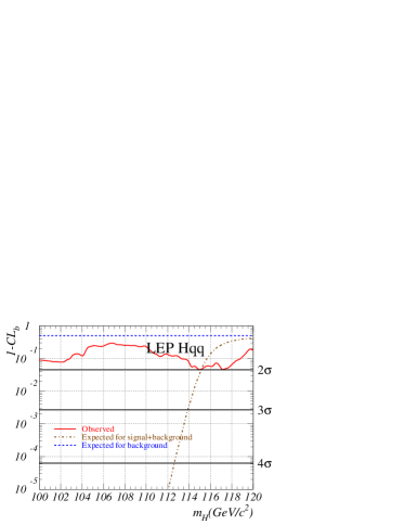
Figure 13: Probability $1-CL_{b}$ as a function of the test-mass $m_{H}$. Solid/red line: observation; dashed/dash-dotted lines: expected probability for the background/signal+background hypotheses. The horizontal solid lines indicate the levels for 2$\sigma$, 3$\sigma$ and 4$\sigma$ deviations from the background hypothesis. The top plot is the combined LEP result while the bottom plots show the ALEPH and the LEP 4-jet channel results[2].

Figure 13 (top) shows the probability $1-CL_{b}$ as a function of the test mass $m_{H}$ [2]. Shown are the median probability expected for b-only (dashed) and s+b (dash-dotted) experiments, and the observed probability (solid red line). One can see that even though the observed probability is compatible with a $\sim$116 GeV Higgs boson, the sensitivity in this vicinity is less than 2$\sigma$, and LEP did not really have the sensitivity to observe a Higgs boson heavier than 115 GeV with more than 3$\sigma$ significance (this can be seen by the intersection of the dash-dotted line with the horizontal 3$\sigma$ line). In fact, The LEP sensitivity to observe a SM Higgs boson at greater than 3$\sigma$ significance extends up to about 115 GeV and up to about 116 GeV for observation at greater than 2$\sigma$.

The bottom plots of Figure 13 show the probability $1-CL_{b}$ where the ALEPH excess of candidate events in the 4-jet channel manifests itself as a 3$\sigma$ deviation for a 116 GeV Higgs boson for ALEPH alone, and a 2$\sigma$ deviation in the combined LEP 4-jet channel. Note that ALEPH stand-alone sensitivity to observe a Higgs boson at the 3$\sigma$ level extends up to $m_{H}\sim 113$ GeV, which is of course less than the combined LEP sensitivity. The ALEPH excess should therefore be interpreted as a fluctuation in that context.

In case there are no clear indications for discovery, one would like to interpret the search results in terms of exclusion. The probability $CL_{s+b}$, shown as the blue area in the bottom plot of Figure 11, measures the compatibility of the experiment with the s+b hypothesis. There is no way to directly measure the signal Confidence Level, $CL_{s}$ because of the presence of significant background. A bigger $CL_{s+b}$ means the experimental result is more s+b-like, but not necessarily more s-like due to the relative fluctuations of the background. Therefore, if $CL_{s+b}$ is small, say, less than 5%, one can exclude the s+b hypothesis at more than 95% Confidence Level, but that does not mean that the signal hypothesis is excluded at that level. An example is given in Table 3 [2]

	$1-CL_{b}$	$CL_{s+b}$
LEP	0.099	0.369
ALEPH	$2.41\times 10^{-3}$	0.956
DELPHI	0.874	0.033
L3	0.348	0.408
OPAL	0.543	0.208
Four-jet	$5.70\times 10^{-2}$	0.676
All but four-jet	0.368	0.217

Table 3: The background confidence level $1-CL_{b}$ and the signal+background confidence level $CL_{s+b}$ at $m_{H}=116$ GeV, for all LEP data combined and for various subsets of the data. The numbers for the four-jet and all-but-four-jet final states are obtained with the data of the four experiments combined. Table taken from [2].

where the background confidence level $1-CL_{b}$ and the signal+background confidence level $CL_{s+b}$ at $m_{H}=116$ GeV, for all LEP data combined and for various subsets of the data are shown . Note that the DELPHI $CL_{s+b}$ probability is 3.3%. That does not mean that DELPHI could exclude a 116 GeV Higgs boson signal hypothesis, but rather that DELPHI can exclude a 116 GeV s+b hypothesis. However, there is a $1-CL_{b}=87.4\%$ probability for the DELPHI background to fluctuate and give a signal-like observation. It was to take this probability into account that one apriori defined the signal Confidence level to be $CL_{s}=\frac{CL_{s+b}}{CL_{b}}$ [5]. This way the signal hypothesis for $m_{h}=116$ GeV is excluded by definition at only the 73.8% Confidence Level, $CL=1-CL_{s}=1-0.033/0.126=0.738$. This procedure for constructing the signal confidence level is obviously conservative since the coverage probability is in general greater than the $CL$.

Of the three plots shown in Figure 12 it is clear now that a 110 GeV Higgs boson, where the $CL_{s+b}$ probability is too small to be seen, can be excluded by LEP. This is also seen in Table 3 where none of the experiments alone or the combined LEP can exclude a 116 GeV Higgs boson.

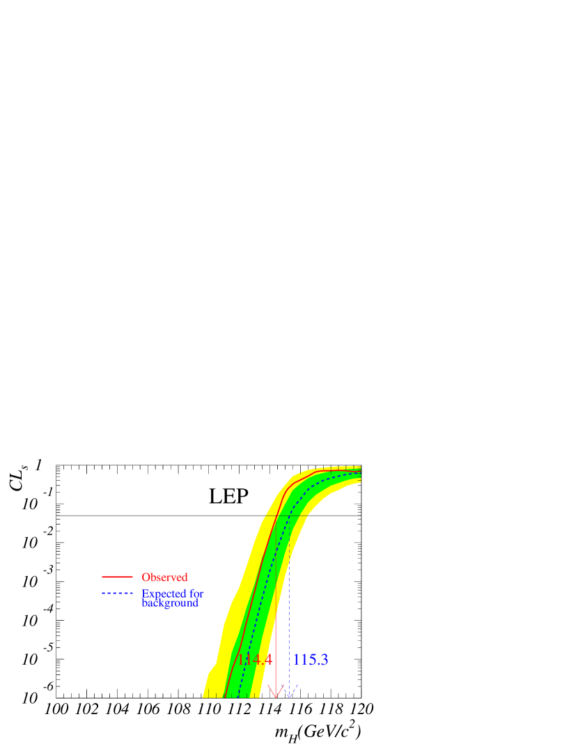
Figure 14: Confidence level $CL_{s}$ for the signal+background hypothesis. Solid/red line: observation; dashed line: median background expectation. The dark/green and light/yellow shaded bands around the median expected line correspond to the 1 and 2 $\sigma$ probability bands computed with a large number of simulated background experiments. The intersection of the horizontal line at $CL_{s}=0.05$ with the observed curve defines the 95% confidence level lower bound for the mass of the Standard Model Higgs boson[2].

The exclusion power of LEP is illustrated in Figure 14 [2] where the median expected signal confidence level, $\langle CL_{s}^{\rangle}$, as a function of the Higgs test mass together with its 1 and 2$\sigma$ bands is shown. Also shown is the observed $CL_{s}$ confidence level. The intersection of the horizontal line at $CL_{s}=5\%$ with the observed and median expected curves give the 95% observed and expected exclusion CL. Thus LEP excluded, at 95% CL, a SM Higgs boson with a mass below 114.4 GeV, while it had the sensitivity to exclude a 115.3 GeV Higgs boson. The small excess of data candidate events around 115–116 GeV is responsible for the slight reduction of the observed Higgs lower mass limit with respect to its potential exclusion sensitivity.

5 Conclusion

LEP Standard Model Higgs search results were reviewed with the emphasis on a pedagogical explanation of the statistical procedure based on a toy model constructed specifically for this purpose.

6 Acknowledgements

We would like to thank Moshe Kugler , Rick Van Kooten and Alex Read for their useful suggestions and illuminations after a critical reading of this note. One of the authors (E.G.) would like to thank the following people: Peter Zerwas for inviting him to summarize the LEP Higgs status in SUSY02 at DESY Hamburg, and thereby initiating this work; Alex Read for teaching him everything he knows about Higgs statistics, Chris Tully for giving him a private LEP Higgs statistics lesson and Inbar Mor for the good vibes and support while completing this work.

References

-
[1]
P. Igo-Kemenes, presentation to the LEPC, Nov 3, 2000,
http://lephiggs.web.cern.ch/LEPHIGGS/talks/pik_lepc_nov3_2000.ps -
[2]
Search for the Standard Model Higgs Boson at LEP, ALEPH, DELPHI,
L3 and OPAL, the LEP Working Group for Higgs Boson Searches,
Contributed paper for ICHEP’02 (Amsterdam, July
2002),
http://lephiggs.web.cern.ch/LEPHIGGS/papers/July2002_SM/index.html - [3] Final results of the searches for neutral Higgs bosons in collisions at up to 209 GeV / Heister, A ; et al. - ALEPH Collaboration. hep-ex/0201014 ; CERN-EP-2001-095. - Geneva : CERN , 18 Dec 2001. - 19 p. Phys. Lett., B : 526 (2002) , pp.191-205
- [4] D. E. Groom et. al., Euro. Phys. Journ. C15(2000) 1.
-
[5]
A.L. Read, Nucl. Instr. Methods A 425 (1999) 357.
A. Read, in 1st Workshop on Confidence Limits, CERN-2000-005.