Recent Results from the K2K Experiment

Abstract

The K2K experiment has collected approximately half of its allocated protons on target between June of 1999 and July of 2001. These proceedings give a short introduction to the experiment and summarize some of the recent results.

1 INTRODUCTION

The K2K experiment uses an accelerator produced neutrino beam with a long baseline between the production of the neutrinos and their detection to search for neutrino oscillations. The goal of the K2K experiment is to confirm the atmospheric neutrino oscillation effect by observing neutrino oscillation over the 250 km distance between KEK and Super-Kamiokande.

2 EXPERIMENTAL DETAILS

The neutrino beam used in the K2K experiment is produced by a 12 GeV proton beam taken from the KEK Proton Synchrotron(PS) with fast extraction. After hitting an aluminum target the positively charged particles, mostly pions, are focused by a pair of horns. The beam is approximately 98% muon neutrino with a 2% electron neutrino contamination. The peak energy of the resulting neutrinos is 1 GeV, with a mean energy of 1.4 GeV. The beam pulse is extracted from the PS in a single turn every 2.2 seconds with a pulse structure of 9 bunches in 1.1 $\mu$sec.

The pion beam’s momentum and divergence is occasionally monitored by a gas Cherenkov monitor downstream of the second horn. These measurements are used to confirm the correctness of the beam MC. The beam MC is used to predict the neutrino flux at Super-K given the measurements at the near detector at the point of neutrino production. Figure 1 shows both the measured and predicted ratio of neutrino fluxes at the far and near detectors using the pion monitor.

Figure 1: Ratio of the neutrino spectrum at Super-K and the near detectors as predicted by the beam MC and measured by the pion monitor for neutrino energies above 1 GeV.

The near detector of the K2K experiment is 300 m downstream of the beam target. The near detector is comprised of two detector systems: a 1 kt water Cherenkov tank and a fine-grained tracking system. Figure 2 is a schematic representation of the near detector. The 1 kt water Cherenkov detector is a scaled down version of the Super-Kamiokande detector. Its main purpose is to use the same method of detecting events at both the near and far detector sites. In this way, systematic errors or biases introduced by using a water Cherenkov detector will be canceled in a direct comparison of measurements in the near and far detectors. It is also desirable to make precision measurements of the transverse profile, energy distribution, and $\nu_{e}$ contamination of the neutrino beam at the near detector. For this reason, a fine-grained detector is also employed. We also hope to measure exclusive neutrino reactions on water such as single-$\pi$ production. The fine-grained detector consists of a scintillating fiber tracker, trigger counters, lead glass counters and a muon ranger.

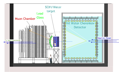
Figure 2: The near detector of the K2K experiment. The detector is compromised of a 1 kt water Cherenkov detector, a scintillating-fiber water-target calorimeter, a lead-glass calorimeter, and a set of muon rangers. The experimental hall is cylindrical with a 24 m diameter and a depth of 16 m.

The lead glass counters are used to determine the $\nu_{e}$ contamination in the $\nu_{\mu}$ beam. Electrons produced by electron neutrinos shower in the lead glass and their energy can be measured with a resolution of 8%/$\sqrt{E_{e}}$. Muons, on the other hand, are minimum ionizing and leave less than $\sim$ 1 GeV. The reason it is important to measure accurately the amount of contamination by electron neutrinos is that unmeasured $\nu_{e}$s in the neutrino beam might be interpreted at the far detector as evidence for $\nu_{\mu}\rightarrow\nu_{e}$ oscillation. A preliminary analysis has shown a measured electron contamination consistent with the expectation of $\approx$ 2%.

Finally, the muon rangers are made of 12 iron plates instrumented with drift tubes. They are used to measure the momentum of muons generated by charged current interactions in the water target of the fiber tracker. Also because of the large mass of the iron there is a very large contained event rate which allows us to measure the neutrino beam center and profile as a function of time. Figure 3 shows the horizontal and vertical beam profiles as measured in the muon chambers and also the peak position as measured every five days. This measurement confirms the the beam direction is stable to within 1 mrad.

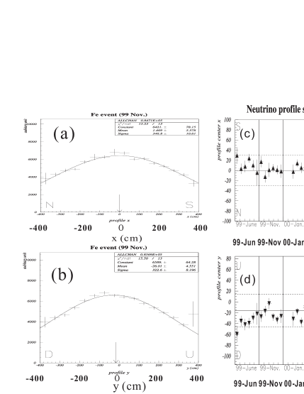
Figure 3: Horizontal and vertical beam profiles as measured by muon chambers. Also shown are the peak positions as a function of time. The position is plotted on a time scale of every five days. The solid line shows the direction to Super-K and the dashed lines show a $\pm$1 mrad deviation.

2.1 CURRENT STATUS AND RESULTS

By comparing the GPS time stamps of proton beam spills at KEK and Super-K triggers we search for events that have arrived at Super-K within 1.1 usec of the the beginning of the neutrino pulse. Two classes of events are reconstructed at Super-K. The first, known as “Fully-Contained(FC)” are events where all of the Cherenkov light in the event is contained in the inner detector of Super-K. The second class of events are known as “outer detector(OD)” events since Cherenkov light is also seen in the outer detector.

The FC events are further sub-divided into events which fall inside of the 22.5 kton fiducial volume(FC-in) and those that fall outside(FC-out). Since the Super-K reconstruction algorithms are, at this time, only guaranteed to work inside of the fiducial volume we only use the FC-in events for quantitative analysis.

By using the measured neutrino rates in the near detectors and the ratio of near to far fluxes as calculated by the beam MC we predict how many events should be seen at Super-K. The number predicted in the fiducial volume of Super-K by the near detectors for our present running period is: $N_{SK}^{pred}\ =80.1^{+6.2}_{-5.4}$, compared to 56 events detected. The number of observed events are summarized in Table 1.

Table 1: Observed number of events in the fiducial volume at SK.

single ring	$\mu$-like	30
	e-like	2
multi ring		24
Total		56

Figure 4 shows the time difference of the FC events between the KEK accelerator beam time and the time of the trigger in Super-K corrected for the time of flight of the neutrinos. The FC events in the fiducial volume are shown in the lower figure and all of the events clearly fall within the 1.1 $\mu$sec beam window.

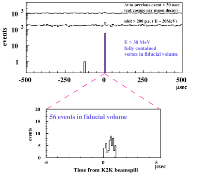
Figure 4: Beam Spill time - SK time - TOF for FC events in Super-K. The upper figure shows a simplified view of the K2K data reduction. The lower figure shows the events detected in the fiducial region of Super-K. All events fall in the beam window.

Although fully-contained events will provide the cleanest sample of beam-induced neutrinos, we are also looking for neutrinos that interact in the Super-K outer detector, or in the rock outside the detector. This has the potential to increase the number of events usable in the oscillation analysis. More importantly, it provides an important cross check of beam stability during periods when a low statistics fluctuation suggests a gap in the data; evidence of OD events indicates that any gap in the golden inner detector event sample is statistical in nature. In Fig. 5 the arrival time of Super-K events is plotted versus integrated luminosity. The arrival times of the events are consistent with a Poisson distributed distribution.

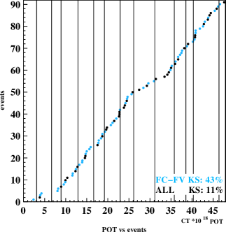
Figure 5: Arrival time of each far-detector event versus accumulated protons-on-target. Light blue circles represent the cleanest events: fully-contained with vertex in the fiducial volume. The dark blue circles includes out-of-fiducial-volume events.

In addition to a reduction in the number of events seen, in the case of oscillations we expect to see a spectral distortion. We can estimate the neutrino energy for single-ring events from quasi-elastic scattering. Since the direction of the incoming neutrino is known, by measuring the momentum and scattering angle of the single muon ring, the energy of the neutrino can be calculated.

3 OSCILLATION ANALYSIS

The oscillation analysis is performed by the maximum-likelihood method. The major features of the analysis are that both the spectral shape information at SK and the number of observed events at SK are used. Also, correlations between energy bins in the neutrino spectrum along with correlation in the far/near ratio are taken into account.

The criteria used to select the neutrino events in SK have been described in detail elsewhere [1]. The basic selection criteria are that events must have no activity in the outer detector, have an electron equivalent energy greater than 30 MeV, and have a vertex reconstructed inside of the 22.5 kton fiducial volume. In order to predict the number of events and neutrino spectrum observed in SK, the number of events observed in the 1kt detector and the spectrum measured in all of the near detectors were extrapolated to 250 km away by using the far/near spectrum ratio estimated by the MC and the pion monitor measurements. In this way, the systematic error on the the predicted number of events is greatly reduced thanks to the similar efficiencies of the 1kt and SK and the fact that they both contain a water target.

3.1 Description of the analysis techniques

In order to extract the maximum amount of information about the mixing parameters from the 56 events detected in the fiducial volume of Super-Kamkiokande we performed an unbinned maximum likelihood analysis, comparing the data with MC expectation. For the single-ring events in Super-Kamkiokande, where the energy of the incoming neutrino can be easily estimated, both the shape of the energy spectrum and the total number of events which were detected were considered in the likelihood function. For the all other events, where QE kinematics can’t be used to estimate the neutrino energy, only the total number of detected and expected events are compared.

The likelihood is composed of the product of these two observables. ${\cal L}(\Delta m^{2},\sin^{2}2\theta)={\cal L}_{norm}(\Delta m^{2},\sin^{2}2\theta)\times{\cal L}_{shape}(\Delta m^{2},\sin^{2}2\theta)$. The normalization term is just the Poisson probability to observe $N_{obs}$ when expected number of events is $N_{exp}(\Delta m^{2},\sin^{2}2\theta)$. The shape term is the product of the probabilities that each event will have the measured reconstructed neutrino energy if it was drawn from the energy spectra as estimated by our MC simulation. These two terms are correlated since a distortion in the spectrum results in a decrease in the total number of events. In addition, the MC expectation is a function of a set of systematic error parameters. Uncertainties on the measured neutrino flux, far/near ratio etc will effect the expectation at Super-K.

The basic form of the likelihood is then:

$${\cal L}={\mu^{N_{obs}}e^{-\mu}\over N_{obs}!}\prod_{i=1}^{N_{1R}}p_{i}(E_{i},\Delta m^{2},\sin^{2}2\theta),$$ (1)

where $\mu$ is the expected rate of total observed events at this $\Delta m^{2}$ and $\sin^{2}2\theta$, $N_{obs}$ is the number of total events actually observed, $N_{1R}$ is the number of single-ring events, and $p_{i}$ is the probability of the $i^{th}$ event having the energy $E_{i}$ at a particular set of oscillation parameters.

In order to make allowed regions we calculated $\cal{L}$ over the space of oscillation parameters $\Delta m^{2}$ and $\sin^{2}2\theta$. In order to incorporate the systematic errors into this procedure two complimentary techniques were used. The first method uses numerical propagation of the systematic errors. The error matrices that were determined for the near detector flux, the near far extrapolation, and the shape and normalization as measured at Super-Kamkiokande were used to generate a set of Gaussian random correlated systematic error numbers which were then applied to our MC expectation. For example, the measured neutrino flux was sampled within its fitted errors which changes the expectation for the measured spectral shape at Super-K. This procedure was repeated 500 times at each point in the oscillation space and values of the likelihood were averaged so that the resulting likelihood was the likelihood sampled properly over the systematic error parameters. In this way the likelihood was sampled properly with all the correlations between the systematic error parameters taken into account.

The other technique used to include systematic errors was to modify the likelihood by adding constraint terms associated with each set of systematic error parameters. In this case the form of the likelihood becomes:

$${\cal L}_{sys}={\cal L}\times\prod_{i=0}^{N_{par}}e^{\left(\Delta{\bf f}^{T}_{i}\cdot{\bf M}^{-1}_{i}\cdot\Delta{\bf f}_{i}\right)},$$ (2)

where $\cal L$ is from Eqn 1, $N_{par}$ is the number of systematic error matrices, ${\bf M}$ is each error matrix, and $\Delta{\bf f}_{i}={\bf f}_{i}-{\bf f}_{i}(default)$ is the vector of systematic parameters associated with that matrix where ${\bf f}(default)$ is the default value of the parameter without any modification. At each point in the oscillation parameter space the systematic error parameters are varied in the constraints and in the main part of the likelihood until the total likelihood is minimized.

The set of systematic errors which were considered for this analysis included the spectrum measurement at the near detectors, the non-QE/QE cross-section ratio, and the far/near flux ratio. These errors are dependent on energy and are represented by a set of matrices with the full energy correlations included. In addition there are errors which represent the fiducial volume error in the 1kt and SK, the uncertainty on the energy scale of SK, and the uncertainty in the detection efficiency of SK.

The target radius and horn current, and hence, the neutrino spectrum in Jun 99 were different from those used in the rest of the running period. The full analyses of the near detector spectra and far/near ratio including all correlations has not yet been completed for this data period. Therefore, for ${\cal L}_{shape}$, the events in Jun 99 are not considered. For this reason 29 1-ring $\mu$-like events are used in the likelihood. For $L_{norm}$, the data of whole experimental period are used, i.e. $N_{obs}=56$.

3.2 Fit results

The ${\cal L}$ was calculated by either numerically propagating the systematic errors, or adding the likelihood constraint terms and minimizing the likelihood, at each point in the $\Delta m^{2}$ and $\sin^{2}2\theta$ space. Then, the point where the likelihood was maximized was located. The resulting best fit oscillation parameters are summarized in Table 2.

Table 2: Best fit points. The unit of $\Delta m^{2}$ is $10^{-3}$ eV². The results are shown for both the entire parameter space and for the case where the parameters are constrained to be physical.

	Likelihood		Numerical
	Constraint		Propagation
	$\sin^{2}2\theta$	$\Delta m^{2}$	$\sin^{2}2\theta$	$\Delta m^{2}$
Shape only	1.0	3.0	1.0	3.2
(allowing unphysical)	1.09	3.0	1.05	3.2
Norm + Shape	1.0	2.8	1.0	2.7
(allowing unphysical)	1.03	2.8	1.05	2.7

At the best fit point the total number of predicted events is 54.2(to be compared with the 56 observed). Using the single-ring $\mu$-like events as a fairly pure sample of quasi-elastic interactions, we measure the neutrino energy spectrum. The distribution of data is very low in second bin, from 500 MeV to 1 GeV. This is consistent with neutrino oscillations, as shown by the overlay of the best-fit spectrum in Fig. 6. The best-fit parameters are $\Delta m^{2}=2.7\times 10^{-3}{\rm eV}^{2}$ and $\sin^{2}2\theta=1$.

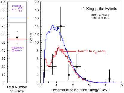
Figure 6: The total event count and single-ring $\mu$-like neutrino spectrum overlaid with expectations for no oscillations and oscillations at the K2K best fit point.

The consistency between the observed and best-fit reconstructed $E_{\nu}$ spectrum shown in Fig 6 was checked by the use of the KS test. A KS probability of 79% was obtained. Both our best fit number and shape agree very well with the observations.

3.3 The probability of the no oscillation hypothesis

The probability that our result is due to a statistical fluctuation instead of neutrino oscillation is calculated by computing the likelihood ratio of the best fit point to the no oscillation case. The results are 0.7% using the likelihood constraint method, and 0.4% for the method using the numerical propagation of errors. Finally, allowed regions of oscillation parameters for both methods are drawn in Fig. 7 along with the Super-K allowed region. The allowed regions from the two methods are consistent with each other as are the no-oscillation probabilities from the two methods.

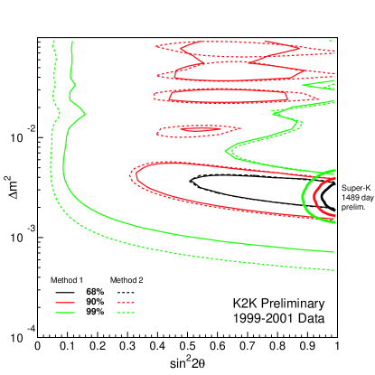
Figure 7: The confidence intervals based on the combined analysis of the total event rate plus the neutrino spectrum. The two methods refer to different treatments of systematic uncertainties.

Both methods give essentially the same results, the 90% CL contour crosses with the $\sin^{2}2\theta=1$ axis at $1.5$ and $3.9\times 10^{-3}$ eV². The results are clearly in agreement with the parameters found by the Super-Kamiokande atmospheric neutrino analysis. The probability that our data is a fluctuation from the no-oscillation hypothesis is less than 1%.

The K2K experiment has collected approximately one-half of its expected protons-on-target. We expect to begin new running in January of 2003.

References

- [1] S. H. Ahn, et al., Detection of accelerator produced neutrinos at a distance of 250-km, Phys. Lett. B511 (2001) 178–184.