Measurement of Branching Fractions in $\tau$ Decays

Abstract

Full LEP-I data collected by the ALEPH detector during 1991-1995 running are analyzed in order to measure the $\tau$ decay branching fractions. The analysis follows the global method used in the published study based on 1991-1993 data, with several improvements, especially concerning the treatment of photons and $\pi^{0}$’s. Extensive systematic studies are performed, in order to match the large statistics of the data sample corresponding to 327148 measured and identified $\tau$ decays. Preliminary values for the branching fractions are obtained for the 2 leptonic channels and 11 hadronic channels defined by their respective numbers of charged particles and $\pi^{0}$’s. Using previously published ALEPH results on final states with charged and neutral kaons, corrections are applied so that branching ratios for exclusive final states without kaons are derived. Some physics implications of the results are given, in particular concerning universality in the leptonic charged weak current, isospin invariance in $a_{1}$ decays, and the separation of vector and axial-vector components of the total hadronic rate.

1 Introduction

A complete and final analysis of $\tau$ decays is presented using a global method. All data recorded at LEP-I with the ALEPH detector are used, thus providing an update of those previous results which were based on partial data sets. The increase in statistics —the full sample corresponds to about 2.5 times the luminosity used in the last published global analysis [1, 2]— not only allows for a reduction of the dominant statistical error but, more importantly, provides a way to better study possible systematic biases and to eventually correct for them. Several improvements of the method have been introduced in order to achieve a better control over the most relevant systematic uncertainties: simulation-independent measurement of the $\tau\tau$ selection efficiency, improved photon identification especially at low energy where the separation between photons from $\tau$ decays and fake photons from fluctuations in hadronic or electromagnetic showers is delicate, a new method to correct the Monte Carlo simulation for the rate of fake photons, and stricter criteria for channels with low branching fractions. For consistency and in order to maximally profit from the improved analysis all data sets recorded from 1991 to 1995 have been reprocessed. The results presented in this paper thus supersede those already published in Ref. [3, 1, 2]. Only the measurements on final states containing kaons, which were already based on the full statistics, remain unchanged [6, 7, 8, 9].

2 Experimental method

2.1 The data and simulated samples

A detailed description of the ALEPH detector can be found elsewhere [10, 11].

Tau-pair events are simulated by means of a Monte Carlo program which includes initial state radiation computed up to order $\alpha^{2}$ and exponentiated, and final state radiative corrections to order $\alpha$ [12]. The simulation of the subsequent $\tau$ decays also includes single photon radiation for the decays with up to three hadrons in the final state. The longitudinal spin correlation is taken into account [13]. This simulation, with the detector acceptance and resolution effects, is used to initially evaluate the corresponding relative efficiencies and backgrounds. It also includes the tracking, the secondary interactions of hadrons, bremsstrahlung and conversions. For all these effects, detailed comparisons with relevant data distributions are performed and corrections to the MC-determined efficiencies are derived.

The data used in this analysis have been recorded at LEP I in 1991-1995. The numbers of detected $\tau$ decays are correspondingly 132316 in 1991-1993 and 194832 in 1994-1995, for a total of about $3.3\cdot 10^{5}$. The ratios between Monte Carlo and data statistics are 7.3 and 9.7 for 1991-1993 and 1994-1995 periods, respectively. Monte Carlo samples are generated for each year of data-taking in order to follow as closely as possible the status of the detector components.

2.2 Selection of $\tau\tau$ events

The principal characteristics of $\tau\tau$ events in $e^{+}e^{-}$ annihilation are low multiplicity, back-to-back topology and missing energy. Each event is divided into two hemispheres by an energy flow algorithm [11] which calculates all the visible energy avoiding double-counting between the TPC and the calorimeter information. The jet in a given hemisphere is defined by summing all the four-momenta of all energy flow objects (charged and neutral). The energies in the two hemispheres including the energies of photons from final state radiation, $E_{1}$ and $E_{2}$, are useful variables for separating Bhabha, $\mu\mu$ and $\gamma\gamma$-induced events from the $\tau\tau$ sample, while the relatively larger jet masses, wider opening angles, and higher multiplicities indicate $Z\rightarrow q\overline{q}$ events.

All these features are incorporated in a standard selector used extensively in ALEPH [14, 1, 2]. In the previous analyses [1, 2] additional cuts had been introduced in order to further reduce the contamination from $ee$ and $\mu\mu$ processes. In the present work it was chosen to simplify the procedure in order to conveniently measure selection efficiencies on the data, at the expense of a slightly larger background contamination which is anyway also measured in the data sample as explained later.

We use the ’break-mix’ method introduced for the determination of the $\tau\tau$ cross section [14] to measure the efficiency of all the selection cuts. For every cut, one hemisphere of the event is chosen judiciously so that it is unbiased with respect to the cut under study and free of non-$\tau$ backgrounds. This procedure selects the opposite hemisphere as an unbiased $\tau$ decay which is then stored away. Pairs of selected hemispheres are combined to construct a $\tau\tau$ event sample built completely from data. This sample is used to measure the efficiency of the given cut.

The measured efficiencies are found to be very close to those obtained by the simulation, deviations being at most at the few per mille level. This situation stems from the facts that the $\tau$ decay dynamics is —apart from small branching ratio channels— very well known, the selection efficiencies are large and the simulation of the detector is adequate. The overall selection efficiency of $\tau\tau$ events is 78.8 %. This value increases to 91.9 % when the $\tau\tau$ angular distribution is restricted to the detector polar acceptance, giving a better indication for the efficiency of the cuts designed to exclude non-$\tau\tau$ backgrounds. In addition, when expressed relatively to each $\tau$ decay, the selection efficiencies are weakly dependent on the final state, with a total relative span of only 10 % for the 13 considered decay topologies.

2.3 Estimation of non-$\tau\tau$ backgrounds

A new method —already implemented for the measurement of the $\tau$ polarization [15]— has been developed to directly measure in the final data samples the contributions from the major non-$\tau$ backgrounds: Bhabhas, $\mu^{+}\mu^{-}$ pairs, and $\gamma\gamma\rightarrow e^{+}e^{-},\mu^{+}\mu^{-}$, and hadrons events. The procedure does not require an absolute normalization from the Monte Carlo simulation of these channels, only a qualitative description of the distribution of the discriminating variables. The basic idea is to apply cuts on the data in order to reduce as much as possible the $\tau\tau$ population while keeping a high efficiency for the background source under study, i.e. the reverse of what is done in the $\tau\tau$ selection.

The non-$\tau$ backgrounds in each channel are listed in Table 1. They amount to a total fraction of ($1.23\pm 0.04$) % in the full data sample.

2.4 Charged particle identification

A ’good’ track is defined to have a momentum greater than or equal to 0.10 GeV/c , $|\cos(\theta)|\leq 0.95$, at least 4 hits in the TPC, and its minimum distance to the interaction point within 2 cm transversally and 10 cm along the beams. In classifying $\tau$ decays, only good tracks are used, after removing those identified as electrons which are used to reconstruct converted photons; the electrons identified as bad tracks are also included in the reconstruction of conversions.

Charged particle identification is achieved with a likelihood method incorporating the information from the relevant detectors. In this way, each charged particle is assigned a set of probabilities from which a particle type is chosen. No attempt is made in this analysis to separate kaons from pions in the hadron sample since final states containing kaons have been previously studied [6, 7, 8].

Eight discriminating variables are used in the identification procedure: $dE/dx$ in the TPC, two estimators (transverse and longitudinal) of the shower profile in ECAL, the average shower width measured with the HCAL tubes in the fired planes, the number of fired planes among the last ten, the energy measured with HCAL pads, the number of hits in the muon chambers ($\pm 4\sigma$-wide around the track extrapolation, where $\sigma$ is the standard deviation expected from multiple scattering), and finally, the average distance (in units of the multiple-scattering standard deviation) of the hits from their expected position in the muon chambers.

The performance of the particle identification has been studied in detail using control samples of Bhabha events, $\mu\mu$ pairs, $\gamma\gamma$-induced lepton pairs and hadrons from $\pi^{0}$-tagged $\tau$ decays over the full angular and momentum range [1]. Measured efficiencies and misidentification probabilities are given in Figs. 1 and 2.

Figure 1: Hadron identification efficiency and misidentification probabilities obtained from the $\tau\tau$ Monte Carlo, corrected from data using the control samples, for the 1994-1995 data set.

Figure 2: Lepton identification efficiencies obtained from the $\tau\tau$ Monte Carlo, corrected from data using the control samples, for the 1994-1995 data set.

2.5 Photon identification

The high collimation of $\tau$ decays at LEP energies quite often makes photon reconstruction difficult, since these photons are close to one another or close to the showers generated by charged hadrons. Of particular relevance is the rejection of fake photons which may occur because of hadronic interactions, fluctuations of electromagnetic showers, or the overlapping of several showers. These problems reach a tolerable level thanks to the fine granularity of ECAL, in both transverse and longitudinal directions, but nevertheless they require the development of proper and reliable methods in order to correctly identify photon candidates.

A cluster in ECAL is accepted as a photon candidate if its energy exceeds 300 MeV and if its barycentre is at least 2 cm away from the closest track extrapolation.

A likelihood method is used for discriminating between genuine and fake photons. For every cluster, an estimator $P_{\gamma}$ is defined, $P_{\gamma}=0,1$ corresponding to fake and real photons,respectively. It is constructed using probability densities obtained by simulation, but corrected through detailed comparisons between data and Monte Carlo.

Discriminating variables for each photon candidate used are the distance to the charged track, the distance to the nearest photon, a parameter from the clustering process, the fractions of energy deposition in ECAL stacks 1, 2 and 3, and a parameter related to the transverse energy distribution. Major improvements were introduced at this stage in the analysis compared to the previous one [2], mainly in the choice of variables and in the use of energy-dependent reference distributions.

Fig. 3 shows the comparison of the photon identification probability ($P_{\gamma}$) before and after introducing energy-dependent reference distributions and optimized variables. A spectacular improvement is observed in genuine and fake photon discrimination: at low energy, a clear contribution of genuine photons can be seen, while at high energy, a small, but well identified, fake photon component shows up.

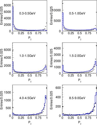
Figure 3: Comparison of the probability distributions of a cluster to be identified as a genuine photon before (histogram) and after (error bars) introducing energy-dependent reference distributions and an improved set of discriminating variables.

Better photon energy calibration is also achieved compared to the previous analysis. The procedure, aiming at a relative calibration between data and simulation, is implemented in several steps. First, a calibration is done using electrons from $\tau$ decays, treating the ECAL information as for a neutral cluster. This method is reliable only above 2 GeV because of the electron track curvature in the magnetic field. Then the final calibration is achieved by comparing the reconstructed $\pi^{0}$ mass and resolution as a function of energy.

Photon conversions are reconstructed following the previous analysis [2].

2.6 $\pi^{0}$ reconstruction

Three different kinds of $\pi^{0}$’s are reconstructed: resolved $\pi^{0}$ from two-photon pairing, unresolved $\pi^{0}$ from merged clusters, and residual $\pi^{0}$ from the remaining single photons after removing radiative, bremsstrahlung and fake photons with a likelihood method.

A $\pi^{0}$ estimator $D_{ij}$ is defined [2], taking into account the photon identification probabilities and the compatibility of the pair with the $\pi^{0}$ mass hypothesis.

As the $\pi^{0}$ energy increases it becomes more difficult to resolve the two photons and the clustering algorithm may yield a single cluster. The two-dimensional energy distribution in the plane perpendicular to the shower direction is examined and energy-weighted moments are computed. Assuming only two photons are present, the second moment provides a measure of the $\gamma\gamma$ invariant mass [11]. Clusters with mass greater than 0.1 GeV/$c^{2}$ are taken as unresolved $\pi^{0}$’s.

After the pairing and the cluster moment analysis, all the remaining photons inside a cone of $30^{\circ}$ around the jet axis are considered. The radiative and bremsstrahlung photons are selected using the same method as described in the previous analysis [2]. Radiative and bremsstrahlung photons are not used in the $\tau$ decay classification discussed below. The behaviour of these estimators was studied in Ref. [2]. The agreement between the number of bremsstrahlung photons in data and simulation is good, but concerns mainly the electron $\tau$ decay channel where this contribution is important (however it does not affect the rate). Bremsstrahlung photons (i.e. radiation along the final state charged pions) in hadronic channels are at a much lower level and they are difficult to pick up unambiguously in the data. To estimate the effect of this contribution one therefore largely relies on the description of radiation at the generator level in the Monte Carlo [16].

2.7 Decay classification

Each $\tau$ decay is classified topologically according to the number of hadronic charged tracks, their particle identification and the number of $\pi^{0}$’s reconstructed. While for 1-prong and 5-prong channels the exact multiplicity is required, the track number in 3-prong channels is allowed to be 2, 3 or 4, in order to reduce systematic effects due to tracking and secondary interactions.

The definition of the leptonic channels requires an identified electron or muon with any number of photons. Some cuts on the total final state invariant mass are introduced to reduce feedthrough from hadronic modes [1].Also some decays with at least two good electron tracks are now included, when one or more of such tracks are classified as converted photons.

In the previous analysis [2], the $3h2\pi^{0}$, $3h3\pi^{0}$ and $h4\pi^{0}$ channels suffered from large backgrounds and consequently had a low signal-to-noise ratio. Most of these backgrounds are due to secondary interactions of the hadronic track with material in the inner detector part. In order to improve the definition of these channels the following steps are taken: (1) require the exact charged multiplicity $n_{ch}=3$ (instead of 2, 3, or 4) for $3h2\pi^{0}$ and $3h3\pi^{0}$, (2) demand a maximum impact parameter of charged tracks less than 0.2 cm (instead of 2 cm) for $3h3\pi^{0}$, and (3) require the number of resolved $\pi^{0}$s in $3h3\pi^{0}$ to be 3 or 2, and 4 or 3 in $h4\pi^{0}$. With these tightened cuts the signal-to-noise ratio improves significantly with a small loss of efficiency.

It should be emphasized that all hemispheres from the selected $\tau\tau$ event sample are classified, except for single tracks going into an ECAL crack (but for identified muons) or with a momentum less than 2 GeV (but for identified electrons and hemispheres with at least one reconstructed $\pi^{0}$). These latter decays, in addition to the rejected ones in the $3h2\pi^{0}$ or $3h3\pi^{0}$ channels are put in a special class, labelled 14, which therefore collects all the non-selected hemispheres. By definition, the sample in class-14 does not correspond to one physical $\tau$ decay mode. In fact, it follows from the simulation that this class comprises about 21% electron, 27% muon, 41% 1-prong hadronic and 11% 3-prong $\tau$ decays. However, consideration of class-14 events can test if the rejected fraction is correctly understood, as discussed later.

The numbers of $\tau$’s classified in each of the considered decay channels are listed in Table 1.

Table 1: Numbers of reconstructed and estimated non-$\tau$ background events in 1991-1993 and 1994-1995 data sets in the different considered topologies.

class	91-93		94-95
$e$	22405	$598\pm 46$	33100	$745\pm 58$
$\mu$	22235	$409\pm 45$	32145	$380\pm 40$
$h$	15126	$93\pm 11$	22429	$100\pm 13$
$h\pi^{0}$	32282	$141\pm 22$	49008	$178\pm 26$
$h2\pi^{0}$	12907	$44\pm 9$	18317	$81\pm 16$
$h3\pi^{0}$	2681	$26\pm 7$	3411	$35\pm 9$
$h4\pi^{0}$	458	$12\pm 3$	499	$19\pm 5$
$3h$	11610	$87\pm 20$	17315	$129\pm 30$
$3h\pi^{0}$	6467	$97\pm 23$	9734	$165\pm 39$
$3h2\pi^{0}$	1091	$27\pm 7$	1460	$36\pm 10$
$3h3\pi^{0}$	124	$13\pm 4$	150	$25\pm 7$
$5h$	60	$3\pm 1$	105	$7\pm 2$
$5h\pi^{0}$	36	$16\pm 5$	59	$21\pm 6$
14	4834	$249\pm 38$	7100	$303\pm 52$
sum	132316	$1815\pm 86$	194832	$2224\pm 107$

The KORAL07 generator [12] in the Monte Carlo simulation incorporates all the decay modes considered in this analysis, except for the $h4\pi^{0}$ decay channel. In the latter case, a separate generation was done where one of the produced $\tau$ is made to decay into that mode using a phase space model for the hadronic final state, while the other $\tau$ was treated with the standard decay library. The complete behaviour between the generated decays and their reconstructed counterparts using the decay classification is embodied in the efficiency matrix. This matrix $\varepsilon_{ji}$ gives the probability of a $\tau$ decay generated in class $j$ to be reconstructed in class $i$. Obtained initially using the simulated samples, it is corrected for effects where data and simulation can possibly differ, such as particle identification, as discussed previously, and photon identification as affected by the presence of fake photons.

2.8 Adjusting the number of fake photons in the simulation

As could be expected, the number of fake photons in the simulation does not agree well with the rate in data. Indeed, it is observed that the rate of low-energy simulated fake photons is insufficient. This effect will affect the classification of the reconstructed final states in the Monte Carlo and bias the efficiency matrix constructed from this sample. A procedure is developed to correct for this effect.

Taking explicitely into account the number $k$ of fake photons in a $\tau$ decay, the efficiency matrix is taken as $\varepsilon_{jik}$, i.e. the efficiency for a produced event in class $j$ with $k$ fake photons reconstructed in class $i$. In this way the effect of the different fake photon multiplicities in data and simulation can be explicitly taken into account, assuming that fake photons are randomly produced. Then, it is sufficient to determine one factor $f_{j}$ in each produced class $j$ in order to quantify the deficit in the simulation. These factors are obtained from fits of the observed $P_{\gamma}$ distributions in data and the number of fake photons produced in the simulation.

In the published analysis using 1991-1993 data [2] a much less sophisticated approach was taken. The deficit of fake photons in the simulation was determined in a global way to be $(16\pm 8)\%$, common to all channels. Since it would have been delicate to generate extra fake photons, the procedure chosen was to actually do the opposite, i.e. randomly kill identified (in the sense of the matching procedure discussed above) fake photons in the simulation, determine the new efficiency matrix and take as corrections the sign-reversed deviations.

It is clear that the current way of dealing with the fake photon problem is both more precise and more reliable. The fact that different channels are treated separately provides a handle on the different origins of the fake photons, since, for example, fake photons in the $h$ class only originate from hadronic interactions, whereas they come from both hadronic interactions and photon shower fluctuations in the $h\pi^{0}$ class.

3 Results

3.1 Determination of the branching ratios

The branching ratios are determined using

$$n^{obs}_{i}-n^{bkg}_{i} = \sum_{j}\varepsilon_{ji}N^{prod}_{j}$$ (1)

$$B_{j} = \frac{N^{prod}_{j}}{\sum_{j}N^{prod}_{j}}$$ (2)

where $n^{obs}_{i}$ is the observed events number in reconstructed class $i$, $n^{bkg}_{i}$ the non-$\tau$ background in reconstructed class $i$, $\varepsilon_{ji}$ the efficiency of a produced class $j$ event reconstructed as class $i$, and $N^{prod}_{j}$ the produced events number of class $j$. The class numbers $i$, $j$ run from 1 to 14, the last one corresponding to the rejected $\tau$ candidates.

The efficiency matrix $\varepsilon_{ji}$ is determined from the Monte Carlo, but corrected using data for many effects such as particle identification efficiency, $\tau\tau$ selection efficiency and fake photon simulation.

The analysis assumes a standard $\tau$ decay description. One could imagine unknown decay modes not included in the simulation, but since large detection efficiencies are achieved in the $\tau\tau$ selection which is therefore robust, these decays would be difficult to pass unnoticed. An independent measurement of the branching ratio for undetected decay modes, using a direct search with a one-sided $\tau$ tag, was done in ALEPH [17], limiting this branching ratio to less than 0.11% at 95% CL. This result justifies the assumption that the sum of the branching ratios for visible $\tau$ decays is equal to one.

The branching ratios are obtained and listed in Table 2.

Table 2: Branching ratios (%) for the reconstructed topologies (quasi-exclusive modes) from 1991-1993 and 1994-1995 data sets; the first error is statistical and the second is systematic.

class	91-93	94-95
$e$	17.859 $\pm$ 0.112 $\pm$ 0.058	17.799 $\pm$ 0.093 $\pm$ 0.045
$\mu$	17.356 $\pm$ 0.107 $\pm$ 0.055	17.273 $\pm$ 0.087 $\pm$ 0.039
$h$	12.238 $\pm$ 0.105 $\pm$ 0.104	12.058 $\pm$ 0.088 $\pm$ 0.083
$h\pi^{0}$	26.132 $\pm$ 0.150 $\pm$ 0.104	26.325 $\pm$ 0.123 $\pm$ 0.090
$h2\pi^{0}$	9.680 $\pm$ 0.139 $\pm$ 0.124	9.663 $\pm$ 0.107 $\pm$ 0.105
$h3\pi^{0}$	1.128 $\pm$ 0.110 $\pm$ 0.086	1.229 $\pm$ 0.089 $\pm$ 0.068
$h4\pi^{0}$	0.227 $\pm$ 0.056 $\pm$ 0.047	0.163 $\pm$ 0.050 $\pm$ 0.040
$3h$	9.931 $\pm$ 0.097 $\pm$ 0.072	9.769 $\pm$ 0.080 $\pm$ 0.059
$3h\pi^{0}$	4.777 $\pm$ 0.093 $\pm$ 0.074	4.965 $\pm$ 0.077 $\pm$ 0.066
$3h2\pi^{0}$	0.517 $\pm$ 0.063 $\pm$ 0.050	0.551 $\pm$ 0.050 $\pm$ 0.038
$3h3\pi^{0}$	0.016 $\pm$ 0.029 $\pm$ 0.020	-0.021 $\pm$ 0.023 $\pm$ 0.019
$5h$	0.098 $\pm$ 0.014 $\pm$ 0.006	0.098 $\pm$ 0.011 $\pm$ 0.004
$5h\pi^{0}$	0.022 $\pm$ 0.010 $\pm$ 0.009	0.028 $\pm$ 0.008 $\pm$ 0.007
14	0.017 $\pm$ 0.043 $\pm$ 0.042	0.099 $\pm$ 0.035 $\pm$ 0.037

3.2 Determination of systematic uncertainties

Wherever possible the efficiencies relevant to the analysis have been determined using ALEPH data, either directly on the $\tau\tau$ sample itself or on specifically selected control samples, as for example in the case of particle identification. The resulting efficiencies are thus measured with known statistical errors.

In some cases the procedure is less straightforward and involves a model for the systematic effect to be evaluated. An important example is given by the systematics in the simulation of fake photons in ECAL. In such cases the evaluation of the systematic error not only takes into account the statistical aspect, but also some estimate of the systematics involved in the assumed model. The latter is obtained from studies where the relevant parameters are varied in a range consistent with the comparison between data and Monte Carlo distributions.

Quite often a specific cut on a given variable can be directly studied. The comparison between the corresponding distributions, respectively in data and Monte Carlo, provides an estimate of a possible discrepancy whose effect would be to change the assumed efficiency of the cut. If a significant deviation is observed, the correction is applied to the simulation to obtain the nominal branching ratio results, while the error on the deviation provides the input to the evaluation of the systematic uncertainty. The analysis is therefore repeated with a full re-classification of all the measured $\tau$ decay candidates, changing the incriminated variable by one standard deviation. Since the new samples slighly differ from the nominal ones because of feedthrough between the different channels, the modified results are affected both by the systematic change in the variable value and the statistical fluctuation from the event sample which is uncommon to both samples. In this case the final systematic uncertainty is obtained by adding linearly the modulus of the systematic deviation observed and the statistical error from the monitored uncommon sample. This procedure is followed for all the systematic studies.

Finally, the systematic deviations for each study are obtained with their sign in each measured decay channel, thus providing the full information on the correlations between the results and allowing the corresponding covariance matrix to be constructed.

The most important systematic uncertainties originate from photon identification and $\pi^{0}$ reconstruction, and secondary interactions.

3.3 From reconstructed classes to exclusive modes

So far branching fractions have been determined in 13 classes corresponding to major $\tau$ decay modes. However, these classes still contain the contributions from final states involving kaons. The latter are coming from Cabibbo-suppressed $\tau$ decays or modes with a $K\overline{K}$ pair, both characterized by small branching ratios compared to the nonstrange modes without kaons. Complete analyses of $\tau$ decays involving neutral or charged kaons have been performed by ALEPH on the full LEP I data [6, 7, 8]. They are summarized and measurements with $K^{0}_{S}$ and $K^{0}_{L}$ are combined in Ref. [9].

The $\tau$ decays involving $\eta$ or $\omega$ mesons also require special attention in this analysis because of their electromagnetic decay modes. Indeed the final state classification relies in part on the $\pi^{0}$ multiplicity, thereby assuming that all photons —but those specifically identified as bremsstrahlung or radiative— originate from $\pi^{0}$ decays. Therefore the non-$\pi^{0}$ photons from $\eta$ and $\omega$ decays are treated as $\pi^{0}$ candidates in the analysis and the systematic bias introduced by this effect must be evaluated. The corrections are based on specific measurements by ALEPH of $\tau$ decay modes containing those mesons [18]. Thus the final results correspond to exclusive branching ratios obtained from the values measured in the topological classification, corrected by the removed contributions from $K$, $\eta$ and $\omega$ modes measured separately, taking into account through the Monte Carlo their specific selection and reconstruction efficiencies to enter the classification. This bookkeeping takes into account all the major decay modes of the considered mesons [19], including the isospin-violating $\omega\rightarrow\pi^{+}\pi^{-}$ decay mode. The main decay modes into consideration are $\pi\omega$, $\pi\pi^{0}\omega$ and $\pi\pi^{0}\eta$ with branching fractions of $(2.26\pm 0.18)~{}10^{-2}$, $(4.3\pm 0.5)~{}10^{-3}$, and $(1.80\pm 0.45)~{}10^{-3}$ [18], respectively. The first two numbers are derived from the branching ratios for the $3\pi\pi^{0}$ and $3\pi 2\pi^{0}$ modes obtained in this analysis and the measured $\omega$ fractions of $0.431\pm 0.033$ from ALEPH [18] and the average value, $0.78\pm 0.06$, from ALEPH [18] and CLEO [20], respectively.

Some much smaller contributions with $\eta$ and $\omega$ have been identified and measured by CLEO [21] with the decay modes $\tau\rightarrow\eta\pi^{-}\pi^{+}\pi^{-}$ ($(2.4\pm 0.5)~{}10^{-4}$), $\tau\rightarrow\eta\pi^{-}2\pi^{0}$ ($(1.5\pm 0.5)~{}10^{-4}$), $\tau\rightarrow\omega\pi^{-}\pi^{+}\pi^{-}$ ($(1.2\pm 0.2)~{}10^{-4}$), and $\tau\rightarrow\omega\pi^{-}2\pi^{0}$ ($(1.5\pm 0.5)~{}10^{-4}$). Even though the corrections from these channels are very small they have been included for the sake of completeness. Finally, another very small correction has been applied to take into account the $a_{1}$ radiative decay into $\pi\gamma$ with a branching fraction of $(2.1\pm 0.8)~{}10^{-3}$ obtained from Ref. [22].

3.4 Overall consistency test

Rejected $\tau$ hemispheres because of charged particle identification cuts (2 GeV minimum momentum and ECAL crack veto for some 1-prong modes, strict definition of higher multiplicity channels) are placed in class 14. As already emphasized, this sample does not correspond to a nominal $\tau$ decay mode and should be explained by all other measured fractions in the other classes and the efficiency matrix. Thus the determination of a hypothetical signal in this class is a measure of the level of consistency achieved in the analysis.

For this determination the efficiency of the possible signal in class 14 is taken to be 100%. The results, already shown in Table 2 separately for the 1991-1993 and 1994-1995 data sets, are consistent and are combined to give $B_{14}=(0.066\pm(0.027)_{stat}\pm(0.021)_{syst,c}\pm(0.025)_{syst,unc})\%$, where the last two errors refer to the common and uncommon uncertainties from the two data sets. With a combined error of $0.042\%$ this value is consistent with zero and provides a good check of the overall procedure at the nontrivial 0.1% level for branching ratios. It is interesting to note that this value coincides, approximately and accidentally, with the limit achieved of 0.11% at 95% CL in a direct search for ’invisible’ decays not selected in the 13-channel classification.

In the following it is assumed that all $\tau$ decay modes have been properly considered at the 0.1% precision level and no physics contribution beyond standard $\tau$ decays is further allowed. Thus the quantity $B_{14}$ is now constrained to be zero.

It can be further noticed that this analysis provides a branching ratio in the $3\pi 3\pi^{0}$ class which is consistent with zero for both 1991-1993 and 1994-1995 data sets (see Table 2). The result is therefore given as an upper limit at 95% CL

$$B_{3\pi 3\pi^{0}}<4.9~{}10^{-4}$$ (3)

consistent with the measurement made by CLEO [23] yielding $B_{3\pi 3\pi^{0}}=(2.2\pm 0.5)~{}10^{-4}$. The final state is dominated by $\eta$ and $\omega$ resonances [23] and using other channels allows one to obtain a lower limit for this branching ratio, $(2.6\pm 0.4)~{}10^{-4}$. In the following a value of $(3\pm 1)~{}10^{-4}$ is used as input for this channel and the global analysis is performed in terms of the remaining 12 defined channels which are refitted.

Figs. 4, 5, 6 and 7 present a few comparisons between data and simulation, providing global checks on the data quality.

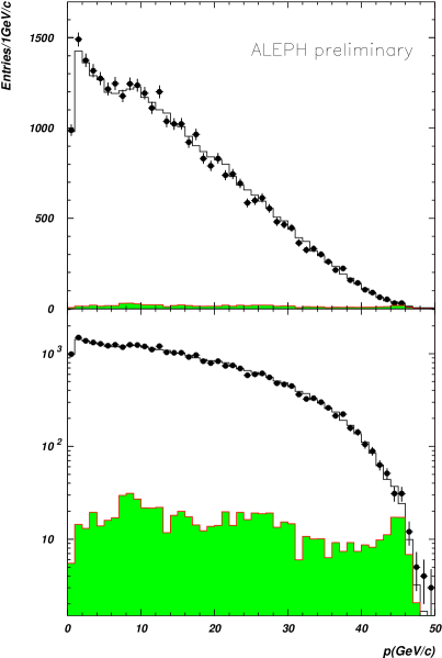
Figure 4: Momentum spectrum in the electron channel in data (error bars) and Monte Carlo (histogram) for the 1994-1995 data set. The shaded histogram is the contribution of non-$\tau$ background.

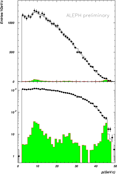
Figure 5: Momentum spectrum in the muon channel in data (error bars) and Monte Carlo (histogram) for the 1994-1995 data set. The shaded histogram is the contribution of non-$\tau$ background.

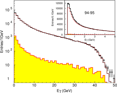
Figure 6: Comparison of photon energy spectra for all $\tau$ events in data (error bars) and Monte Carlo (histogram) after all the corrections for 1994-1995 data set. The dotted line shows the Monte Carlo distribution before correction and the shaded histogram is the contribution of non-$\tau$ background.

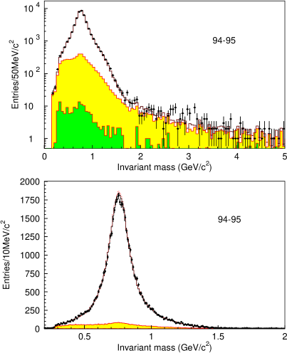
Figure 7: Comparison of mass spectra in data (error bars) and Monte Carlo (histogram) after fake photon correction for the $h\pi^{0}$sample in 1994-1995 data sample. The dark shaded histogram is the contribution of non-$\tau$ background and the light shaded is from $\tau$ feedthrough.

3.5 Comparison of 1991-1993 and 1994-1995 results

Since the same procedure is applied for the analyses of 1991-1993 and 1994-1995 data the results must be consistent within the statistical errors of data and Monte Carlo. Good agreement is observed with a $\chi^{2}$ of 8.6 for 12 DF. In conclusion, the two independent data and Monte Carlo samples give consistent results.

3.6 Final combined results

Finally the two sets of results are combined. Whether one uses only statistical or total weights —in the latter taking into account correlated errors from dynamics and secondary interactions— gives almost identical results. Using the total weights one obtains the final results shown in Table 3.

Table 3: Combined results for the exclusive branching ratios (B) for modes without kaons. The contributions from channels with $\eta$ and $\omega$ are given separately, the latter only for the electromagnetic $\omega$ decays. All results are from this analysis, unless explicitly stated. The values labelled * and **,*** are taken from ALEPH [18] and CLEO [21, 20], respectively.

mode	B $\pm\sigma_{\hbox{stat}}\pm\sigma_{\hbox{syst}}$ [%]
$e$	17.837 $\pm$ 0.072 $\pm$ 0.036
$\mu$	17.319 $\pm$ 0.070 $\pm$ 0.032
$\pi^{-}$	10.828 $\pm$ 0.070 $\pm$ 0.078
$\pi^{-}\pi^{0}$	25.471 $\pm$ 0.097 $\pm$ 0.085
$\pi^{-}2\pi^{0}$	9.239 $\pm$ 0.086 $\pm$ 0.090
$\pi^{-}3\pi^{0}$	0.977 $\pm$ 0.069 $\pm$ 0.058
$\pi^{-}4\pi^{0}$	0.112 $\pm$ 0.037 $\pm$ 0.035
$\pi^{-}\pi^{-}\pi^{+}$	9.041 $\pm$ 0.060 $\pm$ 0.076
$\pi^{-}\pi^{-}\pi^{+}\pi^{0}$	4.590 $\pm$ 0.057 $\pm$ 0.064
$\pi^{-}\pi^{-}\pi^{+}2\pi^{0}$	0.392 $\pm$ 0.030 $\pm$ 0.035
$\pi^{-}\pi^{-}\pi^{+}3\pi^{0}$ (estim.)	0.013 $\pm$ 0.000 $\pm$ 0.010
$3\pi^{-}2\pi^{+}$	0.072 $\pm$ 0.009 $\pm$ 0.012
$3\pi^{-}2\pi^{+}\pi^{0}$	0.014 $\pm$ 0.007 $\pm$ 0.006
$\pi^{-}\pi^{0}\eta^{*}$	0.180 $\pm$ 0.040 $\pm$ 0.020
$\pi^{-}2\pi^{0}\eta^{**}$	0.015 $\pm$ 0.004 $\pm$ 0.003
$\pi^{-}\pi^{-}\pi^{+}\eta^{**}$	0.024 $\pm$ 0.003 $\pm$ 0.004
$a_{1}^{-}(\rightarrow\pi^{-}\gamma)$ (estim.)	0.040 $\pm$ 0.000 $\pm$ 0.020
$\pi^{-}\omega(\rightarrow\pi^{0}\gamma,\pi^{+}\pi^{-})^{*}$	0.253 $\pm$ 0.005 $\pm$ 0.017
$\pi^{-}\pi^{0}\omega(\rightarrow\pi^{0}\gamma,\pi^{+}\pi^{-})^{*,***}$	0.048 $\pm$ 0.006 $\pm$ 0.007
$\pi^{-}2\pi^{0}\omega(\rightarrow\pi^{0}\gamma,\pi^{+}\pi^{-})^{**}$	0.002 $\pm$ 0.001 $\pm$ 0.001
$\pi^{-}\pi^{-}\pi^{+}\omega(\rightarrow\pi^{0}\gamma,\pi^{+}\pi^{-})^{**}$	0.001 $\pm$ 0.001 $\pm$ 0.001

The branching ratios obtained for the different channels are correlated with each other. On one hand the statistical fluctuations in the data and the Monte Carlo sample are driven by the multinomial distribution of the corresponding events, producing well-understood correlations . On the other hand the systematic effects also induce important and nontrivial correlations between the different channels. All the systematic studies were done keeping track of the correlated variations in the final branching ratio results, thus allowing a proper propagation of errors.

The present results are consistent with those of the previously published ALEPH analysis [1, 2]. The leptonic branching ratios also agree within errors with the results of an independent ALEPH analysis which does not rely on a global method [24].

4 Discussion of the results

4.1 Comparison with other experiments

Figs. 8, 9, 10, 11 show that the results of this analysis are in good agreement with those from other most precise experiments. In all these cases, ALEPH achieves the best precision.

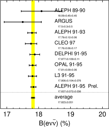
Figure 8: Comparison of ALEPH measurement with published precise results from other experiments for $\tau\rightarrow e\nu\bar{\nu}$.

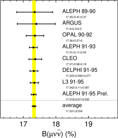
Figure 9: Comparison of ALEPH measurement with published precise results from other experiments for $\tau\rightarrow\mu\nu\bar{\nu}$.

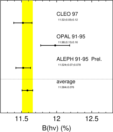
Figure 10: Comparison of ALEPH measurement with published precise results from other experiments for $\tau\rightarrow h\nu$ (sum of $\pi\nu$ and $K\nu$).

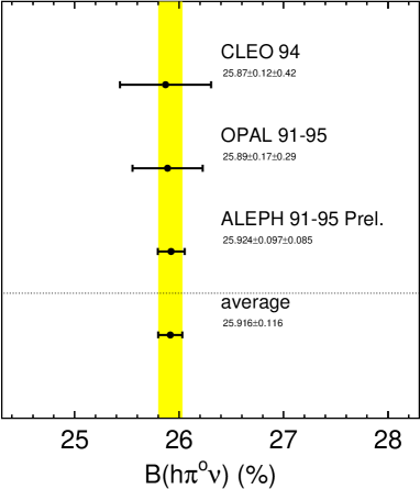
Figure 11: Comparison of ALEPH measurement with published precise results from other experiments for $\tau\rightarrow h\pi^{0}\nu$ (sum of $\pi\pi^{0}\nu$ and $K\pi^{0}\nu$).

A meaningful comparison can be performed between the exclusive fractions and the topological branching ratios. Even though the latter have essentially no physics interest, their determination can constitute a valuable cross check as they depend only on selection efficiency, tracking, handling of secondary interactions and electron identification for photon conversions, and not on photon identification. The results from this analysis can be compared in this way with a dedicated analysis recently performed by DELPHI [25]. Summing up appropriately (both analyses assume a negligible contribution from hadronic multiplicities higher than 5, in agreement with the 90% CL limit by CLEO [26] one gets $B_{7}<2.4~{}10^{-6}$)

$$B_{3} = (14.652\pm 0.067\pm 0.086)~{}\%$$ (4)

$$B_{5} = (0.093\pm 0.009\pm 0.012)~{}\%$$ (5)

in good agreement with the DELPHI values, $B_{3}=(14.569\pm 0.093\pm 0.048)~{}\%$ and $B_{5}=(0.115\pm 0.013\pm 0.006)~{}\%$. The rather small systematic uncertainty in the DELPHI results reflects the fact that a sharper study of hadronic interactions can be performed when only charged particles are considered in the analysis. In addition the modes with $K^{0}_{s}\rightarrow\pi^{+}\pi^{-}$ decays are subtracted statistically here, rather than trying to identify them on an event-by-event basis.

4.2 Universality in the leptonic charged current

4.2.1 $\mu$-e universality from the leptonic branching ratios

In the standard V-A theory with leptonic coupling $g_{l}$ at the $Wl\overline{\nu}_{l}$ vertex, the $\tau$ leptonic partial width can be computed, including radiative corrections [27] and safely neglecting neutrino masses:

$$\Gamma(\tau\rightarrow\nu_{\tau}l\overline{\nu}_{l}(\gamma))=\frac{G_{\tau}G_{l}m^{5}_{\tau}}{192\pi^{3}}f\left(\frac{m^{2}_{l}}{m^{2}_{\tau}}\right)\delta^{\tau}_{W}\delta^{\tau}_{\gamma}~{},$$ (6)

where

$$G_{l} = \frac{g^{2}_{l}}{4\sqrt{2}M^{2}_{W}}$$

$$\delta^{\tau}_{W} = 1+\frac{3}{5}\frac{m^{2}_{\tau}}{M^{2}_{W}}$$

$$\delta^{\tau}_{\gamma} = 1+\frac{\alpha(m_{\tau})}{2\pi}\left(\frac{25}{4}-\pi^{2}\right)$$

$$f(x) = 1-8x+8x^{3}-x^{4}-12x^{2}{\rm ln}x$$ (7)

Numerically, the W propagator correction and the radiative corrections are small: $\delta^{\tau}_{W}=1+2.9\cdot 10^{-4}$ and $\delta^{\tau}_{\gamma}=1+43.2\cdot 10^{-4}$.

Taking the ratio of the two leptonic branching fractions, a direct test of $\mu$-e universality is obtained. The measured ratio

$$\frac{B_{\mu}}{B_{e}}=0.9709\pm 0.0060\pm 0.0029$$ (8)

agrees with the expectation which is equal to 0.97257 when universality holds. Alternatively the measurements yield the ratio of couplings

$$\frac{g_{\mu}}{g_{e}}=0.9991\pm 0.0033$$ (9)

which is consistent with one.

This result is in agreement with the best test of $\mu$-e universality of the W couplings obtained in the comparison of the rates for $\pi\rightarrow\mu\overline{\nu}_{\mu}$ and $\pi\rightarrow e\overline{\nu}_{e}$ decays, where the results of the two most accurate experiments [28, 29] can be averaged to yield $\frac{g_{\mu}}{g_{e}}=1.0012\pm 0.0016$. The results have comparable precision, but it should be pointed out that they are in fact complementary. The $\tau$ result given here probes the coupling to a transverse W (helicity $\pm$1) while the $\pi$ decays measure the coupling to a longitudinal W (helicity 0). It is indeed conceivable that either approach could be sensitive to different nonstandard corrections to universality.

Since $B_{e}$ and $B_{\mu}$ are consistent with $\mu$-e universality their values can be combined, taking common errors into account, into a consistent leptonic branching ratio for a massless lepton (essentially the case for the electron, noting that $f(\frac{m^{2}_{e}}{m^{2}_{\tau}})=1$ for all practical purposes)

$$B^{(m_{l}=0)}_{l}=17.822\pm 0.044\pm 0.022(\%)~{},$$ (10)

where the first error is statistical and the second from systematic effects.

4.2.2 Tests of $\tau$-$\mu$ and $\tau$-e universality

Comparing the rates for $\Gamma(\tau\rightarrow\nu_{\tau}e\overline{\nu}_{e}(\gamma))$, $\Gamma(\tau\rightarrow\nu_{\tau}\mu\overline{\nu}_{\mu}(\gamma))$ and $\Gamma(\mu\rightarrow\nu_{\mu}e\overline{\nu}_{e}(\gamma))$ provides direct tests of the universality of $\tau$-$\mu$-e couplings. Taking the relevant ratios with calculated radiative corrections, one obtains

$$\left(\frac{g_{\tau}}{g_{\mu}}\right)^{2} = \frac{\tau_{\mu}}{\tau_{\tau}}\left(\frac{m_{\mu}}{m_{\tau}}\right)^{5}B_{e}\frac{f(\frac{m^{2}_{e}}{m^{2}_{\mu}})}{f(\frac{m^{2}_{e}}{m^{2}_{\tau}})}\Delta_{W}\Delta_{\gamma}$$ (11)

$$\left(\frac{g_{\tau}}{g_{e}}\right)^{2} = \frac{\tau_{\mu}}{\tau_{\tau}}\left(\frac{m_{\mu}}{m_{\tau}}\right)^{5}B_{\mu}\frac{f(\frac{m^{2}_{e}}{m^{2}_{\mu}})}{f(\frac{m^{2}_{\mu}}{m^{2}_{\tau}})}\Delta_{W}\Delta_{\gamma}$$ (12)

where $f(\frac{m^{2}_{e}}{m^{2}_{\mu}})=0.9998$, $\Delta_{W}=\frac{\delta^{\mu}_{W}}{\delta^{\tau}_{W}}=1-2.9\cdot 10^{-4}$, $\Delta_{\gamma}=\frac{\delta^{\mu}_{\gamma}}{\delta^{\tau}_{\gamma}}=1+8.5\cdot 10^{-5}$, and $\tau_{l}$ is the lepton $l$ lifetime.

From the present measurements of $B_{e}$, $B_{\mu}$, the $\tau$ mass [19], $m_{\tau}=(1777.03^{+0.30}_{-0.26})$ MeV (dominated by the BES result [30]), the $\tau$ lifetime [19], $\tau_{\tau}=(290.6\pm 1.1)$ fs and the other quantities from Ref. [19], universality can be tested:

$$\frac{g_{\tau}}{g_{\mu}} = 1.0009\pm 0.0023\pm 0.0019\pm 0.0004$$ (13)

$$\frac{g_{\tau}}{g_{e}} = 1.0001\pm 0.0022\pm 0.0019\pm 0.0004~{},$$ (14)

where the errors are from the corresponding leptonic branching ratio and the $\tau$ lifetime and mass, respectively.

4.2.3 $\tau$-$\mu$ universality from the pionic branching ratio

The measurement of $B_{\pi}$ also permits an independent test of $\tau$-$\mu$ universality through the relation

$$\left(\frac{g_{\tau}}{g_{\mu}}\right)^{\!\!2} = \frac{B_{\pi}}{B_{\pi\rightarrow\mu\overline{\nu}_{\mu}}}\frac{\tau_{\pi}}{\tau_{\tau}}\frac{2m_{\pi}m_{\mu}^{2}}{m_{\tau}^{3}}$$ (15)

$$\times\;\left(\frac{1-m_{\mu}^{2}/m_{\pi}^{2}}{1-m_{\pi}^{2}/m_{\tau}^{2}}\right)^{\!\!2}\delta_{\tau/\pi}~{},$$

where the radiative correction [31] amounts to $\delta_{\tau/\pi}=1.0016\pm 0.0014$ Using the world-averaged values for the $\tau$ and $\pi$ ($\tau_{\tau}$ and $\tau_{\pi}$) lifetimes, and the branching ratio for the decay $\pi\rightarrow\mu\nu$ [19], the present result for $B_{\pi}$, one obtains

$$\frac{g_{\tau}}{g_{\mu}}=0.9962\pm 0.0048\pm 0.0019\pm 0.0002~{},$$ (16)

comparing the measured value ($B_{\pi}=10.823\pm 0.104$)% to the expected one assuming universality ($10.910\pm 0.042$)%. The quoted errors in Eq. 16 are from the pion mode branching ratio and the $\tau$ lifetime and mass, respectively.

The two determinations of $\frac{g_{\tau}}{g_{\mu}}$ obtained from $B_{e}$ and $B_{\pi}$ are consistent with each other and can be combined to yield

$$\frac{g_{\tau}}{g_{\mu}}=1.0000\pm 0.0021\pm 0.0019\pm 0.0004~{},$$ (17)

where the errors are from the electron and pion branching ratio and the $\tau$ lifetime and mass, respectively. Universality of the $\tau$ and $\mu$ charged-current couplings holds at the 0.29% level with about equal contributions from the present determination of $B_{e}$ and $B_{\pi}$, and the world-averaged value for the $\tau$ lifetime.

The consistency of the present branching ratio measurements with leptonic universality is displayed in Fig. 12 where the result for $B_{e}$ is compared to computed values of $B_{e}$ using as input $B_{\mu}$ (assuming $e-\mu$ universality), $\tau_{\tau}$ and $\tau_{\mu}$ ($\mu-\tau$ universality), and $B_{\pi}$ and $\tau_{\pi}$ ($\mu-\tau$ universality). All values are consistent and yield the average

$$B_{e}^{\rm universality}=(17.810\pm 0.039)~{}\%~{}.$$ (18)

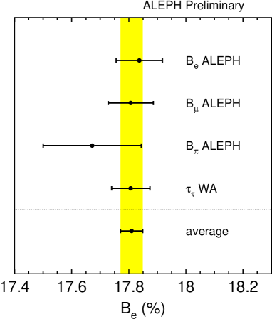
Figure 12: The measured value for $B_{e}$ compared to predictions from other measurements assuming leptonic universality. The vertical band gives the average of all determinations.

4.2.4 $a_{1}$ decays to $3\pi$ and $\pi 2\pi^{0}$

With the level of precision reached it is interesting to compare the rates in the $3\pi$ and $\pi 2\pi^{0}$ channels which are completely dominated by the $a_{1}$ resonance. The dominant $\rho\pi$ intermediate state leads to equal rates, but a small isospin-breaking effect is expected from different charged and neutral $\pi$ masses, slightly favouring the $\pi 2\pi^{0}$ channel.

A recent CLEO partial-wave analysis of the $\pi 2\pi^{0}$ final state [32] has shown that the situation is in fact much more complicated with many intermediate states, in particular involving isoscalars, amounting to about 20% of the total rate and producing strong interference effects. A good description of the $a_{1}$ decays was achieved in the CLEO study, which can be applied to the $3\pi$ final state, predicting [32] a ratio of the rates $3\pi$/$\pi 2\pi^{0}$ equal to 0.985. This value, which includes known isospin-breaking from the pion masses, turns out to be in good agreement with the measured value from this analysis which shows the expected trend

$$\frac{B_{3\pi}}{B_{\pi 2\pi^{0}}}=0.979\pm 0.018~{}.$$ (19)

4.2.5 The $\pi\pi^{0}$ branching ratio in the context of $a_{\mu}^{had}$

The $\pi\pi^{0}$ final state is dominated by the $\rho$ resonance as demonstrated in Fig. 7. Its mass distribution —or better the corresponding spectral function— is a basic ingredient of vacuum polarization calculations, such as that used for computing the hadronic contribution to the anomalous magnetic moment of the muon $a_{\mu}^{had}$. In this case the $\rho$ contribution is dominant (71%) and therefore controls the final precision of the result. The current evaluation [33] used by the BNL experiment [34] is based on $\tau$ and $e^{+}e^{-}$ data, with more precision on the $\tau$ side.

The normalization of the spectral function is provided by the branching fraction $B_{\pi\pi^{0}}$ taken from the world average and completely dominated by the published ALEPH result [2]. The new result given here is larger by 0.68%, thus one can expect a slightly larger contribution to $a_{\mu}^{had}$, but it remains within the quoted uncertainty [33] of $6.2\cdot 10^{-10}$, corresponding to a relative error of 1.2% for the $\rho$ contribution.

A new evaluation [35, 36] is available, using the spectral functions from the present preliminary ALEPH analysis, the published CLEO results [37] and new results from $e^{+}e^{-}$ annihilation from CMD-2 [38]. Since a disagreement is observed between the $\tau$ and $e^{+}e^{-}$ spectral functions, it is important to check all ingredients, in particular the determination of the branching ratio $B_{\pi\pi^{0}}$. As most of the systematic uncertainty in $B_{\pi\pi^{0}}$ comes from $\gamma/\pi^{0}$ reconstruction, it is interesting to cross check the results in the ’adjacent’ hadronic modes, i.e. the $\pi$ and $\pi 2\pi^{0}$ channels. This is possible if universality in the weak charged current is assumed, leading to an absolute prediction of $B_{\pi}$ using as input the $\tau$ lifetime (see Section 4.2.2), and by computing $B_{\pi 2\pi^{0}}$ from the measurement of $B_{3\pi}$ which is essentially uncorrelated with $B_{\pi\pi^{0}}$ (see Section 4.2.4). The comparison, shown in Fig. 13, does not point to any systematic bias in the determination of $B_{\pi\pi^{0}}$ within the quoted uncertainty.

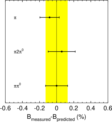
Figure 13: The differences between the measured values for $B_{\pi}$ and $B_{\pi 2\pi^{0}}$ and their respective predictions from leptonic universality and isospin symmetry with $\pi$-mass breaking, compared to the precision on $B_{\pi\pi^{0}}$.

4.2.6 Separation of vector and axial-vector contributions

From the complete analysis of the $\tau$ branching ratios presented in this paper, it is possible to determine the nonstrange vector (V) and axial-vector (A) contributions to the total $\tau$ hadronic width, conveniently expressed in terms of their ratios to the leptonic width, called $R_{\tau,V}$ and $R_{\tau,A}$, respectively. The determination of the strange counterpart $R_{\tau,S}$ is already published [9].

The ratio $R_{\tau}$ for the total hadronic width is calculated from the difference of the ratio of the total hadronic width and electronic branching ratio,

$$R_{\tau} = \frac{1-B_{e}-B_{\mu}}{B_{e}}=\frac{1}{B_{e}}-1.97257$$ (20)

$$= 3.642\pm 0.012~{}.$$

taking for $B(\tau^{-}\rightarrow e^{-}\,\bar{\nu}_{e}\nu_{\tau})$ the value obtained in Section 4.2 assuming universality in the leptonic weak current. Using the ALEPH measurement of the strange width ratio [9], very slightly modified to take into account the channel $K^{*-}\eta$ measured by CLEO [39]

$$R_{\tau,S}=0.1625\pm 0.0066~{},$$ (21)

the following result is obtained for the nonstrange component

$$R_{\tau,V+A}=3.480\,\pm\,0.014~{}.$$ (22)

Separation of V and A components in hadronic final states with only pions is straightforward. Isospin invariance relates the spin-parity of such systems to their number of pions: G-parity =1 (even number) corresponds to vector states, while G=-1 (odd number) tags axial-vector states. This property places a strong requirement on the efficiency of $\pi^{0}$ reconstruction, a constraint that was strongly integrated in this analysis.

Modes with a $K\overline{K}$ pair are not in general eigenstates of G-parity and contribute to both V and A channels. The respective components have been determined in the ALEPH analysis [9]. While the decay to $K^{-}K^{0}$ is pure vector, the $K\overline{K}\pi$ mode has been shown to be almost completely axial vector, with a fraction $0.94^{+0.06}_{-0.08}$. This information was not available at the time of the previous analysis of the nonstrange modes [2] where a conservative value of $0.5\pm 0.5$ was used. For the decays into $K\overline{K}\pi\pi$ no information is available in this respect and the same conservative fraction is assumed.

The total nonstrange vector and axial-vector contributions obtained in this analysis are:

$$R_{\tau,V} = 1.778\pm 0.010\pm 0.002~{},$$ (23)

$$R_{\tau,A} = 1.701\pm 0.011\pm 0.002~{},$$ (24)

where the second errors reflect the uncertainties in the $V/A$ separation in the channels with $K\overline{K}$ pairs. Taking care of the correlations between the respective uncertainties, one obtains the difference between the vector and axial-vector components, which is physically related to the amount of nonperturbative QCD contributions in the nonstrange hadronic $\tau$ decay width:

$$R_{\tau,V-A}=0.077\pm 0.018\pm 0.005~{},$$ (25)

where again the second error has the same meaning as in Eqs. (23) and (24). The ratio

$$\frac{R_{\tau,V-A}}{R_{\tau,V+A}}=0.022\pm 0.005$$ (26)

is a measure of the relative importance of nonperturbative QCD contributions.

5 Conclusions

A final analysis of $\tau$ decay branching fractions using all LEP-I data with the ALEPH detector is presented. As in the publication based on the 1991-1993 data it uses a global analysis of all modes, classified according to charged particle identification, and charged particle and $\pi^{0}$ multiplicity up to 4 $\pi^{0}$s in the final state. Major improvements are introduced with respect to the published analysis and a better understanding is achieved, in particular in the separation between genuine and fake photons. In this process shortcomings and small biases of the previous method were discovered are corrected, leading to more robust results. As modes with kaons ($K^{\pm}$, $K^{0}_{S}$, and $K^{0}_{L}$) have already been studied and published with the full statistics, the nonstrange modes without kaons are emphasized. Taken together these results provide a complete description of $\tau$ decay modes up to 6 hadrons in the final state.

Table 4: A summary list of ALEPH branching ratios (%). The labels $V$, $A$ and $S$ refer to the nonstrange vector and axialvector, and strange components, respectively.

mode	B $\pm\sigma_{\hbox{tot}}$ [%]	(PRELIMINARY!)
$e$	17.837 $\pm$ 0.080
$\mu$	17.319 $\pm$ 0.077
$\pi^{-}$	10.828 $\pm$ 0.105	A
$\pi^{-}\pi^{0}$	25.471 $\pm$ 0.129	V
$\pi^{-}2\pi^{0}$	9.239 $\pm$ 0.124	A
$\pi^{-}3\pi^{0}$	0.977 $\pm$ 0.090	V
$\pi^{-}4\pi^{0}$	0.112 $\pm$ 0.051	A
$\pi^{-}\pi^{-}\pi^{+}$	9.041 $\pm$ 0.097	A
$\pi^{-}\pi^{-}\pi^{+}\pi^{0}$	4.590 $\pm$ 0.086	V
$\pi^{-}\pi^{-}\pi^{+}2\pi^{0}$	0.392 $\pm$ 0.046	A
$\pi^{-}\pi^{-}\pi^{+}3\pi^{0}$	0.013 $\pm$ 0.010	V	estim
$3\pi^{-}2\pi^{+}$	0.072 $\pm$ 0.015	A
$3\pi^{-}2\pi^{+}\pi^{0}$	0.014 $\pm$ 0.009	V
$\pi^{-}\pi^{0}\eta$	0.180 $\pm$ 0.045	V
$(3\pi)^{-}\eta$	0.039 $\pm$ 0.007	A	CLEO
$a_{1}^{-}(\rightarrow\pi^{-}\gamma)$	0.040 $\pm$ 0.020	A	estim
$\pi^{-}\omega(\rightarrow\pi^{0}\gamma,\pi^{+}\pi^{-})$	0.253 $\pm$ 0.018	V
$\pi^{-}\pi^{0}\omega(\rightarrow\pi^{0}\gamma,\pi^{+}\pi^{-})$	0.048 $\pm$ 0.009	A	+ CLEO
$(3\pi)^{-}\omega(\rightarrow\pi^{0}\gamma,\pi^{+}\pi^{-})$	0.003 $\pm$ 0.003	V	CLEO
$K^{-}K^{0}$	0.163 $\pm$ 0.027	V
$K^{-}\pi^{0}K^{0}$	0.145 $\pm$ 0.027	$(94^{+6}_{-8})\%$A
$\pi^{-}K^{0}\overline{K^{0}}$	0.153 $\pm$ 0.035	$(94^{+6}_{-8})\%$A
$K^{-}K^{+}\pi^{-}$	0.163 $\pm$ 0.027	$(94^{+6}_{-8})\%$A
$(K\overline{K}\pi\pi)^{-}$	0.05 $\pm$ 0.02	$(50\pm 50)\%$ A
$K^{-}$	0.696 $\pm$ 0.029	S
$K^{-}\pi^{0}$	0.444 $\pm$ 0.035	S
$\overline{K^{0}}\pi^{-}$	0.917 $\pm$ 0.052	S
$K^{-}2\pi^{0}$	0.056 $\pm$ 0.025	S
$K^{-}\pi^{+}\pi^{-}$	0.214 $\pm$ 0.047	S
$\overline{K^{0}}\pi^{-}\pi^{0}$	0.327 $\pm$ 0.051	S
$(K3\pi)^{-}$	0.076 $\pm$ 0.044	S
$K^{-}\eta$	0.029 $\pm$ 0.014	S

The measured branching ratio values are internally consistent and agree with known constraints from other measurements in the framework of the Standard Model (or even looser assumptions). The precision reached and the completeness of the results are for the moment unique. More specifically, the results on the leptonic and pionic fractions lead to powerful tests of universality in the charged leptonic weak current, showing that the $e-\mu-\tau$ couplings are equal within 2-3 per mille. The branching ratio of $\tau\rightarrow\nu_{\tau}\pi\pi^{0}$ which is of particular interest to the accurate determination of vacuum polarization effects is determined with a precision of 0.5% to be $(25.47\pm 0.13)~{}\%$. Also the ratio of $a_{1}$ branching fractions into $\pi 2\pi^{0}$ and $3\pi$ final states is measured to be $0.979\pm 0.018$, in agreement with expectation from partial wave analyses of these decays. Separating nonstrange hadronic channels into vector (V) and axial-vector (A) components and normalizing to the electronic width yields the ratios $R_{\tau,V}=1.778\pm 0.010$, $R_{\tau,A}=1.701\pm 0.011$, $R_{\tau,V+A}=3.480\pm 0.014$ and $R_{\tau,V-A}=0.077\pm 0.019$.

The results presented here are combined with previously published ALEPH results on final states with kaons in Table 4.

References

- [1] ALEPH Coll., Z. Phys. C70 (1996) 561.
- [2] ALEPH Coll., Z. Phys. C70 (1996) 579.
- [3] ALEPH Coll., Z. Phys. C54 (1992) 211.
- [4] ALEPH Coll., Phys. Lett. B332 (1994) 209.
- [5] ALEPH Coll., Phys. Lett. B332 (1994) 219.
- [6] ALEPH Coll., Eur. Phys. J. C1 (1998) 65.
- [7] ALEPH Coll., Eur. Phys. J. C4 (1998) 29.
- [8] ALEPH Coll., Eur. Phys. J. C10 (1999) 1.
- [9] ALEPH Coll., Eur. Phys. J. C11 (1999) 599.
- [10] ALEPH Coll., Nucl. Instr. Methods A294 (1990) 127.
- [11] ALEPH Coll., Nucl. Instr. Methods, A360 (1995) 481.
- [12] S. Jadach, B.F.L. Ward, and Z. Was, Comp. Phys. Comm. 79 (1994) 503.
- [13] S. Jadach et al., Comp. Phys. Comm. 76 (1993) 361.
- [14] ALEPH Coll., Z. Phys. C62 (1994) 539.
- [15] ALEPH Coll., Eur. Phys. J. C20 (2001) 401.
- [16] E. Barberio, B. van Eijk and Z. Was, Comp. Phys. Comm.66 (1991) 115;E. Barberio and Z. Was, Comp. Phys. Comm.79 (1994) 291.
- [17] S. Snow, Proceedings of the International Workshop on Lepton Physics, Colombus 1992, K. K. Gan ed., World Scientific (1993).
- [18] ALEPH Coll., Z. Phys. C74 (1997) 263.
- [19] Review of Particle Physics, D. E. Groom et al., Eur. Phys. J. C15 (2000) 1.
- [20] D. Bortoletto et al., CLEO Coll., Phys. Rev. Lett. 71 (1993) 1791.
- [21] T. Bergfeld et al., CLEO Coll., Phys. Rev. Lett. 79 (1997) 2406; A. Weinstein, Proceedings of the International Workshop on Lepton Physics, Victoria 2000, R. J. Sobie and J. M. Roney eds., North Holland (2001).
- [22] M. Zielinski et al., Phys. Rev. Lett. 52 (1984) 1195.
- [23] A. Anastassov et al., CLEO Coll., Phys. Rev. Lett. 86 (2001) 4467.
- [24] ALEPH Coll., Proceedings of the Rencontre de Moriond (1999).
- [25] P. Abreu et al., DELPHI Coll., Eur. Phys. J. C20 (2001) 617.
- [26] K. Edwards et al., CLEO Coll., Phys. Rev. D56 (1997) 5297.
- [27] W. Marciano and A. Sirlin, Phys. Rev. Lett. 61 (1988) 1815.
- [28] D.I. Britton et al., Phys. Rev. Lett. 68 (1992) 3000.
- [29] C. Czapek et al., Phys. Rev. Lett. 70 (1993) 17.
- [30] J. Z. Bai et al., Phys. Rev. D53 (1996) 20.
- [31] R. Decker and M. Finkemeier, Phys. Rev. D48 (1993) 4203.
- [32] D. Asner et al., CLEO Coll., Phys. Rev. D61 (2000) 012002.
- [33] M. Davier and A. Höcker, Phys. Lett. B435 (1998) 427.
- [34] G. W. Bennett et al. (Muon (g-2) Collaboration), hep-exp/0208001 (Aug. 2002).
- [35] M. Davier, S. Eidelman, A. Höcker and Z. Zhang, hep-ph/0208177 (Aug. 2002).
- [36] A. Höcker, these proceedings.
- [37] S. Anderson et al. (CLEO Collaboration), Phys.Rev. D61 (2000) 112002.
- [38] R.R. Akhmetshin et al. (CMD-2 Collaboration), Phys.Lett. B527 (2002) 161.
- [39] M. Bishai et al., CLEO Coll., Phys. Rev. Lett. 82 (1999) 281.