Beam Simulation Tools for GEANT4 (and Neutrino Source Applications)

Abstract

Geant4 is a tool kit developed by a collaboration of physicists and computer professionals in the High Energy Physics field for simulation of the passage of particles through matter. The motivation for the development of the Beam Tools is to extend the Geant4 applications to accelerator physics. Although there are many computer programs for beam physics simulations, Geant4 is ideal to model a beam going through material or a system with a beam line integrated to a complex detector. There are many examples in the current international High Energy Physics programs, such as studies related to a future Neutrino Factory, a Linear Collider, and a very Large Hadron Collider.

1 Introduction

Geant4 is a tool kit developed by a collaboration of physicists and computer professionals in the High Energy Physics (HEP) field for simulation of the passage of particles through matter. The motivation for the development of the Beam Tools is to extend the Geant4 applications to accelerator physics. The Beam Tools are a set of C++ classes designed to facilitate the simulation of accelerator elements such as r.f. cavities, magnets, absorbers. These elements are constructed from the standard Geant4 solid volumes such as boxes, tubes, trapezoids, or spheres.

A variety of visualization packages are available within the Geant4 framework to produce an image of the simulated apparatus. The pictures shown in this article were created with Open Inventor [3], which allows direct manipulation of the objects on the screen, plus perspective rendering via the use of light.

Although there are many computer programs for beam physics simulations, Geant4 is ideal to model a beam through a material or to integrate a beam line with a complex detector. There are many such examples in the current international High Energy Physics programs.

2 A Brief Introduction to Geant4

Geant4 is the object oriented C++ version of the Geant3 tool kit for detector simulation developed at CERN. It is currently being used in many fields, such us HEP, space exploration, and medicine.

As a tool kit, Geant4 provides a set of libraries, a main function, and a family of initialization and action classes to be implemented by the user. These classes are singlets, and their associated objects are constructed in main. The objects contain the information related to the geometry of the apparatus, the fields, the beam, and actions taken by the user at different times during the simulation. The Geant4 library classes start with the G4 prefix. The example described in this section, called MuCool, uses only some of the many available user classes.

2.1 Detector and Field Construction

The detector and field geometry, properties, and location are implemented in the constructor and methods of the MuCoolConstruct user class, which inherits from G4VUserDetectorConstruction. In the Construct() method the user does the initialization of the electromagnetic field and the equation of motion. There are a variety of Runge-Kutta steppers to select from, which perform the integration to different levels of accuracy. Next comes the detector description, which involves the construction of solid, logical, and physical volume objects. They contain information about the detector geometry, properties, and position, respectively. Many solid types, or shapes, are available. For example, cubic (box) or cylindric shapes (tube), are constructed as:

G4Box(const G4String& pName, G4double pX, G4double pY, G4double pZ);
G4Tubs(const G4String& pName, G4double pRMin, G4double pRMax,
       G4double pDz, G4double pSPhi, G4double pDPhi);

where a name and half side lengths are provided for the box. Inner, outer radii, half length, and azimuthal coverage are the arguments of a cylinder (tube). A logical volume is constructed from a pointer to a solid, and a given material:

G4LogicalVolume(G4VSolid* pSolid, G4Material* pMaterial,
                const G4String& name)

The physical volume, or placed version of the detector is constructed as:

G4PVPlacement(G4RotationMatrix *pRot, const G4ThreeVector &tlate,
              const G4String& pName, G4LogicalVolume *pLogical,
              G4VPhysicalVolume *pMother, G4bool pMany, G4int pCopyNo);

where the rotation and translation are performed with respect to the center of its “mother” volume (container). Pointers to the associated logical volume, and the copy number complete the list of arguments.

2.2 Physics Processes

Geant4 allows the user to select among a variety of physics processes which may occur during the interaction of the incident particles with the material of the simulated apparatus. There are electromagnetic, hadronic and other interactions available like: “electromagnetic”, “hadronic”, “transportation”, “decay”, “optical”, “photolepton_hadron”, “parameterisation”. The different types of particles and processes are created in the constructor and methods of the MuCoolPhysicsList user class, which inherits from G4VUserPhysicsList.

2.3 Incident Particles

The user constructs incident particles, interaction verteces, or a beam by typing code in the constructor and methods of the MuCoolPrimaryGeneratorAction user class, which inherits from
G4VUserPrimaryGeneratorAction.

2.4 Stepping Actions

The MuCoolSteppingAction user action class inherits from G4UserSteppingAction. It allows to perform actions at the end of each step during the integration of the equation of motion. Actions may include killing a particle under certain conditions, retrieving information for diagnostics, and others.

2.5 Tracking Actions

The MuCoolTrackingAction user action class inherits from G4UserTrackingAction. For example, particles may be killed here based on their dynamic or kinematic properties.

2.6 Event Actions

The MuCoolEventAction user action class inherits from G4UserEventAction. It includes actions performed at the beginning or the end of an event, that is immediately before or after a particle is processed through the simulated apparatus.

3 Description of the Beam Tools Classes

This Section is devoted to explain how to simulate accelerator elements using the Beam Tools. Brief descriptions of each class and constructor are included.

3.1 Solenoids

The Beam Tools provide a set of classes to simulate realistic solenoids. These are BTSheet, BTSolenoid, BTSolenoidLogicVol and BTSolenoidPhysVol.

• The BTSheet class inherits from G4MagneticField. The class objects are field maps produced by an infinitesimally thin solenoidal current sheet. The class data members are all the parameters necessary to generate analytically a magnetic field in $r$-$z$ space (there is $\varphi$ symmetry). No geometric volumes or materials are associated with the BTSheet objects. GetFieldValue is a concrete method of BTSheet inherited from G4Field, through G4MagneticField. It returns the field value at a given point in space and time.

• The BTSolenoid class inherits from G4MagneticField. The class objects are field maps in the form of a grid in $r$-$z$ space, which are generated by a set of BTSheet. The sheets and the BTSpline1D objects, containing the spline fits of $B_{z}$ and $B_{r}$ versus $z$ for each $r$ in the field grid, are data members of BTSolenoid. No geometric volumes or materials are associated with BTSolenoid. The field at a point in space and time is accessed through a GetFieldValue method, which performs a linear interpolation in $r$ of the spline fit objects.

• The BTSolenoidLogicVol class defines the material and physical size of the coil system which is represented by the set of current sheets. A BTSolenoid must first be constructed from a list of current BTSheets. The BTSolenoid object is a data member of BTSolenoidLogicVol. The BTSolenoidLogicVol class constructor creates G4Tubs solid volumes and associated logical volumes for the coil system, the shielding, and the empty cylindric regions inside them. Only the logical volumes are constructed here. No physical placement of a magnet object is done.

• The BTSolenoidPhysVol class is the placed version of the
  BTSolenoidLogicVol. It contains the associated BTSolenoid object as a data member, as well as the pointers to the physical volumes of its logical constituents.

Figure 1 shows a group of four solenoidal copper coil systems modeled with four infinitesimally thin sheets equally spaced in radius.

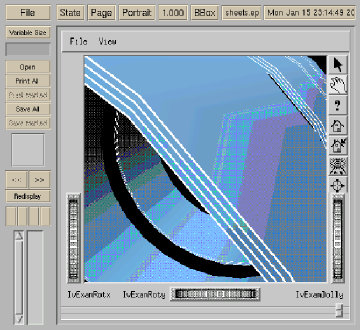
Figure 1: Left: a solenoidal copper coil system modeled with four infinitesimally thin sheets equally spaced in radius. Right: array of four solenoids separated by gaps.

3.2 Magnetic Field Maps

The Beam Tools also allow to simulate generic field maps using the BTMagFieldMap and BTMagFieldMapPlacement classes.

• BTMagFieldMap class inherits from G4MagneticField. The constructor reads the map information from an ASCII file containing the value of the field at a set of nodes of a grid. No geometric objects are associated with the field. The field at a point in space and time is accessed through a GetFieldValue method, as in the case of the solenoid.

• The BTMagFieldMapPlacement class is a placed BTMagFieldMap object. Only the field is placed because there is no coil or support system associated with it.

3.3 r.f. Systems: Pill Box Cavities and Field Maps

This section explains how to simulate realistic r.f. systems using Pill Box cavities. The Beam Tools package provides the classes: BTAccelDevice, BTPillBox, BTrfCavityLogicVol, BTrfWindowLogicVol, and BTLinacPhysVol.

• BTAccelDevice.hh class is abstract. All accelerator device classes are derived from this class, which inherits from G4ElectroMagneticField.

• The BTPillBox class inherits from BTAccelDevice and represents single $\pi/2$ Pill Box field objects. No solid is associated with BTPillBox. The time dependent electric field is computed using a simple Bessel function. It is accessed through a GetFieldValue method. The field is given by:

  $$E_{z}=V_{p}\,J_{0}\left(\frac{2\pi\nu}{c}r\right){\mathrm{s}in}(\phi_{s}+2\pi\nu t)$$ (1)

  $$B_{\mathrm{\varphi}}=\frac{V_{p}}{c}J_{1}\left(\frac{2\pi\nu}{c}r\right){\mathrm{c}os}(\phi_{s}+2\pi\nu t)$$ (2)

  where $V_{p}$ is the cavity peak voltage, $\nu$ the wave frequency, $\phi_{s}$ the synchronous phase, and $J_{0,1}$ the Bessel functions evaluated at $\left(\frac{2\pi\nu}{c}r\right)$.

• The BTrfMap class also inherits from BTAccelDevice. The class objects are electromagnetic field maps which represent an r.f. cavity. In this way, complex r.f. fields can be measured or generated and later included in the simulation. The field map, in the form of a grid, is read in the BTrfMap constructor from an ASCII file. The BTrfMap object is a field, with no associated solid. A GetFieldValue method retrieves the field value at a point in space and time.

• The BTrfCavityLogicVol class constructor creates solid and logical volumes associated with the r.f. field classes. In the case of a map, a vacuum cylinder ring represents its limits. In addition to geometric and material parameters of the cavity, the class contains field and accelerator device information.

• The BTrfWindowLogicVol class is used with BTCavityLogicVol to create the geometry and logical volume of r.f. cavity windows, including the support structure, which may be placed to close the cavity iris at the end cups.

• The BTLinacPhysVol class is a placed linac object. A linac is a set of contiguous r.f. cavities, including the field, the support and conductor material, and windows. The BTLinacPhysVol constructor is overloaded. One version places a linac of Pill Box cavities and the other places field maps.

Fig. 2 shows a Pill Box cavity (in red) with windows. It also shows a cooling channel where solenoids are embedded in large low frequency cavities. Since the beam circulates inside the solenoid, the cavity is represented by a field map (in red) restricted to a cylindric volume with radius slightly smaller than the inner radii of the magnets.

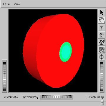
Figure 2: Left: a Pill Box cavity (in red), with windows (green). Right: low frequency cooling channel. The red cylinders are the dummy software structure representing the limits of the electric field maps.

3.4 Tuning the r.f. Cavity Phases

One of the critical elements of an accelerator simulation is the “r.f. tuning”. Each cavity must be operated at the selected synchronous phase at an instant coincident with the passage of the beam. The r.f. wave must be therefore synchronized with the beam, more specifically, with the region of beam phase space that the user needs to manipulate. For this, there is the concept of a reference particle, defined as the particle with velocity equal to the phase velocity of the r.f. wave. If the kinematic and dynamic variables of the reference particle are set to values which are coincident with the mean values of the corresponding variables for the beam, the r.f. system should affect the mean beam properties in a similar way it affects the reference particle.

The Beam Tools allow the use of a “reference particle” to tune the r.f. system before processing the beam. The time instants the particle goes through the phase center of each cavity are calculated and used to adjust each cavity phase to provide the proper kick, at the selected synchronous phase.

3.5 Absorbers

The Beam Tools provide a set of classes to simulate blocks of material in the path of the beam. The constructors create the solid, logical, and physical volumes in a single step. They are all derived from the abstract class of absorber objects BTAbsObj.

• BTCylindricVessel is a system with a central cylindric rim, and two end cup rims with thin windows of radius equal to the inner radius of the vessel. The material is the same for the vessel walls and windows, and the window thickness is constant. The vessel is filled with an absorber material.

• Two classes are available to simulate absorber lenses:
  BTParabolicLense and BTCylindricLense. The first one is a class of parabolic objects with uniform density, and the second a cylinder object with the density decreasing parabolically as a function of radius. From the point of view of the physics effect on the beam, both objects are almost equivalent. The BTParabolicLense is built as a set of short cylinders. The radius is maximum for the central cylinder and reduces symmetrically following a parabolic equation for the others in both sides. The BTCylindricLense object is built from concentric cylinder rings of the same length, different radius, and different densities to mimic a real lens.

The gray cylinder in Fig. 3 is a schematic representation of a liquid hydrogen vessel with aluminum walls and windows. Figure 3 also shows a set of six parabolic lenses in the center of a complex magnetic system. The lenses are placed to mitigate the effect of the decrease in $\langle p_{z}\rangle$ at large radii in a magnetic field flip region, using an emittance exchange mechanism.

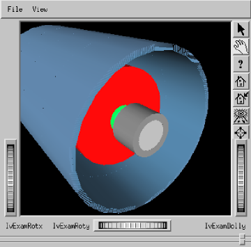
Figure 3: Left: cooling unit cell composed of a solenoid (blue), surrounding the r.f. system (red) and the cylindric absorber vessel (gray). Right: six parabolic lenses (gray) inside a complex magnetic field.

Wedge absorbers are also useful in some cases. They can be easily constructed using the Geant4 trapezoid shape G4Trap.

4 Applications to Neutrino Factory Feasibility Studies

The neutrino beam in a Neutrino Factory would be the product of the decay of a low emittance muon beam. Muons would be the result of pion decay, and pions would be the product of the interaction of an intense proton beam with a carbon or mercury target. Thus the challenge in the design and construction of a Neutrino Source is the muon cooling section, aimed to reduce the transverse phase space by a factor of ten, to a transverse emittance of approximately $\varepsilon_{x}\sim$1 cm.

The ionization cooling technique uses a combination of linacs and light absorbers to reduce the transverse emittance of the beam, while keeping the longitudinal motion under control. There are two competing terms contributing to the change of transverse emittance $\varepsilon_{x}$ along the channel. One is a cooling term, associated with the process of energy loss, and the other is a heating term related to multiple scattering.

4.1 The Double Flip Cooling Channel

The double flip cooling channel is a system consisting of three homogeneous solenoids with two field-flip sections. The first flip occurs at a relatively small magnetic field, B=3 T, to keep the longitudinal motion under control. The field is then increased adiabatically from -3 to -7 T, and a second field flip performed at B=7 T. Figure 4 shows a side view of a lattice unit cell, consisting of a six 201 MHz Pill Box cavities linac and one liquid hydrogen absorber, inside a solenoid. Details on the design and performance of this channel are available in Ref. [6].

4.2 The Helical Channel

The helical channel cools both in the transverse and longitudinal directions. The lattice is based on a long solenoid with the addition of a rotating transverse dipole field, lithium hydride wedge absorbers, and 201 MHz r.f. cavities. Figure 4.4 shows a side view of the helical channel, including the wedge absorbers, idealistic (thin) r.f. cavities, and the trajectory of the reference particle. The design details and performance of this channel are described in Ref. [7].

4.3 The Low Frequency Channel

This is a design based on 44/88 MHz r.f. technology. A unit cell is composed of four solenoids embedded in four r.f. cavities, followed by a liquid hydrogen absorber. Figure 2 shows a unit cell of the low frequency channel, including the solenoids, the absorber, and the relevant section of the r.f. field map (inside the magnets). More information about this channel may be found in Ref. [5].

4.4 Other Systems

Among other simulations performed with the Beam Tools for Geant4 we may cite: the Alternate Solenoid Channel (sFoFo) [8], and a High Frequency Buncher/Phase Rotator scheme for the neutrino factory [9, 10].

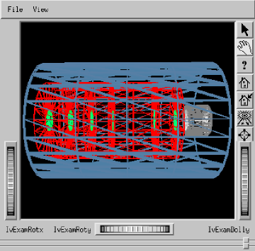
Figure 4: Left: side view of the double flip channel unit cell, including the solenoid, the six Pill Box cavities, and the absorber. Right: image of the helical channel, including the wedge absorbers (yellow and green), idealistic thin r.f. cavities (blue), and the trajectory of the reference particle (red).

5 Summary

The Beam Physics Tools for Geant4 are used in numerous accelerator studies, reported in conference proceedings and proposals. Geant4 is especially suited to systems where accelerators, shielding, and detectors must be studied jointly with a simulation. The Beam Tool libraries, a software reference manual, and a user’s guide, are available from the Fermilab Geant4 web page [11].

References

- [1] See Geant4 home page at: wwwinfo.cern.ch/asd/geant4/geant4.html.
- [2] See Root home page at: http://root.cern.ch/root.
- [3] Open Inventor. Registered trademark of Silicon Graphics Inc.
-
[4]
See ZOOM home page at:
http://www.fnal.gov/docs/working-groups/fpcltf/Pkg/WebPages/zoom.html. -
[5]
“Pseudo-Realistic GEANT4 Simulation of a 44/88 MHz Cooling Channel for the Neutrino Factory”, V. D. Elvira, H. Li, P. Spentzouris.
MuCool note 230, 12/10/01.
http://www-mucool.fnal.gov/notes/noteSelMin.html - [6] “The Double Flip Cooling Channel”, V. Balbekov, V. Daniel Elvira et al. Published in PAC2001 proceedings, Fermilab-Conf-01-181-T.
- [7] “Simulation of a Helical Channel Using GEANT4”, V. D. Elvira et al. Published in PAC2001 proceedings, Fermilab-Conf-01-182-T.
- [8] “Feasibility Study 2 of a Muon Based Neutrino Source”, S. Ozaki et al. BNL-52623, Jun 2001.
-
[9]
“High Frequency Adiabatic Buncher ”, V. Daniel Elvira,
MuCool note 253, 8/30/02.
http://www-mucool.fnal.gov/notes/noteSelMin.html -
[10]
“Fixed Frequency Phase Rotator for the Neutrino Factory”,
N. Keuss and V. D. Elvira,
MuCool note 254, 8/30/02.
http://www-mucool.fnal.gov/notes/noteSelMin.html - [11] See Fermilab Geant4 web page at: http://www-cpd.fnal.gov/geant4.