CLEO Contributions to Tau Physics

Abstract

We review many of the contributions of the CLEO experiment to tau physics. Topics discussed are: branching fractions for major decay modes and tests of lepton universality; rare decays; forbidden decays; Michel parameters and spin physics; hadronic sub-structure and resonance parameters; the tau mass, tau lifetime, and tau neutrino mass; searches for CP violation in tau decay; tau pair production, dipole moments, and CP violating EDM; and tau physics at CLEO-III and at CLEO-c.

1 Introduction

Over the last dozen years, the CLEO Collaboration has made use of data collected by the the CLEO-II detector [2] to measure many of the properties of the tau lepton and its neutrino. Now that the experiment is making a transition from operation in the 10 GeV (B factory) region to the 3-5 GeV tau-charm factory region [3], it seemed to the author and the Tau02 conference organizers to be a good time to review the contributions of the CLEO experiment to tau physics. We are consciously omitting results from CLEO-I (data taken before 1989). The author has chosen to take a semi-critical approach, emphasizing both the strengths and weaknesses of tau physics at CLEO: past, present, and future.

2 Tau Production at 10 GeV

We begin by discussing a topic on which CLEO has not published: tau pair production.

In $e^{+}e^{-}$ collisions, one can study taus in production and/or decay. The production reaction $e^{+}e^{-}\to\gamma^{*}\to\tau^{+}\tau^{-}$ is governed by well-understood QED. As such, it is not terribly interesting (or at least, nowhere near as interesting as studying $e^{+}e^{-}\to\gamma^{*}/Z^{(*)}\to\tau^{+}\tau^{-}$ at LEP I and LEP II). CLEO has studied resonance production and decay, e.g., in [4] $e^{+}e^{-}\to\Upsilon(nS)\to\tau^{+}\tau^{-}$.

In addition to overall rate, one can search for small anomalous couplings. Rather generally, these can be parameterized as anomalous magnetic, and (CP violating) electric, dipole moments. With $\tau^{+}\tau^{-}$ final states, one can study the spin structure of the final state; this is perhaps the most sensitive way to search for anomalous couplings. We will return to this subject in section 9.1.

Measuring the production rate at 10 GeV is only interesting if it is precise: $<1\%$. This has proven to be difficult at CLEO, for several reasons.

First, it is desirable to do an inclusive selection of $\tau^{+}\tau^{-}$ final states, so that production rates don’t depend on decay branching fractions, which were not measured at the 1% level in the early part of the last decade. It’s difficult to select taus inclusively, because backgrounds from $q\bar{q}$, $e^{+}e^{-}$, $\mu^{+}\mu^{-}$ and two-photon are less easily distinguishable from $\tau^{+}\tau^{-}$ than at LEP, and they depend on tau decay mode. It’s not really hard, but it’s hard to get precise selection efficiencies. In the end, tau selection at CLEO always had smaller efficiencies and/or larger backgrounds, and often also larger systematic errors, than analogous analyses at LEP.

To measure the production cross-section, one needs a precise luminosity measurement, with an error $<<1\%$. At CLEO, we selected large angle Bhabhas ($e^{+}e^{-}$), $\mu^{+}\mu^{-}$, $e^{+}e^{-}\to\gamma\gamma$ with rather high statistics. To get the luminosity, we need accurate predictions of the cross-section times selection efficiency from precision Monte Carlo simulations, incorporating accurate QED radiative corrections. Much less effort has gone into this at 10 GeV than at LEP! Each of these measurements has small statistical errors, but the systematic errors are of the order of $\sim 2\%$. CLEO got agreement between the 3 QED processes at the level of 1% but not much better; the discrepancies are likely to be in the QED Monte Carlos. CLEO quotes a 1% systematic error on luminosity [5].

The moral is that further progress in this topic requires precision QED Monte Carlos. The KKMC program [6] promises precision results, but it must be validated with careful computational and experimental cross-checks. Consistent results for $e^{+}e^{-}$, $\mu^{+}\mu^{-}$, $e^{+}e^{-}\to\gamma\gamma$ are a good first step. Further, measurements of anomalous moments make use of the spin correlations in tau pair production at 10 GeV, so one must validate the correct treatment of spin-dependence in the Monte Carlo.

3 Tau decay physics at CLEO

CLEO pursued a systematic study of all tau decays during the 1990’s, learning much about the tau, its neutrino, and low-energy meson dynamics. The main decay modes are listed in Table 1.

Table 1: Main decay modes of the $\tau$ lepton.

$\tau\rightarrow e\nu\nu_{\tau}$	$\approx 18\%$	Br, univ, Michel
$\tau\rightarrow\mu\nu\nu_{\tau}$	$\approx 17\%$	Br, univ, Michel
$\tau\rightarrow\pi\nu,\,K\nu_{\tau}$	$\approx 12\%$	Br, univ
$\tau\rightarrow\pi\pi\nu_{\tau}$	$\approx 25\%$	Br, $\rho$, $\rho^{\prime}$, CVC, $\Pi$
$\tau\rightarrow K\pi\nu_{\tau}$	$\approx 1.4\%$	Br, $K^{*}$, $K^{*\prime}$
$\tau\rightarrow 3\pi\nu_{\tau}$	$\approx 18\%$	Br, $a_{1}$, $a_{1}^{\prime}$, $h_{\nu_{\tau}}$
$\tau\rightarrow K\pi\pi\nu_{\tau}$	$\approx 0.8\%$	Br, $K_{1}$, $K_{1b}$, W-Z
$\tau\rightarrow 4\pi\nu_{\tau}$	$\approx 5\%$	Br, $\rho^{\prime}$, CVC
$\tau\rightarrow\mbox{rare}$	$\approx 2\%$	$5\pi$, $6\pi$, $\eta\pi\pi$, …
$\tau\to\eta\pi\nu,b_{1}\nu_{\tau}$	$\ll 1\%$	2nd-class currents
$\tau\rightarrow\mbox{forbidden}$	$\ll 1\%$	neutrinoless decays

3.1 One-prong problem

In the early 90’s, the “tau one-prong” problem was raging; the branching fractions for exclusively reconstructed tau decays didn’t add up to 1 [7]. The resolution of this discrepancy required precision (sub-1%) branching fractions measurements.

CLEO-II was a new detector; acceptances, in/efficiencies, and detector simulation needed to be understood very well. Important issues included the detection of $\pi^{0}$’s: they rarely merged into one shower, and CLEO obtained great $m_{\gamma\gamma}$ resolution ($\sim$ 6 MeV) with its CsI calorimeter. However, soft photons could get lost; and “splitoffs” from hadronic showers could fake photons. Overall, ensuring reliable detection of $\pi^{0}$’s resulted in a detection efficiency $\sim 50(1\pm 0.03)\%$. Also, CLEO had poor K/$\pi$ separation over most of the interesting momentum range. We made progress using $K^{0}_{S}$, with detection efficiency $\sim 50\%$. Because of all this, it was hard to know the overall detection efficiency, after backgrounds, to better than 1%.

Ultimately, CLEO’s branching fraction measurements were limited by knowledge of luminosity (1%), cross-section (computed to order $\alpha$ with KORALB [8], $\sim 1\%$), and knowledge of the detection efficiency and backgrounds ($\sim 1-2\%$). However, with millions of produced $\tau^{+}\tau^{-}$, what we lacked in efficiency we made up for in statistics.

By 1995, we made $\sim(1-2)\%$ measurements of branching fractions to $e\nu\nu_{\tau}$, $\mu\nu\nu_{\tau}$, $\pi/K\nu_{\tau}$, $\pi\pi^{0}\nu_{\tau}$, $\pi n\pi^{0}\nu_{\tau}$, $3\pi\nu_{\tau}$, $3\pi\pi^{0}\nu_{\tau}$, etc.[9, 10, 11, 12]. These measurements reduced the “tau one-prong” problem to insignificance by PDG 1996 [13]. We had also tested $e/\mu/\tau$ charged-current coupling universality at the 1% level [9]. By then, LEP was measuring branching fractions with total errors much smaller than $1\%$. This came as quite a shock to CLEO! It helped that the LEP experiments knew $N_{\tau\tau}=\sigma{\cal L}$ quite well, as a by-product of their incredibly successful electroweak program.

4 Rare semi-hadronic decay modes

Rare semi-hadronic decay modes of the tau provide unique laboratories for low-energy meson dynamics, and tests of conservation laws. With the world’s largest sample of tau pairs throughout the 1990’s, CLEO made many first and/or most precise measurements of rare decay modes [14, 15, 16, 17, 18], listed in Table 2.

Table 2: Measurements of branching fractions for rare semi-hadronic $\tau$ decay modes by CLEO-II.

$${\cal B}(2\pi^{-}\pi^{+}2\pi^{0}\nu_{\tau}) =(5.3\pm 0.4)\times 10^{-3}$$

$${\cal B}(3\pi^{-}2\pi^{+}\nu_{\tau}) =(7.8\pm 0.6)\times 10^{-4}$$

$${\cal B}(2\pi^{-}\pi^{+}3\pi^{0}\nu_{\tau}) =(2.2\pm 0.5)\times 10^{-4}$$

$${\cal B}(3\pi^{-}2\pi^{+}\pi^{0}\nu_{\tau}) =(1.7\pm 0.3)\times 10^{-4}$$

$${\cal B}(\pi^{-}2\pi^{0}\omega\nu_{\tau}) =(1.5\pm 0.5)\times 10^{-4}$$

$${\cal B}(2\pi^{-}\pi^{+}\omega\nu_{\tau}) =(1.2\pm 0.3)\times 10^{-4}$$

$${\cal B}(3\pi^{-}2\pi^{+}2\pi^{0}\nu_{\tau}) <1.1\times 10^{-4}$$

$${\cal B}(7\pi^{\pm}(\pi^{0})\nu_{\tau}) <2.4\times 10^{-6}.$$

Decay modes like $5\pi$, $6\pi$, $7\pi$, $\eta\pi\pi$, $\eta 3\pi$, are relatively easy to reconstruct. The big problem is background from $q\bar{q}$. Lepton tags can clean that up reasonably well, but an irreducible background remains, that can be estimated and subtracted statistically. These modes have rich and complicated sub-structure, which we attempted to delve into for the $5\pi$, $6\pi$, and $\eta 3\pi$ modes. Some $6\pi$ signals are shown in Fig. 1.

Of particular interest are modes involving $\eta$ mesons [19, 20, 21, 22], listed in Table 3.

Table 3: Measurements of $\tau$ decay modes involving kaons from CLEO-II.

$${\cal B}(\nu_{\tau}\eta\pi^{-}) < 1.4\times 10^{-4}\mbox{at 95\%\ CL}$$

$${\cal B}(\nu_{\tau}\eta K^{-}) = (2.6\pm 0.5)\times 10^{-4}$$

$${\cal B}(\nu_{\tau}\eta\pi^{-}\pi^{0}) = (1.7\pm 0.3)\times 10^{-3}$$

$${\cal B}(\nu_{\tau}\eta\pi^{-}\pi^{+}\pi^{-}) = (3.4\pm 0.8)\times 10^{-4}$$

$${\cal B}(\nu_{\tau}\eta\pi^{-}\pi^{0}\pi^{0}) = (1.4\pm 0.6)\times 10^{-4}$$

$${\cal B}(\nu_{\tau}K^{*-}\eta) = (2.90\pm 0.80\pm 0.42)\times 10^{-4}.$$

The $\eta\pi^{-}$ mode is a signature for second-class (isospin-violating) currents. The $\eta K^{-}$ mode proceeds by SU(3)_f violation. The $\eta\pi^{-}\pi^{0}$ mode proceeds by the Wess-Zumino anomalous current. The $\eta 3\pi$ signals, which are rich in sub-structure, are shown in Fig. 2.

CLEO also observed the radiative decay modes $\tau^{-}\to e^{-}\nu_{\tau}\gamma$ and $\tau^{-}\to\mu^{-}\nu_{\tau}\gamma$ [23], and made the first observation of the decays $\tau^{-}\to e^{-}e^{+}e^{-}\bar{\nu}_{e}\nu_{\tau}$ (5 events) and $\tau^{-}\to\mu^{-}e^{+}e^{-}\bar{\nu}_{\mu}\nu_{\tau}$ (1 event) [24].

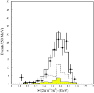
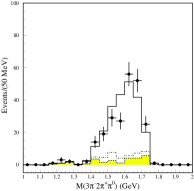
Figure 1: Mass distributions from $\tau\to 6\pi\nu_{\tau}$. The data are shown as data points with error bars, the lower histograms show various background models, and the open solid histogram shows the model of the background plus tau decay signal. Left: $M(2\pi^{-}\pi^{+}3\pi^{0}\nu_{\tau})$ in $\tau^{-}\to 2\pi^{-}\pi^{+}3\pi^{0}\nu_{\tau}$ [16]. Right: $M(3\pi^{-}2\pi^{+}\pi^{0})$ in $\tau^{-}\to 3\pi^{-}2\pi^{+}\pi^{0}\nu_{\tau}$ [17].

Figure 2: Mass distributions from $\tau\to 3\pi\eta\nu_{\tau}$ [21]. The data are shown as data points with error bars, the hatched histogram shows the background model (mostly from non-tau continuum), and the open solid histogram shows the model of the background plus tau decay signal. $M((3\pi)^{-}\eta)$ is plotted, for (a) $2\pi^{-}\pi^{+}\eta$, $\eta\to\gamma\gamma$; (b) $2\pi^{-}\pi^{+}\eta$, $\eta\to 3\pi^{0}$; (c) $\pi^{-}2\pi^{0}\eta$, $\eta\to\gamma\gamma$.

4.1 Rare strange modes - $X_{S}^{-}\nu_{\tau}$

Modes with $K^{0}_{S}$ are easily accessible in the CLEO data. Identifying charged kaons was problematical in CLEO-II, but even with poor K/$\pi$ separation ($\sim<2\sigma$), we identified and measured branching fractions for many modes containing kaons, listed in Table 4. During the same time period, LEP-I produced terrific results on modes with kaons, including $K^{0}_{L}$!

Table 4: Measurements of $\tau$ decay modes involving kaons from CLEO-II.

${\cal B}(\bar{K^{0}}\pi^{-}\pi^{0}\nu_{\tau})$	= ($0.417\pm 0.058\pm 0.044$)%
${\cal B}(K^{-}\pi^{+}\pi^{-}\nu_{\tau})$	= ($0.345\pm 0.023\pm 0.055$)%
${\cal B}(K^{-}\pi^{0}\pi^{0}\nu_{\tau})$	= ($0.14\pm 0.10\pm 0.03$)%
${\cal B}(K^{-}K^{0}\pi^{0}\nu_{\tau})$	= ($0.145\pm 0.036\pm 0.020$ )%
${\cal B}(K^{-}K^{+}\pi^{-}\nu_{\tau})$	= ($0.144\pm 0.013\pm 0.028$ )%
${\cal B}(K^{0}_{S}K^{0}_{S}\pi^{-}\nu_{\tau})$	= ($0.023\pm 0.005\pm 0.003$ )%
${\cal B}(K^{-}\pi^{+}\pi^{-}\pi^{0}\nu_{\tau})$	= ($0.075\pm 0.026\pm 0.017$)%
${\cal B}(K^{-}K^{+}\pi^{-}\pi^{0}\nu_{\tau})$	= ($0.033\pm 0.018\pm 0.007$)%

5 Forbidden (neutrinoless) decays

Tau decays to final states with no $\nu_{\tau}$ (or more precisely, no missing energy) are a clear signature for lepton-number violation, pointing directly to physics beyond the Standard Model. The golden mode is $\tau\to\mu\gamma$, which in many models, would be the easiest to observe in tau decays (despite the strong constraint from non-observation of $\mu\to e\gamma$).

CLEO-II set its first upper limit ${\cal B}(\tau\to\mu\gamma)<4.2\times 10^{-6}$ (90% CL) in 1992 [25]. This was improved to $3.0\times 10^{-6}$ by 1996 ($4.3\times 10^{6}$ tau pairs) [26]; then $1.1\times 10^{-6}$ by 1999 ($12.6\times 10^{6}$ tau pairs) [27]. By this point, we were starting to hit background events (see Fig. 3), which appear to be irreducible; further progress can no longer be expected to scale inversely with the number of produced tau pairs.

CLEO also searched for many other neutrinoless modes, setting limits on 22 of them in 1994 [28], with branching fraction upper limits around $10^{-5}$. This was updated in 1997 [29], with 28 modes, including resonances; branching fraction upper limits of a few $\times 10^{-6}$ were obtained. We added 10 more modes with $\pi^{0}$’s and/or $\eta$’s in 1997 [30]. Five more modes were added in 1998 [31], containing (anti-)protons: $\tau^{-}\to\bar{p}X^{0}$.

Throughout all this, we managed to forget about modes containing $K^{0}$’s! This has now been corrected: New for this conference [32], based on $12.7\times 10^{6}$ $\tau^{+}\tau^{-}$), are the branching fraction upper limits at 90% CL listed in Table 5.

Table 5: Measurements of neutrinoless $\tau$ decay modes involving $K^{0}_{S}$’s, from CLEO-II [32].

$${\cal B}(e^{-}K^{0}_{S}) < 9.1\times 10^{-7}$$

$${\cal B}(\mu^{-}K^{0}_{S}) < 9.5\times 10^{-7}$$

$${\cal B}(e^{-}K^{0}_{S}K^{0}_{S}) < 2.2\times 10^{-6}$$

$${\cal B}(\mu^{-}K^{0}_{S}K^{0}_{S}) < 3.4\times 10^{-6}$$

Figure 3: CLEO data (points) and Monte Carlo prediction (open boxes) for $\tau^{-}\to\mu^{-}\gamma$ [27].

6 CLEO Michel Parameter analyses

We turn now from measurements of branching fractions to the substructure in the multi-particle decay modes. For the leptonic decays $\tau^{-}\to\ell^{-}\bar{\nu}_{\ell}\nu_{\tau}$, this amounts to the measurement of the Michel parameters governing the Lorentz structure of the decay (i.e., the search for deviations from the Standard Model $V-A$ structure). Information on the Lorentz structure of the decay, especially on the helicity of the tau neutrino $h_{\nu_{\tau}}$, can also be obtained from decay distributions in semi-hadronic ($\tau^{-}\to X_{h}^{-}\nu_{\tau}$) decays.

CLEO-II has published four different analyses focusing on Lorentz structure:

• Select $\ell^{-}\overline{\nu}{\nu_{\tau}}$ vs. $\pi^{+}\mbox{$\pi^{0}\,$}{\overline{\nu}}_{\tau}$; Use $\pi^{\pm}\pi^{0}$ as tag. From the lepton energy spectrum, extract the Michel parameters $\rho$ and $\eta$ [33].

• Select $\pi^{-}{\nu_{\tau}}$ vs. $\pi^{+}{\overline{\nu}}_{\tau}$; exploit the spin correlations between the two taus in the event to extract the square of the tau neutrino helicity $|h_{\nu_{\tau}}|^{2}$ [34].

• Select $\ell^{-}\overline{\nu}{\nu_{\tau}}$ vs. $\pi^{+}\mbox{$\pi^{0}\,$}{\overline{\nu}}_{\tau}$; use the $\pi^{\pm}\pi^{0}$ decay as spin analyzer. Use the full event kinematics to extract measurements of the Michel parameters $\rho$, $\eta$, $\xi$, $\delta$, and $|h_{\nu_{\tau}}|$ [35].

• Select $\ell^{-}\overline{\nu}{\nu_{\tau}}$ vs. $(\rho\pi)^{-}{\overline{\nu}}_{\tau}$. Exploit the interference between the two $\rho\pi$ amplitudes, and use the full event kinematics to extract the parity-violating signed tau neutrino helicity $h_{\nu_{\tau}}$ [36].

The third-listed analysis [35], in particular, made rather precise measurements, using a powerful technique. To make full use of kinematical information, a full multi-dimensional likelihood fit was performed. The fit correlated information on the $\rho^{+}$ polarization in $\tau^{+}\to\rho^{+}\nu_{\tau}$ from the decay $\rho^{+}\to\pi^{+}\pi^{0}$, the QED-predicted correlations between the spins of the $\tau^{+}$ and the $\tau^{-}$, and the momentum distribution of the daughter lepton in $\tau^{-}\to\ell^{-}\overline{\nu}{\nu_{\tau}}$, in order to extract the spin-independent Michel parameters $\rho$ and $\eta$, the spin-dependent parameters $\xi$ and $\xi\delta$, and the tau neutrino helicity $h_{\nu_{\tau}}$. This is illustrated in Fig. 4.

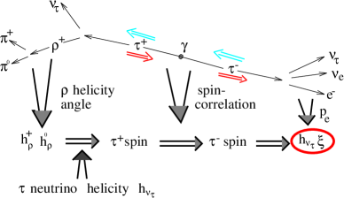
Figure 4: Illustration of how to extract spin-dependent Michel parameters in the reaction $e^{+}e^{-}\to\tau^{+}\tau^{-}$, $\tau^{+}\to\rho^{+}\nu_{\tau}$, $\tau^{-}\to\ell^{-}\overline{\nu}{\nu_{\tau}}$.

The Michel parameters measured in this way are compared with those from other experiments in Fig. 5. From these measurements, strong constraints could be placed on right-handed $\tau-\nu_{\tau}$ couplings and the mass of a right-handed $W^{\pm}_{R}$. Further, the precise limit obtained on $\eta$ (without making use of any constraint on $\eta$ from the leptonic branching fractions) sets a constraint on the presence of, e.g., a scalar charged Higgs mediating tau decays.

Figure 5: Measurements of tau Michel parameters from CLEO’97 and from other experiments. ^∗The leptonic branching fractions were used to further constrain the value of $\eta$ in the OPAL 98 measurement.

7 Hadronic substructure in tau decays

Tau semi-hadronic decays $\tau^{-}\to X_{h}^{-}\nu_{\tau}$ provide a uniquely clean probe of low energy meson dynamics. Recall that strong dynamics is the most poorly understood part of the Standard Model. The fundamental theory is QCD, but it is difficult to use QCD to characterize hadronic structure in detail. Instead, we must rely on models, symmetries and conservation laws (such as isospin and $SU(3)_{f}$), the Conserved Vector Current (CVC) hypothesis, sum rules, chiral perturbation theory, and results from QCD on the lattice.

The momentum transfer is small in $\tau$ decays; we are in the region where resonances dominate, and their description relies on phenomenological models. The dynamics of such hadronic systems is parameterized in tau decays via the “spectral function” $v(q^{2})$ ($q^{2}=M(X_{h})^{2}$), containing all the strong dynamics. These spectral functions can be related, via CVC, to similar quantities in $e^{+}e^{-}$ collisions and in vacuum polarization diagrams that arise in $(g-2)_{\mu}$ and $\alpha(q^{2})$ [37]. CLEO can measure $v(q^{2})$ using exclusive final states; it is more problematic to do inclusive studies such as has been done at LEP, as discussed above. Still, CLEO published one paper on the subject [38], extracting $\alpha_{S}(m^{2}_{\tau})$.

CLEO has studied substructure in the following tau decays:

• $\tau^{-}\to\pi^{-}\pi^{0}\nu_{\tau}$ [39]; see Fig. 6. We extracted the mass and width of the $\rho^{-}$ meson and the mass, width, and coupling of the $\rho^{\prime-}$ meson; measured the pion form factor $|F_{\pi}(q^{2})|$; and provided tests of CVC in comparison with $e^{+}e^{-}\to\pi^{+}\pi^{-}$ (see [40]). These data are useful in the evaluation of the hadronic contribution to the vacuum polarization diagrams that arise in $(g-2)_{\mu}$ and $\alpha(q^{2})$ [37].

• $\tau^{-}\to\pi^{-}K^{0}\nu_{\tau}$ [41], see Fig. 7. We studied the mass and width of $K^{*-}$ meson, looked for evidence of a $K^{*\prime-}$, and extracted the decay constant $f_{K^{*}}$. This work has not yet been published! Of particular note is a significant discrepancy between the mass of the $K^{*-}$ seen in our clean sample from $\tau^{-}\to K^{*-}\nu_{\tau}$ and the world average in the PDG.

• $\tau^{-}\to 3\pi\nu_{\tau}$; see Fig. 6. We have performed three analyses: a model-dependent analysis using the $\pi^{-}\pi^{0}\pi^{0}$ mode [36], a model-independent measurement of the structure functions using the $\pi^{-}\pi^{0}\pi^{0}$ mode [42], and a model-dependent analysis using the $\pi^{-}\pi^{+}\pi^{-}$ mode [43]. We found a rich structure, including the presence of scalar and tensor mesons. We measured the decay constant $f_{a_{1}}$; the signed neutrino helicity $h_{\nu_{\tau}}$; and limits on couplings to the $\pi^{\prime}(1300)$.

• $\tau^{-}\to(K\pi\pi)^{-}\nu_{\tau}$ [44, 45, 46, 41]; see Fig. 7. Here again, a rich structure can be uncovered. We have studied the mass, width, couplings and decay branching fractions of the $K_{1}(1270)$ and $K_{1}(1400)$ mesons, and explored their mixing and SU(3) violating couplings to the tau. More on this in section 7.1.

• $\tau^{-}\to(4\pi)^{-}\nu_{\tau}$ [48]. The physics that can be explored in this decay is discussed in section 7.2.

• $\tau^{-}\to\eta(3\pi)^{-}\nu_{\tau}$ [21]; see Fig. 2. This decay was first observed by CLEO, using two different modes of the $\eta$, and two different charge combinations of $(3\pi)^{-}$. We observed clear evidence for $\tau^{-}\to f_{1}(1285)\pi^{-}\nu_{\tau}$, $f_{1}\to a_{0}(980)\pi$, $a_{0}\to\eta\pi$ and measured their product branching fractions. We searched for and set upper limits on $\tau^{-}\to\eta^{\prime}\pi^{-}\nu_{\tau}$ and $\tau^{-}\to\eta^{\prime}\pi^{-}\pi^{0}\nu_{\tau}$.

• $\tau^{-}\to 2\pi^{-}\pi^{+}3\pi^{0}\nu_{\tau}$ [17]; see Fig. 1. We measured a branching fraction in good agreement with expectations from isospin, and constrained the isospin structure of the decay. The branching fraction is somewhat below the CVC prediction from $e^{+}e^{-}$ data [40]. The decay appears to be saturated by the channels $\tau^{-}\to\pi^{-}2\pi^{0}\omega\nu_{\tau}$, $\tau^{-}\to 2\pi^{-}\pi^{+}\eta\nu_{\tau}$, and $\tau^{-}\to\pi^{-}2\pi^{0}\eta\nu_{\tau}$.

Notable omissions from this list include a study of substructure in $\tau^{-}\to(5\pi)^{-}\nu_{\tau}$, and the study of Lorentz structure in $\tau^{-}\to\eta\pi^{-}\pi^{0}\nu_{\tau}$ (which is expected to proceed via the Wess-Zumino anomalous current).

Figure 6: Fully corrected mass distributions from (top) $\tau^{-}\to\pi^{-}\pi^{0}\nu_{\tau}$ [39]; (bottom) $\tau^{-}\to\pi^{-}\pi^{0}\pi^{0}\nu_{\tau}$ [36]. The data are shown as data points, and the curve shows a model of the tau decay signal.

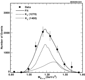
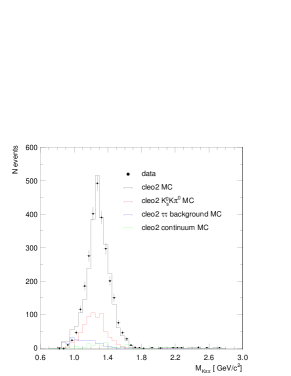
Figure 7: Mass distributions from tau decay modes containing kaons. Top: $M(K^{0}_{S}\pi^{-})$ from $\tau^{-}\to K^{0}_{S}\pi^{-}\nu_{\tau}$ [41]. Middle: $M(K\pi\pi)$ from $\tau^{-}\to K^{-}\pi^{+}\pi^{+}\nu_{\tau}$ [46]. Bottom: $M(K\pi\pi)$ from $\tau^{-}\to K^{0}_{S}\pi^{-}\pi^{0}\nu_{\tau}$ [41]. The data are shown as data points, and the topmost curve or histogram shows a model of the tau decay signal.

7.1 $\tau^{-}\to K_{1}^{-}\nu_{\tau}$ structure

The decay $\tau^{-}\to(K\pi\pi)^{-}\nu_{\tau}$ has particularly interesting structure. It can be studied in the final states $K^{-}\pi^{+}\pi^{-}\nu_{\tau}$ and $K^{0}_{S}\pi^{-}\pi^{0}\nu_{\tau}$. CLEO has published results focusing on the former [46], despite the poor $K^{\pm}/\pi^{\pm}$ separation. Results on the latter mode, which is much cleaner and can be isolated event-by-event, are still in progress [41].

The $(K\pi\pi)^{-}$ final state is expected to be dominated by the axial-vector $K_{1}$ ($J^{P}=1^{+}$). There are two such states; in the quark model, they are $K_{a}$ in the ${}^{3}P_{1}$ octet, the strange partner of the $a_{1}(1260)$; and $K_{b}$ in the ${}^{1}P_{1}$ octet, the strange partner of the $b_{1}(1235)$. The $K_{b}$ couples to $W$ only through an SU(3)-violating “second-class” current. Both $K_{1}$’s decay to $K\pi\pi$ via $K^{*}\pi$ and $K\rho$, and they mix, via virtual states, into the physically observed $K_{1}(1270)$, $K_{1}(1400)$. So, we have weak coupling, SU(3)-violation, mixing, and decays to resonances. In addition, $(K\pi\pi)^{-}$ final state could proceed via a vector current, via the Wess-Zumino anomaly: $K^{*\prime}\to(K^{*}\pi,K\rho)\to K\pi\pi$ .

We can parameterize the $K_{1a}\leftrightarrow K_{1b}$ mixing via a mixing angle:

$$K_{1}(1400) = K_{a}\cos{\theta_{K}}-K_{b}\sin{\theta_{K}}$$

$$K_{1}(1270) = K_{a}\sin{\theta_{K}}+K_{b}\cos{\theta_{K}}$$

and the $SU(3)_{f}$ symmetry breaking via a parameter $\delta$:
$\tau\to W\to|K_{a}\rangle-\delta|K_{b}\rangle$
$|\delta|=(m_{s}-m_{u})/\sqrt{2}(m_{s}+m_{u})\approx 0.18$.
The branching fraction of the $\tau$ to the $K_{1}$’s can then be written in terms of these parameters:

$$\frac{{\cal B}(\tau\to K_{1}(1270)\nu)}{{\cal B}(\tau\to K_{1}(1400)\nu)}=\left|\frac{\sin{\theta_{K}}-\delta\cos{\theta_{K}}}{\cos{\theta_{K}}+\delta\sin{\theta_{K}}}\right|^{2}\times\Phi,$$

where $\Phi$ is some known (or estimatable) kinematical and phase space terms.

From the CLEO data [46], we obtain two possible solutions, depending upon the sign of $\delta$:

$$\theta_{K} =(69\pm 16\pm 19)^{\circ}~{}~{}~{}(\delta=0.18),$$

$$\theta_{K} =(49\pm 16\pm 19)^{\circ}~{}~{}~{}(\delta=-0.18).$$

These mixing angles are consistent with those obtained using only the $K_{1}$ widths and branching fractions [47].

7.2 $\tau^{-}\to(4\pi)^{-}\nu_{\tau}$

The $\tau\to 4\pi\nu_{\tau}$ decay is expected to proceed through the vector current $(J^{P}=1^{-})$, dominated by the $\rho$, $\rho^{\prime}$, $\rho^{\prime\prime}$… resonances. There are many sub-resonances that can contribute: $\omega\pi$, $\eta\pi$, $a_{1}\pi$. In the CLEO analysis [48], the spectral functions $v(m^{2}_{4\pi})$ and $v(m^{2}_{\omega\pi})$ were measured, and the $\omega\pi$ contribution was modeled with interfering $\rho$, $\rho^{\prime}$, $\rho^{\prime\prime}$… resonances (see Fig. 8). The resonant substructure was measured and modeled, showing clear evidence for $\omega\pi$ and $\rho\pi\pi$, and the latter is consistent with originating from $a_{1}\pi$, $a_{1}\to\rho\pi$.

The $4\pi$ spectral function must be known well in order to use this final state to kinematically constrain the $\nu_{\tau}$ mass from $\tau\to 4\pi\nu_{\tau}$ data; this is discussed in section 8.1. The $4\pi$ spectral function can also be compared with the isospin-rotated reactions $e^{+}e^{-}\to 2\pi^{+}2\pi^{-}$, $\pi^{+}\pi^{-}2\pi^{0}$ as a test of CVC [40].

The $4\pi$ final state can also proceed through the axial-vector current, which is expected to be dominated by the $b_{1}(1235)$: $\tau\to b_{1}\nu_{\tau}$, $b_{1}\to\omega\pi$. The $b_{1}$ has, however, the wrong G-parity to couple to the weak charged current; it is a second-class current. The resulting decay to $\omega\pi$ occurs via an S- or D-wave, instead of the $\rho\to\omega\pi$ P-wave. CLEO measured the angular distribution in this decay (Fig. 8) and found complete consistency with P-wave decay, setting a limit on the non-vector current contribution of less than 5.4% of the total at 90% CL.

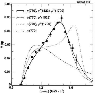
Figure 8: Distributions from $\tau^{-}\to\pi^{-}\pi^{+}\pi^{-}\pi^{0}\nu_{\tau}$ [48]. Top: The spectral function $v(M(\omega\pi))$, with fits to various combinations of $\rho$, $\rho^{\prime}$, $\rho^{\prime\prime}$… resonances. Bottom: Angular distribution sensitive to the polarization of the $\omega$ in $X\to\omega\pi$ (points), compared to predictions for different partial waves. Second-class currents would reveal themselves as $L=0,2$ partial waves.

8 Tau mass and lifetime, tau neutrino mass

CLEO pioneered the use of kinematical constraints to measure the tau mass, by observing semi-hadronic tau decays on both sides of an event, and determining for each event a maximum kinematically-allowed tau mass consistent with the observed hadronic energies and momenta. The distribution of this maximum mass exhibits a sharp drop-off near the tau mass, and from the position of this drop-off, CLEO measured [49] $m_{\tau}=(1778.2\pm 1.4)$ MeV.

At around the same time, the BES experiment measured the tau mass much more accurately, through a threshold scan [50]. CLEO turned this to an advantage; the “maximum kinematically-allowed tau mass” was really a measurement of a combination of the tau mass and the $\nu_{\tau}$ mass: $m_{\tau}^{kin}\simeq m_{\tau}^{BES}-m_{\nu_{\tau}}^{2}/m_{0}$ where $m_{0}$ is a mass parameter determined through Monte Carlo simulation. Making use of the BES measurement, CLEO kinematically constrained the $\nu_{\tau}$ mass to be $m(\nu_{\tau})<$ 60 MeV, 95% CL. Of course, what is being constrained here is the effective mass of the linear combination of neutrino mass eigenstates which couple to the tau.

CLEO-II used its vertex proportional chambers to measure the tau lifetime [51]. Using 1-v-3 and 3-v-3 events, and making use of vertex and beam position information, the tau lifetime was measured to be $\tau_{\tau}=289.0\pm 2.8\pm 4.0$ fs, in good agreement with more precise measurements from LEP. CLEO-II.V introduced a precision silicon vertex detector, but so far, that device has not been used to re-measure the tau lifetime.

8.1 Mass of the $m(\nu_{\tau})$

Regardless of $m(\nu_{\tau})$ constraints from $\nu$-mixing and cosmology, constraining it kinematically in tau decays remains a worthy goal. The ALEPH limit from 1998 still stands: $m^{eff}(\nu_{\tau})<18.2$ MeV (95% CL). (Again, what is being constrained here is the effective mass of the linear combination of neutrino mass eigenstates which couple to the tau.)

CLEO-II has published 3 limits on $m^{eff}(\nu_{\tau})$, using different decay modes and ever-larger datasets:
$m^{eff}(\nu_{\tau})<32.6$ MeV, 1993, $5\pi,3\pi 2\pi^{0}$ [52],
$m^{eff}(\nu_{\tau})<30$ MeV, 1998, $5\pi,3\pi 2\pi^{0}$ [53],
$m^{eff}(\nu_{\tau})<28$ MeV, 2000, $3\pi\pi^{0}$ [54].
The last two limits used the $M_{X}$ versus $E_{X}/E_{beam}$ technique pioneered at LEP, where $X$ is the hadronic system in $\tau\to X\nu_{\tau}$ decay. All three of these limits used a much larger data sample, than the one available to ALEPH, and comparable or better $M_{X}$, $E_{X}$ resolution. The data from the second analysis listed above is shown in Fig. 9.

If one is motivated to improve this kinematical limit appreciably, e.g. to approach the $\sim$ 1 MeV level, one needs lots of statistics, excellent, well-understood $M_{X}$, $E_{X}$ resolution, good spectral function models, and most especially, a good understanding of statistics and systematics - there are many subtleties [55]!

Figure 9: Distribution of invariant mass $M_{X}$ versus scaled energy $E_{X}/E_{beam}$ for $\tau\to X\nu_{\tau}$, where (a) $X=5\pi^{\pm}$, and (b) $X=3\pi^{\pm}2\pi^{0}$, in CLEO data [53] near the kinematic endpoints, with $1\sigma$ resolution error ellipses shown. The solid lines show the kinematical boundary for $m(\nu_{\tau})=0$, and the dashed contours are for $m(\nu_{\tau})=30$, 60, and 100 MeV.

9 CP Violation in tau decay

A highlight of the recent work in tau physics from CLEO has been the search for CP violation in tau decay [56].

Of course, CP violation is not expected in leptonic decays, in the Standard Model. To manifest it, a process must have two or more interfering amplitudes, with relatively complex phases (as in the CKM matrix in the quark sector). In the Standard Model, the $\mu$ and $\tau$ decay via one amplitude: $\tau^{-}\to W^{-}\nu_{\tau}$, a process that has been well studied at CLEO and LEP. Also, the charged leptons cannot undergo particle-antiparticle oscillations.

To produce CP violation in tau decay, we can add a second amplitude, such as a charged Higgs: $\tau^{-}\to H^{-}\nu_{\tau}$. Endow it with a complex coupling $\Lambda$ with a phase which flips sign under CP, and a strong phase (supplied by the $W\to\rho$ or $K^{*}$ Breit-Wigner propagator) which does not. CLEO has recently searched for CP violation due to such a mechanism, in two analyses.

In the first, the decay $\tau^{-}\to(K\pi)^{-}\nu_{\tau}$ (or its charged conjugate) is reconstructed on one side of the event. The other tau decay is used only to tag the event as $\tau^{+}\tau^{-}$. CP violation would manifest itself if the $K$ momentum vector lay preferentially on one side of the plane formed by the $e^{+}\tau^{+}$ momentum vectors; this effect is manifestly SU(3)_f violating.

In the second, both sides of the event are required to go to $\rho\nu_{\tau}$: $\tau^{+}\tau^{-}\to(\rho^{-}\nu_{\tau})(\rho^{+}\overline{\nu}_{\tau})$. The $\tau\to\rho\nu_{\tau}$ decays are used to analyze the spin orientation of each tau, and one looks for net transverse spin polarization; a manifestly isospin-violating, as well as CP-violating effect.

In both cases, maximal information about the presence of CP-violating terms in the decay rate (in the context of a model containing a scalar charged Higgs with a complex coupling $\Lambda$) is extracted by defining an optimal CP-violating observable, and looking for an asymmetry in the distribution of that observable.

No such asymmetry was seen, and (model-dependent) limits were set on $\Im(\Lambda)$:
$-0.172<\Im(\Lambda)<0.067$ at 90% CL
in the $\pi^{\pm}K^{0}_{S}\nu_{\tau}$ -vs- any-tag analysis [57], and
$-0.033<\Im(\Lambda)<0.089$ at 90% CL
in the $\rho^{+}\bar{\nu}$ -vs- $\rho^{-}\nu_{\tau}$ analysis [58].

9.1 Anomalous $\tau^{+}\tau^{-}$ production: dipole moments

As mentioned in section 2, it is of interest to search for anomalous $\tau^{+}\tau^{-}$ production at energies much below the $Z^{0}$, parameterized by anomalous dipole moments. The best sensitivity to anomalous dipole moments can be obtained by studying the spin correlations in $e^{+}e^{-}\to\gamma^{*}\to\tau^{+}\tau^{-}$ events.

Searches have recently been made by ARGUS [59] and Belle [60]. Sadly, CLEO has not published on this subject.

If the tau dipole moments are not anomalously large, then (far below the $Z^{0}$ peak) the taus in $\tau^{+}\tau^{-}$ events have very small net spin polarization. However, their spin polarizations are almost 100% correlated, in all three dimensions. This is interesting to measure, if only as as a test of QED.

The nature of spin correlations is a strong function of beam energy. At 10 GeV, tau pairs are produced via $e^{+}e^{-}\to\gamma^{*}$. This is parity-conserving, and at at energies where the taus are relativistic but not extremely so. Both longitudinal and transverse spin correlations are maintained, but there is no net spin polarization.

At LEP-I, tau pairs are produced via $e^{+}e^{-}\to Z^{0}$. This is parity-violating, and at energies where the taus are extremely relativistic. Both longitudinal and transverse spin correlations are maintained, but the large boost makes it nearly impossible to measure the transverse spin polarizations; and there is a net longitudinal spin polarization which is well established at LEP.

Near $\tau^{+}\tau^{-}$ threshold, tau pairs are produced via $e^{+}e^{-}\to\gamma^{*}$. Again, this is parity-conserving, but the taus are nearly at rest. The spin correlations are dominantly along the direction of the $e^{+}e^{-}$ beam axis. Again, there is no net spin polarization.

These differences lead to significant and interesting differences in the way anomalous dipole moments and CP violation are manifested in tau pair production, and different optimal observables must be defined in order to best observe it.

Figure 10: Illustration of tau spin correlations in $e^{+}e^{-}$ collisions at 10 GeV (top), near the peak of the $Z^{0}$ (middle), and near threshold (bottom).

10 Tau physics at CLEO-III and at CLEO-c

The study of tau physics continues in the CLEO-III era, where our RICH detector permits a more precise study of modes containing kaons [61].

CLEO-III has $9\times 10^{6}$ produced $\tau^{+}\tau^{-}$ near 10 GeV, with good $K/\pi$ separation. There is also $\sim 3\times 10^{6}$ fb^-1 collected on or near the peaks of the on $\Upsilon(nS)$ resonances ($n=1,2,3$) which will yield measurements of ${\cal B}(\Upsilon(nS)\to\tau^{+}\tau^{-})$. Other topics in tau physics which will be pursued include:

• rare decays, modes with kaons, precision measurements;

  More tests of CP in $\tau$ system: $h_{\nu_{\tau}}=-h_{\bar{\nu}_{\tau}}$;

  Rare decays may be seen: e.g., 2nd class currents;

  Limits (observation?) on LFV decays;

  anomalous (e.g., CPv) couplings in weak decay or in QED production;

  exotica (e.g., $\tau^{-}\to\pi^{-}\nu_{heavy}$, $e^{-}G^{0}$);

  continued testing and development of models of meson dynamics as a guide towards more fundamental theory: structure of $\tau\to 4\pi\nu_{\tau}$, $K3\pi\nu_{\tau}$, $\eta 2\pi\nu_{\tau}$, $\eta 3\pi\nu_{\tau}$, etc..

Within the next year, CESR will make the transition to CESR-c, operating in the $E_{cm}\sim 3-5$ GeV region. The suitably modified CLEO-c experiment will collect data on the $\psi(nS)$ resonances, and, hopefully, near/at $\tau^{+}\tau^{-}$ threshold. All the physics topics on the CLEO-III list above will also be accessible to CLEO-c, but with unique kinematical constraints [3].

When the taus are produced near threshold, decays like $\tau\to\pi\nu_{\tau}$ will produce a monochromatic pion, which will tag $\tau^{+}\tau^{-}$ events with good efficiency and virtually no background. It should be possible to measure branching fractions with sub-1% precision. It should be possible to obtain greater precision in measurements of the Michel parameters, especially the low-energy parameter $\eta$. The unique spin correlations near $\tau^{+}\tau^{-}$ threshold will permit new tests of QED, and facilitate searches for anomalous couplings. Threshold scans could result in measurements of the tau mass to a precision of 0.1 MeV. It may also be possible to limit $m(\nu_{\tau})$ kinematically at the $\sim$ 10 MeV level.

The CLEO-c tau-charm factory has a bright future in tau physics!

11 Summary

The CLEO Collaboration has published numerous studies of the physics of the tau lepton and its neutrino, and looks forward to continuing this work with data from the CLEO-III detector, and into the CLEO-c era.

The author would very much like to thank the organizers of Tau02 for their hospitality, but unfortunately, he was not able to avail himself of it, because personal problems prevented him from attending in person. He is grateful for the opportunity to give his presentation remotely.

References

- [1]
- [2] CLEO Collaboration (Y. Kubota, et al.), Nucl. Instr. Meth. 320, 66 (1992).
- [3] CESR-c Taskforce, CLEO-c Taskforce, and CLEO-c Collaboration, hep-ex/0205003, CLNS 01/1742 (2002).
- [4] CLEO Collaboration (D. Cinabro et al.), Phys. Lett. B 340, 129 (1994).
- [5] CLEO Collaboration (G. Crawford et al.), Nucl. Instr. Meth. A 345, 429 (1994).
-
[6]
S. Jadach et al., Comput. Phys. Commun. 130, 260 (2000);
S. Jadach et al., Phys. Rev. D 63, 113009 (2001);
See also http://jadach.home.cern.ch/jadach/
KKindex.html. - [7] Particle Data Group, R.M. Barnett et al., Phys. Rev. D 54, 1 (1994).
- [8] S. Jadach and Z. Was, Comput. Phys. Commun. 36, 191 (1985); and ibid, 64, 267 (1991); S. Jadach, J.H. Kühn, and Z. Was, Comput. Phys. Commun. 64, 275 (1991); ibid, 70, 69 (1992), ibid, 76, 361 (1993).
- [9] CLEO Collaboration (A. Anastassov et al.), Phys. Rev. D 55, 2559 (1997).
- [10] CLEO Collaboration (M. Artuso et al.), Phys. Rev. Lett. 72, 3762 (1994).
- [11] CLEO Collaboration (M. Procario et al.), Phys. Rev. Lett. 70, 1207 (1993).
- [12] CLEO Collaboration (R. Balest et al.), Phys. Rev. Lett. 75, 3809 (1995).
- [13] Particle Data Group, R. M. Barnett et al., Phys. Rev. D 54, 1 (1996).
- [14] CLEO Collaboration (D. Bortoletto et al.), Phys. Rev. Lett. 71, 1791 (1993).
- [15] CLEO Collaboration (D. Gibaut et al.), Phys. Rev. Lett. 73, 934 (1994).
- [16] CLEO Collaboration (S. Anderson et al.), Phys. Rev. Lett. 79, 3814 (1997).
- [17] CLEO Collaboration (A. Anastassov et al.), Phys. Rev. Lett. 86, 4467 (2001).
- [18] CLEO Collaboration (K.W. Edwards et al.), Phys. Rev. D 56, R5297 (1997).
- [19] CLEO Collaboration (M. Artuso et al.), Phys. Rev. Lett. 69, 3278 (1992).
- [20] CLEO Collaboration (J. Bartelt et al.), Phys. Rev. Lett. 76, 4119 (1996).
- [21] CLEO Collaboration (T. Bergfeld et al.), Phys. Rev. Lett. 79, 2406 (1997).
- [22] CLEO Collaboration (M. Bishai et al.), Phys. Rev. Lett. 82, 281 (1999).
- [23] CLEO Collaboration (T. Bergfeld et al.), Phys. Rev. Lett. 84, 830 (2000).
- [24] CLEO Collaboration (M.S. Alam et al.), Phys. Rev. Lett. 76, 2637 (1996).
- [25] CLEO Collaboration (A. Bean et al.), Phys. Rev. Lett. 70, 138 (1993).
- [26] CLEO Collaboration (K.W. Edwards et al.), Phys. Rev. D 55, R3919 (1997).
- [27] CLEO Collaboration (S. Ahmed et al.), Phys. Rev. D 61, 071101 (R)(2000).
- [28] CLEO Collaboration (J. Bartelt et al.), Phys. Rev. Lett. 73, 1890 (1994).
- [29] CLEO Collaboration (D.W. Bliss et al.), Phys. Rev. D 57, 5903 (1998).
- [30] CLEO Collaboration (G. Bonvicini et al.), Phys. Rev. Lett. 79, 1221 (1997).
- [31] CLEO Collaboration (R. Godang et al.), Phys. Rev. D 59, 091303 (1999).
- [32] CLEO Collaboration (S. Chen et al.), CLNS 02/1975, CLEO 02-12 (submitted to Phys.Rev.D).
- [33] CLEO Collaboration (R. Ammar et al.), Phys. Rev. Lett. 78, 4686 (1997).
- [34] CLEO Collaboration (T.E. Coan et al.), Phys. Rev. D 55, 7291 (1997).
- [35] CLEO Collaboration (J.P. Alexander et al.), Phys. Rev. D 56, 5320 (1997).
- [36] CLEO Collaboration (D.M. Asner et al.), Phys. Rev. D 61, 012002 (2000).
- [37] M. Davier, S. Eidelman, A. Hocker, Z. Zhang, hep-ph/0208177 (2002). See also the contribution by M. Davier to this conference.
- [38] CLEO Collaboration (T. Coan et al.), Phys. Lett. B 356, 580 (1995).
- [39] CLEO Collaboration (S. Anderson et al.), Phys. Rev. D 61, 112002 (2000).
- [40] See the contribution by S. Eidelman to this conference.
- [41] J. Smith, representing the CLEO Collaboration, in Proceedings of the Third Workshop on Tau Lepton Physics (1994), Nucl. Phys. B 40, 351 (1995). Never published in a refereed journal; work in progress.
- [42] CLEO Collaboration (T.E. Browder et al.), Phys. Rev. D 61, 052004 (2000).
- [43] See the contribution by E. Shibata to this conference.
- [44] CLEO Collaboration (M. Battle et al.), Phys. Rev. Lett. 73, 1079 (1994). CLEO Collaboration (T.E. Coan et al.), Phys. Rev. D 53, 6037 (1996).
- [45] CLEO Collaboration (S. Richichi et al.), Phys. Rev. D 60, 112002 (1999).
- [46] CLEO Collaboration (D. Asner et al.), Phys. Rev. D 62, 072006 (2000).
- [47] M. Suzuki, Phys. Rev. D 47, 1252 (1993).
- [48] CLEO Collaboration (K.W. Edwards et al.), Phys. Rev. D 61, 072003 (2000).
- [49] CLEO Collaboration (R. Balest et al.), Phys. Rev. D 47, R3671 (1993).
- [50] BES Collaboration (J.Z. Bai et al.), Phys. Rev. D 53, 20 (1996).
- [51] CLEO Collaboration (R. Balest et al.), Phys. Lett. B 388, 402 (1996).
- [52] CLEO Collaboration (D. Cinabro et al.), Phys. Rev. Lett. 70, 3700 (1993).
- [53] CLEO Collaboration (R. Ammar et al.), Phys. Lett. B 431, 209 (1998).
- [54] CLEO Collaboration (M. Athanas et al.), Phys. Rev. D 61, 052002 (2000).
- [55] J. Duboscq, in Proceedings of the Sixth Workshop on Tau Lepton Physics (2000), Nucl. Phys. B 98, 48 (2001).
- [56] R. Stroynowski, representing the CLEO Collaboration, contribution to this conference.
- [57] CLEO Collaboration (G. Bonvicini et al.), Phys. Rev. Lett. 88, 111803 (2002). This result supercedes: CLEO Collaboration (S. Anderson et al.), Phys. Rev. Lett. 81, 3823 (1998).
- [58] CLEO Collaboration (P. Avery et al.), Phys. Rev. D 64, 092005 (2001).
- [59] ARGUS Collaboration (H. Albrecht et al.), Phys. Lett. B 485, 37 (2000).
- [60] Belle Collaboration, BELLE-CONF-0250 (2001), and K. Inami, representing the Belle Collaboration, contribution to this conference.
- [61] F. Liu, representing the CLEO Collaboration, contribution to this conference.