EUROPEAN ORGANIZATION FOR NUCLEAR RESEARCH

CERN-EP/2002-059

23rd July 2002

Search for the Standard Model Higgs Boson with the OPAL Detector at LEP

The OPAL Collaboration

Abstract

This paper summarises the search for the Standard Model Higgs boson in ${\mathrm{e}}^{+}{\mathrm{e}}^{-}$ collisions at centre-of-mass energies up to 209 GeV performed by the OPAL Collaboration at LEP. The consistency of the data with the background hypothesis and various Higgs boson mass hypotheses is examined. No indication of a signal is found in the data and a lower bound of 112.7 ${\mathrm{GeV}}/c^{2}$ is obtained on the mass of the Standard Model Higgs boson at the 95% CL.

To be submitted to the European Physical Journal C

The OPAL Collaboration

G. Abbiendi², C. Ainsley⁵, P.F. Åkesson³, G. Alexander²², J. Allison¹⁶, P. Amaral⁹, G. Anagnostou¹, K.J. Anderson⁹, S. Arcelli², S. Asai²³, D. Axen²⁷, G. Azuelos^18,a, I. Bailey²⁶, E. Barberio⁸, R.J. Barlow¹⁶, R.J. Batley⁵, P. Bechtle²⁵, T. Behnke²⁵, K.W. Bell²⁰, P.J. Bell¹, G. Bella²², A. Bellerive⁶, G. Benelli⁴, S. Bethke³², O. Biebel³¹, I.J. Bloodworth¹, O. Boeriu¹⁰, P. Bock¹¹, D. Bonacorsi², M. Boutemeur³¹, S. Braibant⁸, L. Brigliadori², R.M. Brown²⁰, K. Buesser²⁵, H.J. Burckhart⁸, S. Campana⁴, R.K. Carnegie⁶, B. Caron²⁸, A.A. Carter¹³, J.R. Carter⁵, C.Y. Chang¹⁷, D.G. Charlton^1,b, A. Csilling^8,g, M. Cuffiani², S. Dado²¹, G.M. Dallavalle², S. Dallison¹⁶, A. De Roeck⁸, E.A. De Wolf⁸, K. Desch²⁵, B. Dienes³⁰, M. Donkers⁶, J. Dubbert³¹, E. Duchovni²⁴, G. Duckeck³¹, I.P. Duerdoth¹⁶, E. Elfgren¹⁸, E. Etzion²², F. Fabbri², L. Feld¹⁰, P. Ferrari⁸, F. Fiedler³¹, I. Fleck¹⁰, M. Ford⁵, A. Frey⁸, A. Fürtjes⁸, P. Gagnon¹², J.W. Gary⁴, G. Gaycken²⁵, C. Geich-Gimbel³, G. Giacomelli², P. Giacomelli², M. Giunta⁴, J. Goldberg²¹, E. Gross²⁴, J. Grunhaus²², M. Gruwé⁸, P.O. Günther³, A. Gupta⁹, C. Hajdu²⁹, M. Hamann²⁵, G.G. Hanson⁴, K. Harder²⁵, A. Harel²¹, M. Harin-Dirac⁴, M. Hauschild⁸, J. Hauschildt²⁵, C.M. Hawkes¹, R. Hawkings⁸, R.J. Hemingway⁶, C. Hensel²⁵, G. Herten¹⁰, R.D. Heuer²⁵, J.C. Hill⁵, K. Hoffman⁹, R.J. Homer¹, D. Horváth^29,c, R. Howard²⁷, P. Hüntemeyer²⁵, P. Igo-Kemenes¹¹, K. Ishii²³, H. Jeremie¹⁸, P. Jovanovic¹, T.R. Junk⁶, N. Kanaya²⁶, J. Kanzaki²³, G. Karapetian¹⁸, D. Karlen⁶, V. Kartvelishvili¹⁶, K. Kawagoe²³, T. Kawamoto²³, R.K. Keeler²⁶, R.G. Kellogg¹⁷, B.W. Kennedy²⁰, D.H. Kim¹⁹, K. Klein¹¹, A. Klier²⁴, S. Kluth³², T. Kobayashi²³, M. Kobel³, S. Komamiya²³, L. Kormos²⁶, R.V. Kowalewski²⁶, T. Krämer²⁵, T. Kress⁴, P. Krieger^6,l, J. von Krogh¹¹, D. Krop¹², K. Kruger⁸, M. Kupper²⁴, G.D. Lafferty¹⁶, H. Landsman²¹, D. Lanske¹⁴, J.G. Layter⁴, A. Leins³¹, D. Lellouch²⁴, J. Letts¹², L. Levinson²⁴, J. Lillich¹⁰, S.L. Lloyd¹³, F.K. Loebinger¹⁶, J. Lu²⁷, J. Ludwig¹⁰, A. Macpherson^28,i, W. Mader³, S. Marcellini², T.E. Marchant¹⁶, A.J. Martin¹³, J.P. Martin¹⁸, G. Masetti², T. Mashimo²³, P. Mättig^m, W.J. McDonald²⁸, J. McKenna²⁷, T.J. McMahon¹, R.A. McPherson²⁶, F. Meijers⁸, P. Mendez-Lorenzo³¹, W. Menges²⁵, F.S. Merritt⁹, H. Mes^6,a, A. Michelini², S. Mihara²³, G. Mikenberg²⁴, D.J. Miller¹⁵, S. Moed²¹, W. Mohr¹⁰, T. Mori²³, A. Mutter¹⁰, K. Nagai¹³, I. Nakamura²³, H.A. Neal³³, R. Nisius⁸, S.W. O’Neale¹, A. Oh⁸, A. Okpara¹¹, M.J. Oreglia⁹, S. Orito²³, C. Pahl³², G. Pásztor^4,g, J.R. Pater¹⁶, G.N. Patrick²⁰, J.E. Pilcher⁹, J. Pinfold²⁸, D.E. Plane⁸, B. Poli², J. Polok⁸, O. Pooth¹⁴, M. Przybycień^8,n, A. Quadt³, K. Rabbertz⁸, C. Rembser⁸, P. Renkel²⁴, H. Rick⁴, J.M. Roney²⁶, S. Rosati³, Y. Rozen²¹, K. Runge¹⁰, K. Sachs⁶, T. Saeki²³, O. Sahr³¹, E.K.G. Sarkisyan^8,j, A.D. Schaile³¹, O. Schaile³¹, P. Scharff-Hansen⁸, J. Schieck³², T. Schörner-Sadenius⁸, M. Schröder⁸, M. Schumacher³, C. Schwick⁸, W.G. Scott²⁰, R. Seuster^14,f, T.G. Shears^8,h, B.C. Shen⁴, C.H. Shepherd-Themistocleous⁵, P. Sherwood¹⁵, G. Siroli², A. Skuja¹⁷, A.M. Smith⁸, R. Sobie²⁶, S. Söldner-Rembold^10,d, S. Spagnolo²⁰, F. Spano⁹, A. Stahl³, K. Stephens¹⁶, D. Strom¹⁹, R. Ströhmer³¹, S. Tarem²¹, M. Tasevsky⁸, R.J. Taylor¹⁵, R. Teuscher⁹, M.A. Thomson⁵, E. Torrence¹⁹, D. Toya²³, P. Tran⁴, T. Trefzger³¹, A. Tricoli², I. Trigger⁸, Z. Trócsányi^30,e, E. Tsur²², M.F. Turner-Watson¹, I. Ueda²³, B. Ujvári^30,e, B. Vachon²⁶, C.F. Vollmer³¹, P. Vannerem¹⁰, M. Verzocchi¹⁷, H. Voss⁸, J. Vossebeld^8,h, D. Waller⁶, C.P. Ward⁵, D.R. Ward⁵, P.M. Watkins¹, A.T. Watson¹, N.K. Watson¹, P.S. Wells⁸, T. Wengler⁸, N. Wermes³, D. Wetterling¹¹ G.W. Wilson^16,k, J.A. Wilson¹, G. Wolf²⁴, T.R. Wyatt¹⁶, S. Yamashita²³, D. Zer-Zion⁴, L. Zivkovic²⁴

¹School of Physics and Astronomy, University of Birmingham, Birmingham B15 2TT, UK
²Dipartimento di Fisica dell’ Università di Bologna and INFN, I-40126 Bologna, Italy
³Physikalisches Institut, Universität Bonn, D-53115 Bonn, Germany
⁴Department of Physics, University of California, Riverside CA 92521, USA
⁵Cavendish Laboratory, Cambridge CB3 0HE, UK
⁶Ottawa-Carleton Institute for Physics, Department of Physics, Carleton University, Ottawa, Ontario K1S 5B6, Canada
⁸CERN, European Organisation for Nuclear Research, CH-1211 Geneva 23, Switzerland
⁹Enrico Fermi Institute and Department of Physics, University of Chicago, Chicago IL 60637, USA
¹⁰Fakultät für Physik, Albert-Ludwigs-Universität Freiburg, D-79104 Freiburg, Germany
¹¹Physikalisches Institut, Universität Heidelberg, D-69120 Heidelberg, Germany
¹²Indiana University, Department of Physics, Swain Hall West 117, Bloomington IN 47405, USA
¹³Queen Mary and Westfield College, University of London, London E1 4NS, UK
¹⁴Technische Hochschule Aachen, III Physikalisches Institut, Sommerfeldstrasse 26-28, D-52056 Aachen, Germany
¹⁵University College London, London WC1E 6BT, UK
¹⁶Department of Physics, Schuster Laboratory, The University, Manchester M13 9PL, UK
¹⁷Department of Physics, University of Maryland, College Park, MD 20742, USA
¹⁸Laboratoire de Physique Nucléaire, Université de Montréal, Montréal, Quebec H3C 3J7, Canada
¹⁹University of Oregon, Department of Physics, Eugene OR 97403, USA
²⁰CLRC Rutherford Appleton Laboratory, Chilton, Didcot, Oxfordshire OX11 0QX, UK
²¹Department of Physics, Technion-Israel Institute of Technology, Haifa 32000, Israel
²²Department of Physics and Astronomy, Tel Aviv University, Tel Aviv 69978, Israel
²³International Centre for Elementary Particle Physics and Department of Physics, University of Tokyo, Tokyo 113-0033, and Kobe University, Kobe 657-8501, Japan
²⁴Particle Physics Department, Weizmann Institute of Science, Rehovot 76100, Israel
²⁵Universität Hamburg/DESY, Institut für Experimentalphysik, Notkestrasse 85, D-22607 Hamburg, Germany
²⁶University of Victoria, Department of Physics, P O Box 3055, Victoria BC V8W 3P6, Canada
²⁷University of British Columbia, Department of Physics, Vancouver BC V6T 1Z1, Canada
²⁸University of Alberta, Department of Physics, Edmonton AB T6G 2J1, Canada
²⁹Research Institute for Particle and Nuclear Physics, H-1525 Budapest, P O Box 49, Hungary
³⁰Institute of Nuclear Research, H-4001 Debrecen, P O Box 51, Hungary
³¹Ludwig-Maximilians-Universität München, Sektion Physik, Am Coulombwall 1, D-85748 Garching, Germany
³²Max-Planck-Institute für Physik, Föhringer Ring 6, D-80805 München, Germany
³³Yale University, Department of Physics, New Haven, CT 06520, USA

^a and at TRIUMF, Vancouver, Canada V6T 2A3
^b and Royal Society University Research Fellow
^c and Institute of Nuclear Research, Debrecen, Hungary
^d and Heisenberg Fellow
^e and Department of Experimental Physics, Lajos Kossuth University, Debrecen, Hungary
^f and MPI München
^g and Research Institute for Particle and Nuclear Physics, Budapest, Hungary
^h now at University of Liverpool, Dept of Physics, Liverpool L69 3BX, UK
ⁱ and CERN, EP Div, 1211 Geneva 23
^j and Universitaire Instelling Antwerpen, Physics Department, B-2610 Antwerpen, Belgium
^k now at University of Kansas, Dept of Physics and Astronomy, Lawrence, KS 66045, USA
^l now at University of Toronto, Dept of Physics, Toronto, Canada
^m current address Bergische Universität, Wuppertal, Germany
ⁿ and University of Mining and Metallurgy, Cracow, Poland

1 Introduction

The $SU(2)_{L}\times U(1)_{Y}$ gauge theory of the electroweak interaction [1] accurately predicts all electroweak phenomena observed so far. It describes, with a minimum of assumptions, the structure of the electroweak gauge boson sector and its interactions with the fermions, and constrains the structure of the fermion multiplets. The gauge theory, $SU(2)_{L}\times U(1)_{Y}$, is referred to as the Standard Model (SM) of electroweak interactions. An important ingredient of the SM is the Higgs sector which provides masses for the gauge bosons $\mathrm{Z}$ and $\mathrm{W}^{\pm}$ and for the charged fermions without violating the principle of gauge invariance. This is done by introducing a doublet of scalar “Higgs” fields and their interaction [2]. One consequence of this extension is the prediction of a neutral scalar Higgs boson; its mass is a free parameter of the theory.

The SM predicts that Higgs bosons may be produced at ${\mathrm{e}}^{+}{\mathrm{e}}^{-}$ colliders via the Higgs-strahlung process, ${\mathrm{e}}^{+}{\mathrm{e}}^{-}$$\rightarrow$$\mathrm{H}$$\mathrm{Z}$. The cross-section depends only on the centre-of-mass energy $\sqrt{s}$ and the Higgs boson mass $m_{\mathrm{H}}$. Higgs bosons may also be produced via the $\mathrm{W}^{+}\mathrm{W}^{-}$ and $\mathrm{Z}\mathrm{Z}$ fusion processes ${\mathrm{e}}^{+}{\mathrm{e}}^{-}$$\rightarrow$$\mathrm{H}$$\nu_{\mathrm{e}}\bar{\nu_{\mathrm{e}}}$ and ${\mathrm{e}}^{+}{\mathrm{e}}^{-}$$\rightarrow$$\mathrm{H}$${\mathrm{e}}^{+}{\mathrm{e}}^{-}$. The same final states are also accessible via the Higgs-strahlung process and the contributions interfere. The diagrams for the Higgs-strahlung and fusion processes are shown in Figure 1. The fusion processes extend beyond the kinematic range of the Higgs-strahlung process. The fusion contributions are comparatively small at LEP2 energies, but taken into account in this analysis.

Previous searches performed by the OPAL Collaboration, at centre-of-mass energies up to 189 GeV, have excluded a Higgs boson with mass less than 91.0 ${\mathrm{GeV}}/c^{2}$ [3]. Using the data taken in the years 1999 and 2000 at $\sqrt{s}$ between 192 and 209 GeV, and based on a preliminary calibration of the detector and the beam energy, OPAL has raised this limit to 109.7 ${\mathrm{GeV}}/c^{2}$ [4].

This paper reports on the final results of the search for the Higgs boson, after the complete calibration, and supersedes the previous published results in [4]. Moreover, the analysis procedures have been modified to increase the search sensitivity in the mass region from 100 ${\mathrm{GeV}}/c^{2}$ up to about 115 ${\mathrm{GeV}}/c^{2}$. In this range, the Higgs boson is expected to decay predominantly to $\mathrm{b}\bar{\mathrm{b}}$ (73% to 80%, depending on $m_{\mathrm{H}}$), and $\tau^{+}\tau^{-}$(7%), with the remaining branching fraction shared between $\mathrm{c}\bar{\mathrm{c}}$, gg , and off shell $\mathrm{W}^{+}\mathrm{W}^{-}$ decays. The final states arising from the Higgs-strahlung process are determined by these decay properties of the Higgs boson and by those of the associated $\mathrm{Z}$ boson. The searches, therefore, encompass the “four-jet” channel ($\mathrm{H}$$\mathrm{Z}$$\rightarrow$$\mathrm{b}\bar{\mathrm{b}}$$\mathrm{q}\bar{\mathrm{q}}$), the “missing-energy” channel ($\mathrm{H}$$\mathrm{Z}$$\rightarrow$$\mathrm{b}\bar{\mathrm{b}}$$\nu\bar{\nu}$), the “tau” channels ($\mathrm{H}$$\mathrm{Z}$$\rightarrow$$\mathrm{b}\bar{\mathrm{b}}$$\tau^{+}\tau^{-}$, $\tau^{+}\tau^{-}$$\mathrm{q}\bar{\mathrm{q}}$) and the “electron” and “muon” channels ($\mathrm{H}$$\mathrm{Z}$$\rightarrow$$\mathrm{b}\bar{\mathrm{b}}$${\mathrm{e}}^{+}{\mathrm{e}}^{-}$, $\mathrm{b}\bar{\mathrm{b}}$$\mu^{+}\mu^{-}$). The dominant backgrounds arise from quark-pair production $\mbox{${\mathrm{e}}^{+}{\mathrm{e}}^{-}$}\mbox{$\rightarrow$}\mbox{$\mathrm{q}\bar{\mathrm{q}}$}(\gamma)$ and four-fermion production including $\mathrm{W}^{+}\mathrm{W}^{-}$ and $\mathrm{Z}\mathrm{Z}$ production. In particular, the $\mathrm{Z}\mathrm{Z}$ background constitutes an irreducible background for $m_{\mathrm{H}}$ $\sim$ $m_{\mathrm{Z}}$ if one of the $\mathrm{Z}$ bosons decays to $\mathrm{b}\bar{\mathrm{b}}$.

Section 2 summarises the properties of the OPAL detector, the data samples, and Monte Carlo simulation. Event reconstruction and b-tagging tools, which are common to the searches in all channels, are described in Section 3. The event selections addressing separately the four final states are discussed in detail in Section 4. The statistical procedures to investigate the compatibility of the observation with the background hypothesis and various Higgs signal hypotheses are described in Section 5. Finally, the results are summarised in Section 6.

2 Detector, Data Samples, and Monte Carlo Simulations

The tracking and calorimetry systems of the OPAL detector have nearly complete solid angle coverage. The central tracking detector is placed in a uniform 0.435 Tesla axial magnetic field. The innermost part is occupied by a high-resolution silicon microstrip vertex (“microvertex”) detector [5] which surrounds the beam pipe and covers the polar angle range $|\cos\theta|<0.93$. This detector is followed by a high-precision vertex drift chamber, a large-volume jet chamber, and chambers to measure the $z$ coordinates along the particle trajectories. A lead-glass electromagnetic calorimeter with a presampler is located outside the magnet coil. In combination with the forward calorimeters, a forward ring of lead-scintillator modules (the “gamma catcher”), a forward scintillating tile counter [6, 7], and the silicon-tungsten luminometer [8], the calorimeters provide a geometrical acceptance down to 25 mrad from the beam direction. The silicon-tungsten luminometer measures the integrated luminosity using Bhabha scattering at small angles [9]. The iron return-yoke of the magnet is instrumented with streamer tubes and thin-gap chambers for hadron calorimetry. Finally, the detector is completed by several layers of muon chambers.

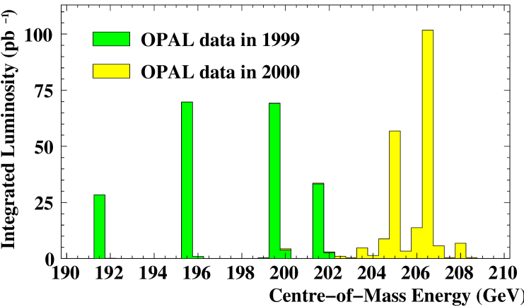
Figure 2: Integrated luminosity collected in the years 1999 and 2000, as a function of the centre-of-mass energy.

The data used for the present analysis were collected during the years 1999 and 2000 in ${\mathrm{e}}^{+}{\mathrm{e}}^{-}$ collisions at centre-of-mass energies between 192 and 209 GeV. During the year 2000 the LEP collider ran in a mode optimised for the highest possible luminosity at the highest available energies. The distribution of the integrated luminosity collected by OPAL at various LEP energies is shown in Figure 2 and summarised in Table 1.

A variety of Monte Carlo samples have been generated to estimate the detection efficiencies for the Higgs boson signal and to optimise the rejection of SM background processes. The cross-section and kinematic properties of the Higgs boson signal depend very strongly on $\sqrt{s}$ for Higgs boson masses near the limit of sensitivity. For an accurate modelling, the signal and background samples were generated at several centre-of-mass energies, from 192 GeV to 210 GeV, and in steps of 1 ${\mathrm{GeV}}/c^{2}$ from $m_{\mathrm{H}}$=80 ${\mathrm{GeV}}/c^{2}$ to $m_{\mathrm{H}}$=120 ${\mathrm{GeV}}/c^{2}$. For the Higgs boson signal the HZHA generator is used [10]. For the background processes the following event generators are used: KK2f [11] for $\mathrm{(Z/\gamma)}^{*}$$\rightarrow$$\mathrm{q}\bar{\mathrm{q}}$($\gamma$), $\mu^{+}\mu^{-}$$(\gamma)$ and $\tau^{+}\tau^{-}$$(\gamma)$, grc4f [12] for four-fermion processes (4f), BHWIDE [13] for ${\mathrm{e}}^{+}{\mathrm{e}}^{-}$$(\gamma)$, and PHOJET [14], HERWIG [15], and Vermaseren [16] for hadronic and leptonic two-photon processes ($\gamma\gamma$). JETSET [17] is used as the principal model for fragmentation. The detector response to the generated particles is simulated in full detail [18].

3 Event Reconstruction and B-Tagging

Some analysis procedures, described in this section, are common to all search channels. These include the reconstruction of particles and basic quality requirements, the assignment of particles to jets and the identification of jets which contain hadrons with b-flavour.

3.1 Particle Reconstruction Requirements

Events are reconstructed from charged-particle tracks and energy deposits (“clusters”) in the electromagnetic and hadronic calorimeters (the forward calorimeters are not used in the cluster reconstruction). Tracks have to satisfy the following quality requirements.

• The number of hits in the central jet chamber must exceed 20, and must be more than half the number of possible hits along the track, given its polar angle and origin.

• The polar angle of the track must satisfy $|\cos\theta|<0.962$.

• The distance of closest approach of the track to the beam axis must not exceed 2.5 cm.

• The $|z|$ coordinate of the track at the point of closest approach to the beam axis must not exceed 30 cm.

• The component of the momentum transverse to the beam axis must exceed 120 MeV$/c$.

Clusters have to satisfy the following quality requirements.

• At least one lead-glass block must contribute to an electromagnetic cluster in the barrel part of the electromagnetic calorimeter and at least two in the endcap part.

• These clusters must have an energy of at least 100 MeV in the barrel part and 250 MeV in the endcap part.

• Hadronic calorimeter clusters in the barrel or endcap parts must have an energy of at least 600 MeV; in the poletip hadron calorimeter the energy must exceed 2.0 GeV.

Charged particle tracks and energy clusters satisfying these quality requests are associated to form “energy flow objects”. A matching algorithm is employed to reduce double counting of energy in cases where charged tracks point towards electromagnetic clusters. Specifically, the expected calorimeter energy of the associated tracks is subtracted from the cluster energy. If the energy of a cluster is smaller than that expected for the associated tracks, the cluster is not used. Each accepted track and cluster is considered to be a particle. Tracks are assigned the pion mass. Clusters are assigned zero mass since they originate mostly from photons. The resulting energy flow objects are then grouped into jets and contribute to the total energy and momentum, $E_{\mathrm{vis}}$ and $P_{\mathrm{vis}}$, of the event. Unassociated tracks and clusters are left as single energy-flow objects. Corrections are applied to prevent multiple counting of energies in the case of particles which produce signals in several subdetectors. The association of energy flow objects (particles) into jets is provided primarily by the Durham jet finder algorithm [19] where the number of reconstructed jets in the event is controlled by the “jet resolution parameter” $y_{\mathrm{cut}}$. The value of $y_{\mathrm{cut}}$ is chosen in the various search channels according to the desired signal topology.

3.2 B-Tagging

We combine three nearly independent properties to identify jets containing b-hadron decays [3]: the high-$p_{t}$ lepton from the semi-leptonic decay $\mathrm{b\mbox{$\rightarrow$}c\ell^{\pm}\nu_{\ell}}$, the detectable lifetime of b-hadrons, and kinematic differences between b-decays and light-quark decays.

For each jet, using the jet-definition given by the channels, the outputs of the lifetime artificial neural network (ANN), the kinematic ANN, and the lepton tag are combined into a single likelihood variable ${\cal B}$.

• For the high-$p_{t}$ lepton tag, semileptonic b-decays are identified using electron and muon identification and rejection of $\mathrm{\gamma}$ conversions [20]. The high transverse momentum of the lepton with respect to the jet axis is used as a b-tag variable [21].

• The lifetime-sensitive tagging variables are combined to reconstruct secondary vertices. Tracks in the jet are ranked by an ANN (track-ANN) using the impact parameter of tracks with respect to the primary vertex. The first six tracks (or all tracks if their number is less than six) are used to form a “seed” vertex [22] by a technique where first a vertex is formed from all input tracks, and then the track with the highest contribution to the vertex $\chi^{2}$ is removed. This procedure is repeated until no track contributes more than 5 to the $\chi^{2}$, and the seed vertex is obtained by a fit to the selected tracks. After the seed vertex is formed, the remaining tracks in the jet are then tested, in the order of distance to the seed vertex, and added to this vertex if their contributions to the vertex $\chi^{2}$ are smaller than 5.

  In addition to identifying displaced vertices, we also use track impact parameters to gain further separation. The impact parameter significances $S^{r\phi}$ and $S^{rz}$, in the $r\phi$ and $rz$ projections, respectively, are formed by dividing the track impact parameters by their estimated errors. The distributions of $S^{r\phi}$ and $S^{rz}$ for each quark flavour, obtained from Z-peak Monte Carlo simulation, are used as the probability density functions (PDF’s) $f^{r\phi}_{q}$ and $f^{rz}_{q}$ ($q$=uds, c and b). The combined estimator $F_{q}$ for each quark flavour $q$ is computed by multiplying the $f^{r\phi}_{q}$ and $f^{rz}_{q}$ for all tracks. The final estimator ${\cal L}_{\mathrm{IP}}$ is obtained as the ratio of $F_{b}$ and the sum of $F_{uds}$, $F_{c}$ and $F_{b}$.

  The following four variables are used as inputs to the lifetime ANN.

  • The combined impact parameter likelihood ($\cal{L}_{\mathrm{IP}}$) described above.

  • The vertex significance likelihood ($\cal{L}_{\mathrm{V}}$): The likelihood for the vertex significance is computed analogously to the ${\cal L}_{\mathrm{IP}}$ above, using the decay length significance of the secondary vertex rather than the impact parameter significance of the tracks.

  • The reduced impact parameter likelihood ($\cal{R}_{\mathrm{IP}}$): To reduce sensitivity to single mismeasured tracks, the track with the largest impact parameter significance with respect to the primary vertex is removed from the secondary vertex candidate and the remaining tracks are used to recompute the likelihood $\cal{L}_{\mathrm{IP}}$. If the original vertex has only two tracks, the function is calculated from the impact parameter significance of the remaining track.

  • The reduced vertex significance likelihood ($\cal{R}_{\mathrm{V}}$). The track having the largest impact parameter significance is removed in the calculation of $\cal{L}_{\mathrm{V}}$.

• Three kinematic variables are combined in the jet-kinematics part of the tag, using an ANN: The number of energy-flow objects around the central part of the jet, the angle between the jet axis and its boosted sphericity axis, i.e. the sphericity [23] in the jet rest frame obtained by boosting back the system using the measured mass and momenta of the jet, and the $C$-parameter [27] for the jet boosted back to its rest frame.

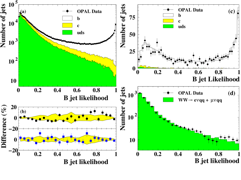
Figure 3: (a) The b-tagging algorithm output $\cal{B}$, for all jets in the $\mathrm{Z}$ calibration data. (b) The comparison between calibration data and simulation of the b-tag values opposite to an anti-tagged(upper part, dots) and a tagged(lower part, rectangles) b-jet. The shaded bands indicate the systematic uncertainty on the difference. (c) The distribution of $\cal{B}$ for high-energy ${\mathrm{e}}^{+}{\mathrm{e}}^{-}$$\rightarrow$$\mathrm{q}\bar{\mathrm{q}}$$(\gamma)$ events. One of the jets has been tagged as a b-jet and the $\cal{B}$ of the other jet is shown. (d) Distribution of $\cal{B}$ for jets in events identified as $\mbox{${\mathrm{e}}^{+}{\mathrm{e}}^{-}$}\mbox{$\rightarrow$}\mbox{$\mathrm{W}^{+}\mathrm{W}^{-}$}\mbox{$\rightarrow$}\mbox{$\mathrm{q}\bar{\mathrm{q}}$}\mathrm{e}\nu$ or $\mbox{$\mathrm{q}\bar{\mathrm{q}}$}\mu\nu$.

The outputs from the lifetime ANN, the high-$p_{t}$ lepton tag and the jet-kinematics ANN are combined with an unbinned likelihood calculation [21], and a final likelihood output ${\cal B}$ is computed for each jet. Figure 3 shows distributions of ${\cal B}$ obtained from various data sets. Figure 3(a) shows the distribution for data taken at $\sqrt{s}=m_{\mathrm{Z}}$ for calibration purposes [4], using the same detector configuration and operating conditions as for the high energy data. In this data set, the simulation reproduces the observed b-tagging efficiency within a precision of 1%, see Figure 3(b). The shaded band indicates the systematic uncertainties on the efficiency. In Figure 3(c), the distribution of ${\cal B}$ is shown for high energy data enriched in $\mathrm{(Z/\gamma)}^{*}$$\rightarrow{\mathrm{q\bar{q}}}$ processes with and without hard initial-state photon radiation. We find agreement with the SM Monte Carlo, within a relative statistical uncertainty of 5%. For the lighter flavours, the efficiency has been examined by vetoing b-flavoured jets in the opposite hemisphere, and the resulting estimate of the background is found to be described by Monte Carlo within a precision of 5–10%. In Figure 3(d) the distribution ${\cal B}$ for a high-purity sample of light-flavour jets in $\mathrm{W}^{+}\mathrm{W}^{-}$$\rightarrow$$\mathrm{q}\bar{\mathrm{q}}$$\ell\nu$ decays is shown.

4 Event Selection

For each of the four topological searches which may characterise $\mathrm{H}$$\mathrm{Z}$ signal events (see Section 1) the events are first required to pass a loose preselection. A finer selection is then applied using a likelihood function [24], or an ANN [25] with b-tagging and kinematic discriminating information as inputs. For the candidates passing the preselection, a reconstructed mass $m_{\mathrm{H}}^{\mathrm{rec}}$ is obtained. For each channel, two distributions are built for the expected signal, for the backgrounds and for the data. One is formed by mass dependent and the other by mass independent variables. For each Higgs mass to be tested, a discriminator, constructed as the product of these two distributions, is then fed into the statistical evaluation described in Section 5.2. Although the discriminator distributions are used in the confidence level calculations, a cut in the selection likelihood or ANN output is applied to evaluate the systematic uncertainties on the accepted rates and to illustrate the level of agreement between the data distributions and the Monte Carlo simulations (as shown in the figures and tables).

4.1 Four-Jet Channel

The four-jet channel selection is sensitive to the process ${\mathrm{e}}^{+}{\mathrm{e}}^{-}$$\rightarrow$$\mathrm{H}$$\mathrm{Z}$$\rightarrow$$\mathrm{b}\bar{\mathrm{b}}$$\mathrm{q}\bar{\mathrm{q}}$. The branching fraction of the $\mathrm{Z}$ to hadrons is approximately 70%, giving the four-jet channel a potentially large signal rate. The main backgrounds are hadronic $\mathrm{W}^{+}\mathrm{W}^{-}$ events, $\mathrm{Z}\mathrm{Z}$ events, and $\mbox{$\mathrm{q}\bar{\mathrm{q}}$}(\gamma)$ events in which two or more energetic gluons are radiated from the quarks. The b-tag removes nearly all of the $\mathrm{W}^{+}\mathrm{W}^{-}$ background, as well as much of the other backgrounds. The $\mathrm{Z}\mathrm{Z}$ background, with one $\mathrm{Z}$ decaying into $\mathrm{b}\bar{\mathrm{b}}$, is irreducible when searching for Higgs bosons of mass near $m_{\mathrm{Z}}$, but for higher masses the separation provided by the reconstructed mass, $m_{\mathrm{H}}^{\mathrm{rec}}$, becomes effective.

The Durham algorithm [19] is used to reconstruct four jets in each event; i.e., the resolution parameter $y_{\mathrm{cut}}$ is chosen to be between $y_{34}$ and $y_{45}$, where $y_{34}$ is the transition point from three to four jets, and $y_{45}$ is the transition point from four to five jets. These jets are used as reference jets in the following procedure. Each particle (energy flow object) is reassociated to the jet with the smallest “distance” to the particle. The “distance” is defined to be $E_{\mathrm{jet}}\cdot E_{\mathrm{particle}}\cdot(1-\cos{\theta})$, where $E_{\mathrm{jet}}$ is the energy of the reference jet, $E_{\mathrm{particle}}$ is the energy of the particle (energy-flow object) and $\theta$ is the angle between them. As a result of this procedure the di-jet mass resolution before kinematic fitting improves by about 10%.

4.1.1 Preselection

The preselection is designed to enrich the selected sample in four-jet events.

• Events must satisfy the standard hadronic final-state requirement [26].

• The effective centre-of-mass energy, $\sqrt{s^{\prime}}$, obtained by kinematic fits assuming that initial state radiation photons are lost in the beampipe or seen in the detector [26], must be at least 80% of $\sqrt{s}$.

• The value of $y_{34}$ must exceed 0.003.

• The event shape parameter $C$ [27] must be larger than 0.25.

• Each of the four jets must have at least two tracks.

• The $\chi^{2}$ probabilities must be larger than 10^-5 both for a four-constraint (4C) kinematic fit, which requires energy and momentum conservation, and for a five-constraint (5C) kinematic fit, $P_{\mathrm{HZ}}$, additionally constraining the invariant mass of one pair of jets to the mass of the $\mathrm{Z}$, $m_{{\mathrm{Z}}}$. The algorithm used to select the jet pair which is constrained to the $\mathrm{Z}$ mass is described below.

The numbers of events remaining after each preselection requirement are given in Table 2 for the data taken in 1999 and Table 3 for the data taken in 2000.

4.1.2 Jet-Pairing and Reconstructed Mass

There are six possible ways of grouping the four jets into pairs associated to two bosons. A likelihood method is used to choose the jet-pairing, where the combination with the highest likelihood value is retained for the final likelihood selection and the mass reconstruction. The correct assignment of particles to jets plays an essential role in accurately reconstructing the masses of the initial bosons.

The likelihood function is constructed from reference histograms for right and wrong pairing in signal and four-fermion background events. The signal samples used have 105 ${\mathrm{GeV}}/c^{2}$$<\mbox{$m_{\mathrm{H}}$}<$115 ${\mathrm{GeV}}/c^{2}$. All events in the $\mathrm{q}\bar{\mathrm{q}}$ background sample are classified as having wrong combinations.

The following six variables are used.

• The logarithm of the probability of a 5C kinematic fit constraining two of the jets to have an invariant mass $m_{\mathrm{Z}}$, $\log_{10}(P_{\mathrm{HZ}})$.

• ${\cal B}_{1}\cdot{\cal B}_{2}$, the product of the b-tagging discriminant variables for the two jets assumed to come from the Higgs boson decay.

• The quantity $(1-{\cal B}_{3})(1-{\cal B}_{4})$, formed from the b-tagging discriminant variables of the other two jets in the event.

• $|\cos\theta_{\mathrm{Z}}|$, where $\theta_{\mathrm{Z}}$ is the polar angle of the momentum sum of the two jets assigned to the Z.

• The 4C fit mass of the $\mathrm{Z}$ boson candidate, $m_{\mathrm{Z}}^{4C}$.

• The logarithm of the probability from a 6C fit, requiring energy and momentum conservation and constraining the masses of the pairs of jets to the WW hypothesis, $\log_{10}(P_{\mathrm{WW}})$.

For a signal of mass $m_{\mathrm{H}}$=115 ${\mathrm{GeV}}/c^{2}$, the fraction of swapped events is 7% (the two jets of the $\mathrm{H}$ incorrectly identified as originating from the $\mathrm{Z}$), and the fraction of correct-pairing is 58%, while for a sample of $\mathrm{Z}$$\mathrm{Z}$ ($\mathrm{W}^{+}\mathrm{W}^{-}$) events the correct-pairing fraction is 60% (75%).

Once the jet pairing is established, a Higgs boson mass is assigned to the event using $m_{\mathrm{H}}^{\mathrm{rec}}$$=m^{\mathrm{4C}}_{\mathrm{H}}+m^{\mathrm{4C}}_{\mathrm{Z}}-\mbox{$m_{\mathrm{Z}}$}$ where $m^{\mathrm{4C}}_{\mathrm{H}}$ and $m^{\mathrm{4C}}_{\mathrm{Z}}$ are the di-jet invariant masses of the assumed $\mathrm{H}$ and $\mathrm{Z}$ respectively. Hence the jet pairings which have the correct jet assignment to $\mathrm{Z}$/$\mathrm{H}$ and the swapped assignment have the same reconstructed mass.

4.1.3 Likelihood Selection

Events passing the preselection are assigned a discriminator function which is the product ${\cal D{\mathrm{(\mbox{$m_{\mathrm{H}}$})}}}={\cal L}_{1}\cdot{\cal L}_{2}$($m_{\mathrm{H}}$) of two separate likelihood functions. ${\cal L}_{1}$ is a likelihood using input variables which are not explicitly mass dependent, while ${\cal L}_{2}$($m_{\mathrm{H}}$) uses explicitly mass dependent characteristics of the event. To obtain ${\cal L}_{1}$ a set of signal samples with 105 ${\mathrm{GeV}}/c^{2}$$<$$m_{\mathrm{H}}$$<$115 ${\mathrm{GeV}}/c^{2}$ are combined into one sample, while the likelihood function ${\cal L}_{2}$($m_{\mathrm{H}}$) is obtained for individual $m_{\mathrm{H}}$ values in the range of 80 ${\mathrm{GeV}}/c^{2}$$<$$m_{\mathrm{H}}$$<$120 ${\mathrm{GeV}}/c^{2}$.

The input variables used in the likelihood ${\cal L}_{1}$ are listed below.

• ${\cal B}_{1}$ and ${\cal B}_{2}$, the b-tagging discriminant variable of the jet with the higher and lower energy assigned to the Higgs boson.

• The jet resolution parameter, $\log_{10}(y_{34})$.

• The event shape parameter $C$.

• $|\cos\theta_{\mathrm{Z}}|$ defined above in Section 4.1.2.

• $\log_{10}({P_{\mathrm{WW}}})$, for the dijet assignment chosen by the jet-pairing likelihood algorithm.

• $J_{s}$, the sum of the four smallest dijet angles.

• $\log_{10}(P_{\mathrm{HZ}})$, where $P_{\mathrm{HZ}}$ is the probability of a 5C kinematic fit constraining two of the jets to have invariant mass $m_{\mathrm{Z}}$. The two jets are those identified as the $\mathrm{Z}$ jets by the jet-pairing likelihood algorithm.

The input variables used in the likelihood ${\cal L}_{2}$ are:

• $M_{\mathrm{LH}}=(m^{\mathrm{rec}}_{\mathrm{H}}+91.2)/206$ ${\mathrm{GeV}}/c^{2}$, the scaled mass of the reconstructed hypothetical Higgs boson.

• $\beta_{\mathrm{min}}$, the minimum of $\beta_{\mathrm{dijet1}}+\beta_{\mathrm{dijet2}}$ for each of the possible dijet combinations, where $\beta_{\mathrm{dijet}}$ is the ratio of dijet momentum and energy after the 4C fit.

• $E_{\mathrm{diff}}=(E_{\mathrm{max}}-E_{\mathrm{min}})/\sqrt{s}$, the difference of the largest and the smallest jet energies normalised to the centre-of-mass energy.

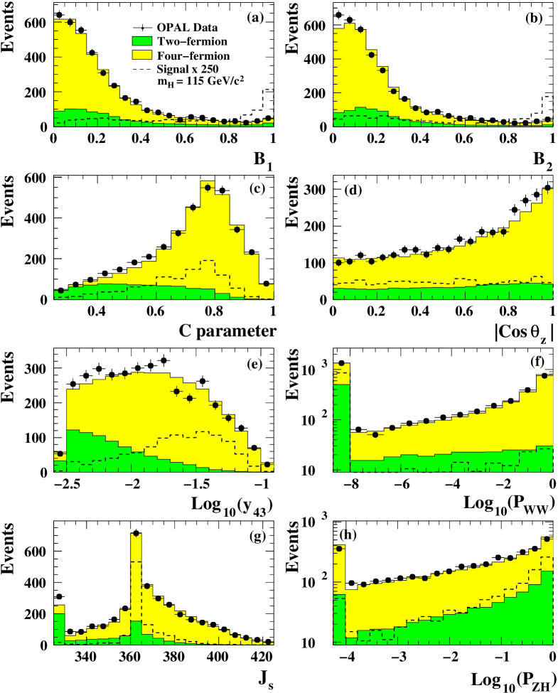
Figure 4: Four-Jet Channel: Distributions of the variables used as input to the likelihood function ${\cal{L}}_{1}$. Distributions of (a) ${\cal B}_{1}$ and (b) ${\cal B}_{2}$, (c) the $C$ parameter, (d) $|\cos\theta_{\mathrm{Z}}|$, (e) $\log_{10}(y_{34})$ using the Durham jet-finding algorithm, (f) $\log_{10}(P_{\mathrm{WW}})$, (g) jet-angle sum $J_{s}$, and (h) $\log_{10}(P_{\mathrm{HZ}})$.

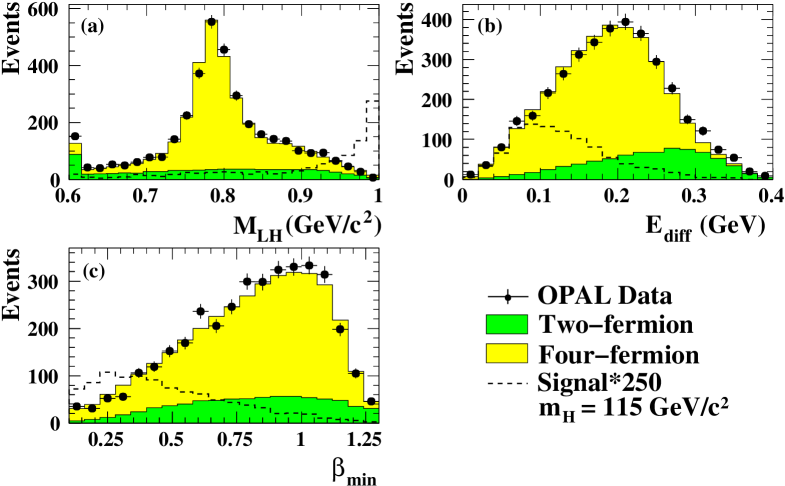
Figure 5: Four-Jet Channel: Distributions of the variables used as input to the likelihood function ${\cal L}_{2}$; (a) $\mathrm{M_{LH}}$, (b) $E_{\mathrm{diff}}$, and (c) $\beta_{\mathrm{min}}$.

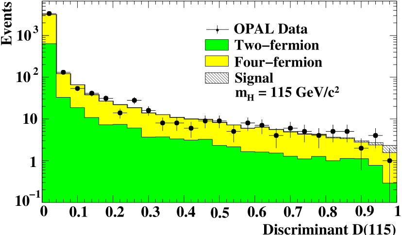
Figure 6: Four-Jet Channel: Distribution of the final discriminating function for a hypothetical $m_{\mathrm{H}}$=115 ${\mathrm{GeV}}/c^{2}$ signal added to the expectations from SM backgrounds.

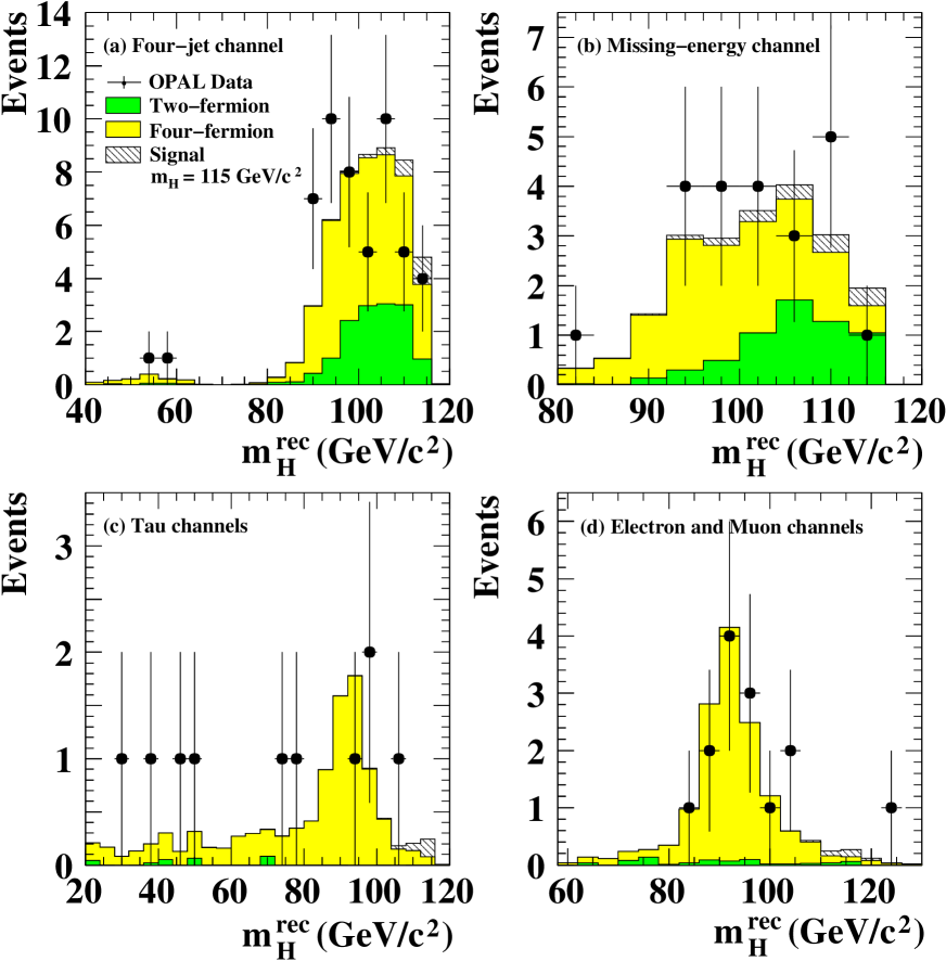
Figure 16: Distributions of the reconstructed mass for the selected events after a cut on the likelihood/ANN for (a) the four-jet channel, (b) the missing-energy channel, (c) the tau channels, and (d) the electron and muon channels combined.

The distributions of these input variables are shown in Figure 4 and Figure 5 for the data, the SM backgrounds and for a signal of mass $m_{\mathrm{H}}$=115 ${\mathrm{GeV}}/c^{2}$. The distributions of the resulting discriminator function are shown in Figure 6 and of the reconstructed Higgs boson mass in Figure 16(a) for the data, the SM background, and for a signal with $m_{\mathrm{H}}$=115 ${\mathrm{GeV}}/c^{2}$. For the purpose of this figure, ${\cal D{\mathrm{(\mbox{$m_{\mathrm{H}}$})}}}>0.54$ has been required. This cut retains 50 events in the data while 45.5$\pm$4.7 are expected on the basis of the SM background simulation.

4.2 Missing-Energy Channel

The ${\mathrm{e}}^{+}{\mathrm{e}}^{-}$$\rightarrow$$\mathrm{H}$$\mathrm{Z}$$\rightarrow$$\mathrm{b}\bar{\mathrm{b}}$$\nu\bar{\nu}$ process is characterised by a substantial amount of missing energy and a missing mass close to $m_{\mathrm{Z}}$. After preselection, an ANN is used to separate the signal from the background and forms the mass-independent part of the total discriminating variable. The mass dependent part is simply the reconstructed Higgs boson mass.

4.2.1 Preselection

The preselection is designed to remove accelerator-related backgrounds (such as beam-gas interactions and instrumental noise), dilepton final states, two-photon processes and radiative $\mathrm{q}\bar{\mathrm{q}}$ events, and to select events with a significant amount of missing energy. Events with large visible energy in the forward regions of the detector are also rejected since they are less well modelled and more likely to have mismeasured missing energies.

1. Dilepton final states and two-photon processes are reduced by the following requirements:

   • The number of tracks passing the quality requirements of Section 3 must be greater than six and must exceed 20% of the total number of reconstructed tracks.

   • No track momentum and no energy cluster in the electromagnetic calorimeter may exceed $\sqrt{s}/2$.

   • The visible energy must be less than 80% of $\sqrt{s}$.

   • The energy deposited in either side of the forward calorimeter must not exceed 2 GeV, and the energy deposits in either side of the silicon-tungsten luminometer and the gamma catcher must not exceed 5 GeV.

   • The component of the total visible momentum vector transverse to the beam axis must exceed 3 ${\mathrm{GeV}}/c$.

   • The visible mass must be greater than 4 ${\mathrm{GeV}}/c^{2}$, to suppress unmodelled two-photon events.

   • The thrust value $T$ must exceed 0.6.

   • The tracks and clusters in the event are grouped into two jets using the Durham algorithm. The $y_{\mathrm{cut}}$ at which the event changes its classification from a two-jet to a three-jet event, $y_{23}$, is required to be less than 0.3.

   • The chi-squared of the one-constraint (1C) HZ fit, $\chi^{2}_{\mathrm{HZ}}$, constraining the missing mass to $m_{\mathrm{Z}}$, is required to be less than 35.

2. The energy deposited in the forward region ($|\cos\theta|>0.9$) must not exceed 20% of the visible energy.

3. The missing mass must be in the range 50 ${\mathrm{GeV}}/c^{2}$$<M_{\mathrm{miss}}<130$ ${\mathrm{GeV}}/c^{2}$.

4. The effective centre-of-mass energy $\sqrt{s^{\prime}}$ [26] must exceed 60% of $\sqrt{s}$, to reject events with large amounts of initial-state radiation.

5. The acoplanarity angle ($180^{\circ}$ minus the angle between the two jets when projected into the $xy$ plane) must be between $3^{\circ}$ and $100^{\circ}$, to reject $\mathrm{q}\bar{\mathrm{q}}$ events, which often have nearly back-to-back jets.

6. The event must not have any identified isolated lepton [28], to reduce the background from $\mathrm{W}^{+}\mathrm{W}^{-}$ events.

7. To reduce background further, in particular $\mathrm{q}\bar{\mathrm{q}}$($\gamma$) background, the following cuts are applied:

   • The projection of the visible momentum along the beam axis, $|P^{z}_{\mathrm{vis}}|$, must not exceed 25% of $\sqrt{s}$.

   • The polar angle of the missing momentum vector must lie within the region $|\cos\theta_{\mathrm{miss}}|<0.95$ to reject radiative events and also to ensure that the missing momentum is not a result of mismeasurement.

   • The jet closest to the beam axis is required to have $|\cos\theta_{\mathrm{jet}}|<0.95$ to ensure complete reconstruction.

   • The polar angle of the thrust axis is required to satisfy $|\cos\theta_{\mathrm{thr}}|<0.95$ to ensure good containment of the event.

The numbers of events remaining after each selection requirement are given in Table 2 for the data taken in 1999 and in Table 3 for the data taken in 2000.

4.2.2 Neural Net Selection

The 13 variables used as inputs to the ANN are listed below. All variables are scaled to values between zero and one, and some of the variables with peaking distributions are subject to logarithmic transformations to give smoother distributions better suited for use as ANN input variables.

• The effective centre-of-mass energy $\sqrt{s^{\prime}}$  divided by $\sqrt{s}$,

• The missing mass $M_{\mathrm{miss}}$,

• The polar angle of the missing momentum vector $|\cos\theta_{\mathrm{miss}}|$,

• The thrust value, $\ln{(1-T)}$,

• The polar angle of the thrust axis $|\cos\theta_{\mathrm{thr}}|$,

• The jet resolution parameter, $\ln(y_{32})$,

• The acoplanarity angle of the jets, $\ln{(\phi_{\mathrm{acop}})}$,

• The polar angle of the jet closest to the beam pipe, $|\cos\theta_{\mathrm{jet}}|$,

• The b-tag likelihood output ${\cal B}_{1}$ of the more energetic jet,

• The b-tag likelihood output ${\cal B}_{2}$ of the less energetic jet,

• The angle between the more energetic jet and the missing momentum vector,
  $\ln(1-\cos\angle(j_{1},p_{\mathrm{miss}}))$,

• The angle between the less energetic jet and the missing momentum vector,
  $\cos\angle(j_{2},p_{\mathrm{miss}})$,

• The logarithm of the $\chi^{2}$ of the 1C HZ fit, $\ln(\chi^{2}_{\mathrm{HZ}}$).

The jet b-tag variables ${\cal B}_{1}$ and ${\cal B}_{2}$ differ from the ones described in Section 3.2 in that the high-$p_{t}$ lepton information is not used. Removing it from the b-tag reduces the rate at which $\mathrm{W}^{+}\mathrm{W}^{-}$$\rightarrow$$\mathrm{q\overline{q}^{\prime}}$$\ell\nu$ events with leptons close to or inside jets have spurious b-tags.

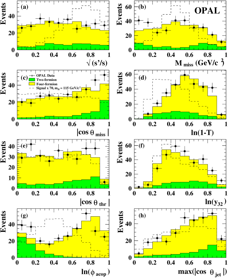
Figure 7: Missing-Energy Channel: Distributions of the variables used as inputs to the ANN. (a) $\sqrt{s^{\prime}/s}$, (b) $M_{\mathrm{miss}}$, (c) $|\cos\theta_{\mathrm{miss}}|$, (d) the logarithm of (1-$T$), (e) the cosine of the thrust polar angle, (f) the logarithm of $y_{32}$, (g) the logarithm of the acoplanarity, (h) the cosine of the polar angle of the jet closest to the beam pipe.

The distributions of the missing energy channel ANN input variables for the data, SM background and for a Higgs boson signal with $m_{\mathrm{H}}$=115 ${\mathrm{GeV}}/c^{2}$ are shown in Figures 7 and 8. The input values of each preselected event are passed on to an ANN, which is trained to give zero for background and one for signal events. The ANN’s were trained at three centre-of-mass energies, which cover the range of the data.

• At 196 GeV for year 1999 data with $\sqrt{s}=192$ and 196 GeV,

• At 200 GeV for year 1999 data with $\sqrt{s}=200$ and 202 GeV,

• At 207 GeV for all year 2000 data.

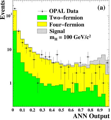
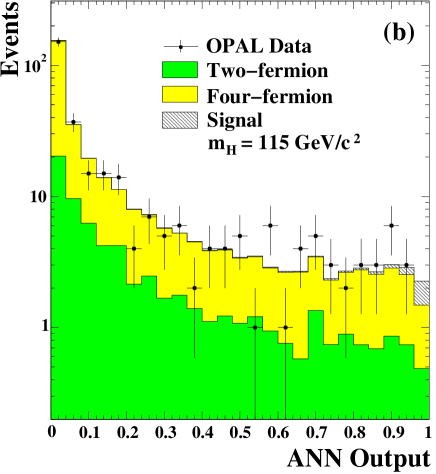
Figure 9: Missing-energy channel: Distribution of the outputs of the two different ANN’s. Plots (a) and (b) shows the output of the ANN trained with $m_{\mathrm{H}}$=100 ${\mathrm{GeV}}/c^{2}$ signal and $m_{\mathrm{H}}$=110 ${\mathrm{GeV}}/c^{2}$ signal, respectively.

At each energy, two separate ANNs were trained, one for low Higgs boson masses ($\mbox{$m_{\mathrm{H}}$}<107~{}\mbox{${\mathrm{GeV}}/c^{2}$}$), and one for high masses ($\mbox{$m_{\mathrm{H}}$}>107~{}\mbox{${\mathrm{GeV}}/c^{2}$}$). The Monte Carlo samples for training contained a full SM background simulation as well as Higgs signal with $m_{\mathrm{H}}$=100 ${\mathrm{GeV}}/c^{2}$ for the low-mass and $m_{\mathrm{H}}$=110 ${\mathrm{GeV}}/c^{2}$ for the high-mass ANN. Monte Carlo studies have shown this training strategy to be optimal. The output distributions of the two ANNs in data and Monte Carlo are shown in Figure 9(a) and  9(b) for the years 1999 and 2000.

A cut at ANN$>$0.7 has been used to calculate all systematic and statistical errors and is used in the tables and figures. This cut retains 21 events in the data while 22.8$\pm$2.7 are expected on the basis of the SM background simulation. Figure 16(b) shows the distributions of the reconstructed mass for the SM background and for an $m_{\mathrm{H}}$=115 ${\mathrm{GeV}}/c^{2}$ signal.

4.3 Tau Channels

The tau channel selection is sensitive to the two processes ${\mathrm{e}}^{+}{\mathrm{e}}^{-}$$\rightarrow$$\mathrm{H}$$\mathrm{Z}$$\rightarrow$$\mathrm{b}\bar{\mathrm{b}}$$\tau^{+}\tau^{-}$ and ${\mathrm{e}}^{+}{\mathrm{e}}^{-}$$\rightarrow$$\mathrm{H}$$\mathrm{Z}$$\rightarrow$$\tau^{+}\tau^{-}$$\mathrm{q}\bar{\mathrm{q}}$. The preselection is designed to identify events with two jets and two tau leptons. Efficient tau identification is important to separate the signal from the background which arises mainly from $\mbox{$\mathrm{q}\bar{\mathrm{q}}$}(\gamma)$, $\mathrm{Z}\mathrm{Z}$ and $\mathrm{W}^{+}\mathrm{W}^{-}$ processes, with either real tau leptons or with hadronic jets or isolated tracks with high transverse momentum misidentified as tau leptons. The two signal processes have different kinematic and b-tagging characteristics; therefore two likelihood functions are created, one optimised for each signal process. If the event passes the requirements for either of them, it is counted as a candidate event.

4.3.1 Tau Identification

The tau identification procedure [21] makes use of an ANN and combines the ANN outputs for two oppositely-charged tau candidates with a likelihood. The ANN is a track-based algorithm trained to discriminate real tau decay tracks from tracks arising from the hadronic system. Tracks were not considered if they had a ratio of the momentum resolution over the momentum, $\sigma_{p}/p$, larger than 0.5, if they passed within $1.5^{\circ}$ of a jet chamber anode plane or if they were identified as being consistent with coming from a photon conversion.

To construct the reference histograms a signal sample is used in which two bosons, both in the mass range of 20 to 170 ${\mathrm{GeV}}/c^{2}$, decay into $\tau^{+}\tau^{-}$$\mathrm{b}\bar{\mathrm{b}}$ so that the networks are trained on a wide variety of tau momenta. The background sample consists of ${\mathrm{e}}^{+}{\mathrm{e}}^{-}$$\rightarrow$$\mathrm{q}\bar{\mathrm{q}}$ events.

Any track with momentum greater than $2$ GeV$/c$ and with no other good track within a narrow cone of half-angle $10^{\circ}$ is considered as a one-prong tau candidate. Any family of exactly three charged tracks, having a total charge of $\pm 1$ and a total momentum greater than $2$ GeV$/c$, within a $10^{\circ}$ cone centred on the track with the highest momentum is considered as a three-prong tau candidate. Separate ANN’s were trained to identify one-prong and three-prong tau decays.

Around each candidate, an isolation cone of half-angle $30^{\circ}$ is constructed, concentric with and excluding the narrow $10^{\circ}$ cone. Both the one-prong and the three-prong ANN’s use as inputs the invariant mass of all tracks and neutral clusters (i.e. with no associated tracks) in the $10^{\circ}$ cone, the ratio of the total energy contained in the $30^{\circ}$ isolation cone to that in the $10^{\circ}$ cone, and the total number of tracks and neutral clusters with energy greater than $750$ MeV in the isolation cone. The one-prong ANN additionally takes as input the total energy in the $10^{\circ}$ cone, and the track energy in the isolation cone. The three-prong ANN additionally uses the largest angle between the most energetic track and any other track in the $10^{\circ}$ cone.

To select signal candidates, we use the two-tau likelihood [21],

$$\mathcal{L}_{\tau\tau}={{\frac{P_{1}P_{2}}{P_{1}P_{2}+(1-P_{1})(1-P_{2})}}},$$ (1)

where $P_{i}$ is the probability that the $i^{\mathrm{th}}$ tau candidate originates from a real tau lepton. This probability is calculated from the shapes of the ANN output for signal and fake taus. The distribution of the ANN output for signal events was computed from Monte Carlo simulations. The distribution of the ANN output in hadronic $\mathrm{Z}$ decay data collected in the calibration run at $\sqrt{s}\approx 91$ GeV, which has a low fraction of events with real taus, was used as the reference distribution for fake taus. This estimation of the fake tau rate from data reduces the corresponding systematic uncertainty. To pass the selection, an event must have $\mathcal{L}_{\tau\tau}$ of at least 0.10.

4.3.2 Preselection

The preselection requirements are as follows.

1. A basic selection is made to ensure well-measured events and reject accelerator backgrounds, dilepton events, two-photon events, and two-fermion events with ISR.

   • The event must satisfy the standard hadronic final state requirement [26].

   • To ensure that the selected events are well measured, the magnitude of the missing momentum $p_{\mathrm{miss}}$ has to be less than $0.3\mbox{$\sqrt{s}$}$.

   • The direction of the missing momentum must be well within the detector acceptance, $\left|\cos\theta_{\mathrm{miss}}\right|\leq 0.95$, in order to reject events with substantial ISR energy escaping undetected along the beam axis.

   • The scalar sum of the transverse momenta of the particles in the event must exceed 45 GeV$/c$.

2. At least one pair of oppositely charged tau candidates must be identified by the two-tau likelihood.

3. The particles in the events are subdivided into two tau candidates and two jets. A two-constraint kinematic fit is applied using total energy and momentum conservation constraints, where the tau momentum directions are taken from their visible decay products while leaving the energies free. The $\chi^{2}$-probability of the fit is required to be larger than $10^{-5}$.

4. In events where both taus are classified as one-prong decays, the sum of the momenta of the charged particles assigned to the tau decays must be less than 80 GeV$/c$, in order to reduce backgrounds from $\mbox{$\mathrm{Z}\mathrm{Z}$}\mbox{$\rightarrow$}\mu^{+}\mu^{-}\mbox{$\mathrm{q}\bar{\mathrm{q}}$}$ and $\mbox{$\mathrm{Z}\mathrm{Z}$}\mbox{$\rightarrow$}{\mathrm{e^{+}e^{-}}}\mbox{$\mathrm{q}\bar{\mathrm{q}}$}$.

4.3.3 Likelihood Selection

Two final likelihoods are then constructed from reference histograms. One of them, $\mathcal{L}(\mbox{$\mathrm{b}\bar{\mathrm{b}}$}\mbox{$\tau^{+}\tau^{-}$})$, is optimised for the $\mathrm{H}$$\mathrm{Z}$$\rightarrow$$\mathrm{b}\bar{\mathrm{b}}$$\tau^{+}\tau^{-}$ final state and makes use of the b-tag of Section 3.2. The other, $\mathcal{L}(\mbox{$\tau^{+}\tau^{-}$}\mbox{$\mathrm{q}\bar{\mathrm{q}}$})$, is optimised for the $\mathrm{H}$$\mathrm{Z}$$\rightarrow$$\tau^{+}\tau^{-}$$\mathrm{q}\bar{\mathrm{q}}$ process and does not use b-tagging. The following variables serve as inputs to both likelihoods:

• The ratio of the visible energy and the beam energy, $R_{\mathrm{vis}}$= $E_{\mathrm{vis}}$/$\sqrt{s}$,

• The polar angle of the missing momentum $\left|\cos\theta_{\mathrm{miss}}\right|$,

• $\log_{10}{(y_{34})}$, using the Durham algorithm, and allowing the tau candidates to be identified as low-multiplicity jets,

• The angles between each tau candidate and the nearest jet,

• The logarithm of the larger of two 3C kinematic fit probabilities, in which the additional constraint comes from fixing either the tau pair invariant mass or the jet pair invariant mass to the $\mathrm{Z}$ mass,

• The tau likelihood, $1-\sqrt{1-\mathcal{L}_{\tau\tau}}$,

• The energy of the most energetic electron or muon identified in the event (if any),

• $\sqrt{P_{\mathrm{joint}}}$, where $P_{\mathrm{joint}}$ is the probability that the $N$ tracks identified as the products of the tau decay come from the primary vertex. This is used to separate real taus from prompt electrons, muons and hadronic fake taus [29].

In addition to the above variables, the $\mathcal{L}(\mbox{$\mathrm{b}\bar{\mathrm{b}}$}\mbox{$\tau^{+}\tau^{-}$})$ likelihood uses as an input $1-\sqrt{1-{\cal B_{\tau}}}$, where

$${\cal B_{\tau}}=\frac{{\cal B}_{1}{\cal B}_{2}}{{\cal B}_{1}{\cal B}_{2}+(1-{\cal B}_{1})(1-{\cal B}_{2})},$$ (2)

and ${\cal B}_{1}$ and ${\cal B}_{2}$ are the b-tag discriminating variables described in Section 3.2 for the two hadronic jets in the event.

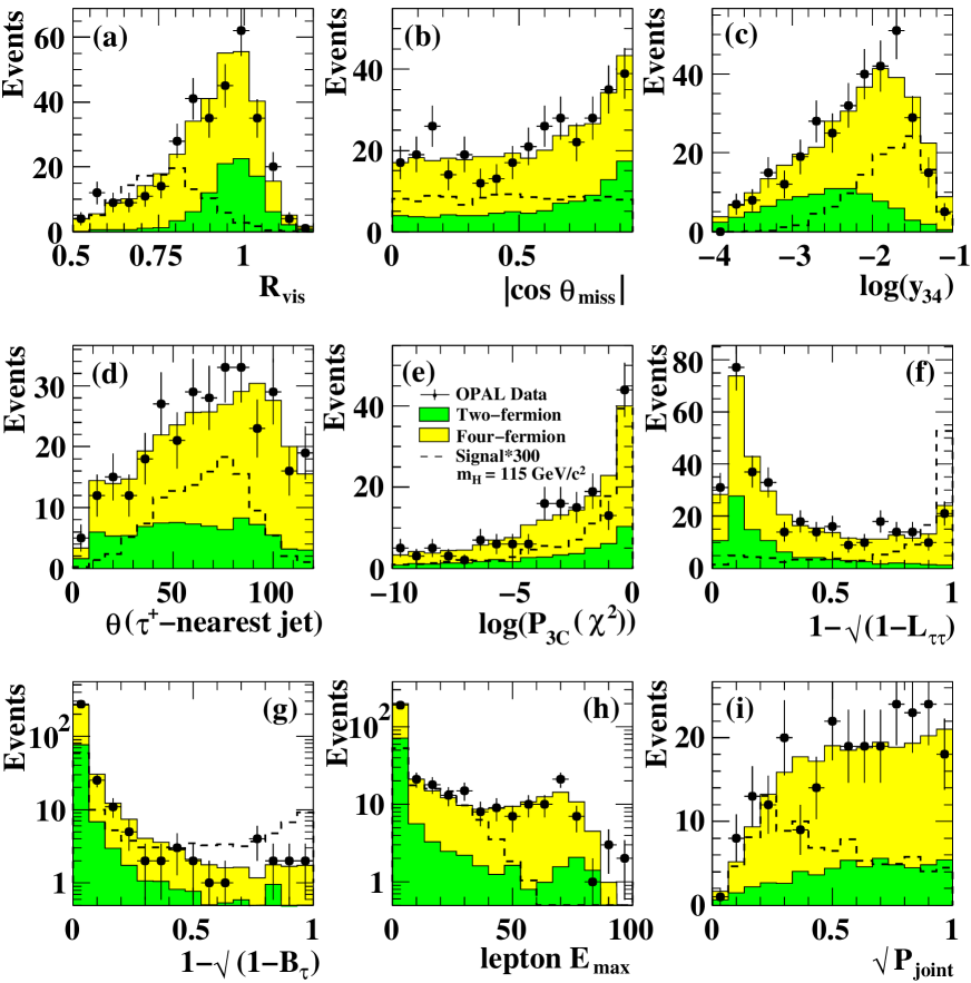
Figure 10: Tau channels: Distributions of the likelihood input variables, (a) $R_{\mathrm{vis}}$, (b) $|\cos\theta_{\mathrm{miss}}|$, (c) $\log_{10}(y_{34})$, (d) the angle between the $\tau^{+}$ candidate and the nearest jet in degrees, (e) the logarithm of the larger of two 3C fit probabilities, fixing either the dijet mass or the tau pair mass to $m_{\mathrm{Z}}$, (f) the combined tau likelihood, (g) the combined b-tag, (h) the lepton $E_{\mathrm{max}}$, and (i) $\sqrt{P_{\mathrm{joint}}}$.

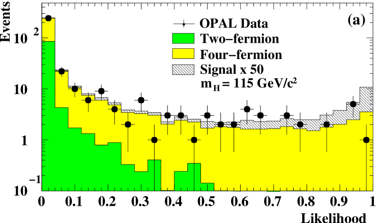
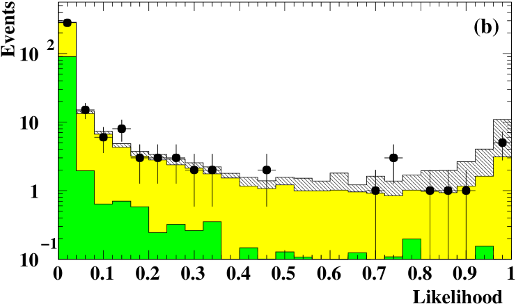
Figure 11: Tau channels: Distributions of the two likelihood output variables (a) ${\cal L}(\tau\tau\mbox{$\mathrm{q}\bar{\mathrm{q}}$})$ and (b) ${\cal L}(\mbox{$\mathrm{b}\bar{\mathrm{b}}$}\tau\tau)$.

The reference histograms for $\mathcal{L}(\mbox{$\mathrm{b}\bar{\mathrm{b}}$}\mbox{$\tau^{+}\tau^{-}$})$ include contributions only from signal and background events containing B hadrons, while the reference histograms for $\mathcal{L}(\mbox{$\tau^{+}\tau^{-}$}\mbox{$\mathrm{q}\bar{\mathrm{q}}$})$ include contributions only from events without B hadrons. Distributions of the likelihood input variables for the data, SM backgrounds, and a signal with $m_{\mathrm{H}}$=115 GeV, are shown in Figure 10 for the year 2000 data sample. The distributions of the likelihood discriminants $\mathcal{L}(\mbox{$\mathrm{b}\bar{\mathrm{b}}$}\mbox{$\tau^{+}\tau^{-}$})$ and $\mathcal{L}(\mbox{$\tau^{+}\tau^{-}$}\mbox{$\mathrm{q}\bar{\mathrm{q}}$})$ are shown in Figure 11. All events passing the preselection are retained for the calculation of the confidence levels.

As discussed in Section 4, the discriminator used for the confidence level calculation is composed of mass-dependent and mass-independent parts. In this channel, the reconstructed Higgs boson mass is used for the mass-dependent part, and either the $\mathrm{b}\bar{\mathrm{b}}$$\tau^{+}\tau^{-}$ or the $\tau^{+}\tau^{-}$$\mathrm{q}\bar{\mathrm{q}}$ likelihood is used for the mass-independent part. The choice of the likelihood is based on a study performed on $\mathrm{H}$$\mathrm{Z}$$\rightarrow$$\tau^{+}\tau^{-}$$\mathrm{q}\bar{\mathrm{q}}$ and $\mathrm{H}$$\mathrm{Z}$$\rightarrow$$\mathrm{b}\bar{\mathrm{b}}$$\tau^{+}\tau^{-}$ signal events. The distribution of the signal events in the $\mathcal{L}(\mbox{$\tau^{+}\tau^{-}$}\mbox{$\mathrm{q}\bar{\mathrm{q}}$})$ versus $\mathcal{L}(\mbox{$\mathrm{b}\bar{\mathrm{b}}$}\mbox{$\tau^{+}\tau^{-}$})$ plane shows two well separated regions. The likelihood to be used for each candidate is chosen according to the region of the likelihood plane in which it falls.

For the calculation of systematic errors and for illustration purposes in tables and figures, an event is selected as a candidate if either $\mathcal{L}(\mbox{$\mathrm{b}\bar{\mathrm{b}}$}\mbox{$\tau^{+}\tau^{-}$})>0.92$ or $\mathcal{L}(\mbox{$\tau^{+}\tau^{-}$}\mbox{$\mathrm{q}\bar{\mathrm{q}}$})>0.88$. The distributions of the reconstructed mass for the data, the Standard Model backgrounds, and a signal of mass $m_{\mathrm{H}}$=115 ${\mathrm{GeV}}/c^{2}$ are shown in Figure 16(c).

The numbers of observed and expected events after each stage of the selection are given in Table 2, together with the detection efficiency for a 100 ${\mathrm{GeV}}/c^{2}$ SM Higgs boson, for the data taken in 1999, and in Table 3, with the detection efficiency for a 115 ${\mathrm{GeV}}/c^{2}$ SM Higgs boson, for the data taken in 2000. Ten events survive the likelihood cut, to be compared to the expected background of $9.6\pm 1.1$.

4.4 Electron and Muon Channels

The signature for the Higgs signal in the light-lepton channels, ${\mathrm{e}}^{+}{\mathrm{e}}^{-}$$\rightarrow$$\mathrm{H}$$\mathrm{Z}$$\rightarrow$$\mathrm{b}\bar{\mathrm{b}}$${\mathrm{e}}^{+}{\mathrm{e}}^{-}$ and $\mathrm{b}\bar{\mathrm{b}}$$\mu^{+}\mu^{-}$, is two hadronic jets from the decay of the $\mathrm{H}$ and two leptons, either electrons or muons, from the decay of the $\mathrm{Z}$. The hadronic jets are expected to contain B hadrons, and the invariant mass of the leptons is expected to be close to the $\mathrm{Z}$ mass. The main background to these channels arises from $\mathrm{Z}\mathrm{Z}$ production, in which one $\mathrm{Z}$ boson decays leptonically; the background from $\mbox{$\mathrm{q}\bar{\mathrm{q}}$}(\gamma)$ plays only a minor role.

4.4.1 Preselection

The preselection is intended to enhance the ${\mathrm{e}}^{+}{\mathrm{e}}^{-}$$\mathrm{q}\bar{\mathrm{q}}$ and $\mu^{+}\mu^{-}$$\mathrm{q}\bar{\mathrm{q}}$ topologies.

1. The event must have at least six charged tracks, a jet resolution parameter $y_{34}>10^{-4}$ (Durham scheme), $|P^{z}_{\mathrm{vis}}|<(E_{\mathrm{vis}}-0.5\sqrt{s})$ and $E_{\mathrm{vis}}>0.6\sqrt{s}$. These requirements select multihadronic events, and reduce the backgrounds from two-photon and $\mbox{$\mathrm{q}\bar{\mathrm{q}}$}(\gamma)$ events with large amounts of ISR along the beam axis.

2. At least one pair of oppositely charged leptons of the same flavour (e or $\mu$) must be identified. The identification of muons is described in [30] and electrons are identified using the information on the association between tracks and the electromagnetic calorimeter clusters, as described in [28].

3. The events are reconstructed as two leptons and two jets. In the case of the muon channel, a 4C kinematic fit, requiring total energy and momentum conservation, is applied to improve the mass resolution of the muon pair; the $\chi^{2}$ probability of the fit is required to be larger than 10^-5. The energy of an electron candidate is obtained from the energy of the electromagnetic cluster associated with the track, while for a muon candidate it is approximated by the track momentum. The invariant mass of the lepton pair is required to be larger than 40 ${\mathrm{GeV}}/c^{2}$.

4.4.2 Likelihood Selection

Two likelihoods are calculated, one based on kinematic variables, $\cal K$, and one based on b-tagging in the two hadron jets, ${\cal B}_{\mathrm{2jet}}$. The kinematic likelihood is formed using the variables:

• The ratio of the visible energy and the beam energy, $R_{\mathrm{vis}}=E_{\mathrm{vis}}/\mbox{$\sqrt{s}$}$,

• $\log_{10}(y_{34})$, using the Durham algorithm,

• The transverse momenta of the two leptons calculated with respect to the nearest jet axis,

• The invariant mass of the two leptons.

For the electron channel, the following electron identification variables are used for both electron candidates:

• The normalised energy and momentum ratio, $(E/p)_{\mathrm{norm}}\equiv[(E/p)-1]/\sigma$, where $E$ and $p$ are cluster energies and track momenta, and $\sigma$ is the error in $E/p$ obtained from the measurement errors of $E$ and $p$,

• The normalised ionisation energy loss, $(dE/dx)_{\rm norm}=\left[(dE/dx)-(dE/dx)_{\rm nominal}\right]/\sigma$, where $(dE/dx)$ is the ionisation energy loss in the jet chamber, $(dE/dx)_{\rm nominal}$ is the nominal ionisation energy loss for an electron, and $\sigma$ is the error of $(dE/dx)$.

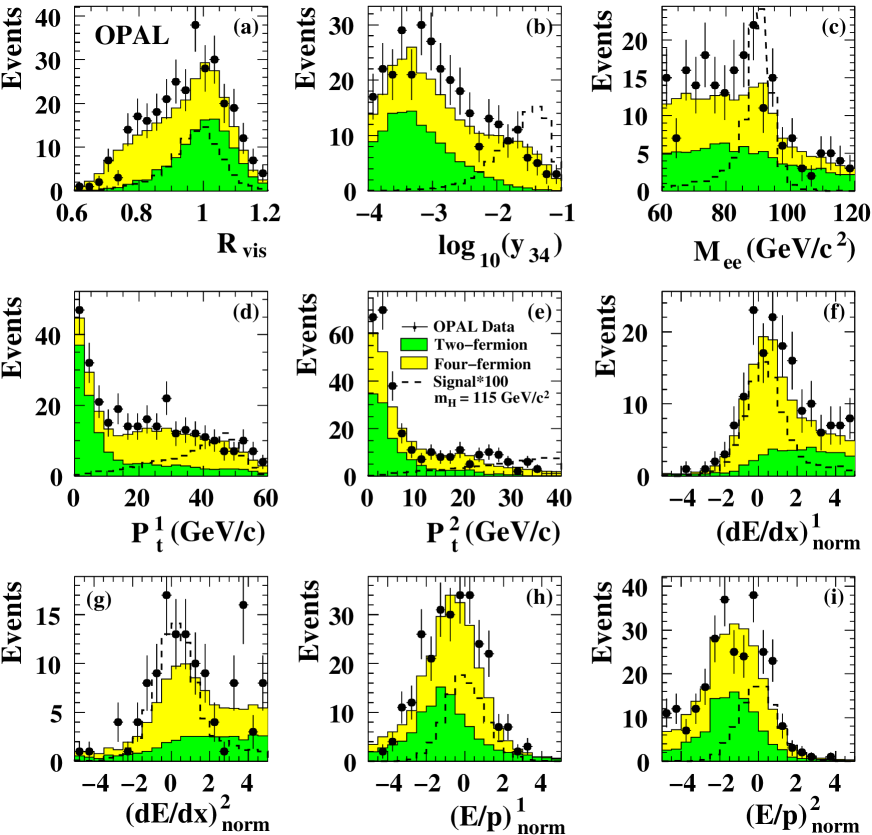
Figure 12: Electron channel: Distributions of the variables used as input to the selection likelihood function. (a) The distribution of the ratio of the visible energy and the energy in the centre-of-mass, (b) $\log_{10}(y_{34})$, (c) the invariant mass of the two electrons, (d) and (e) the transverse momentum of the more and less energetic electron, respectively, (f) and (g) the normalised ionisation energy loss of the more and less energetic electron, (h) and (i) $(E/p)_{\mathrm{norm}}$, of the more and less energetic electron.

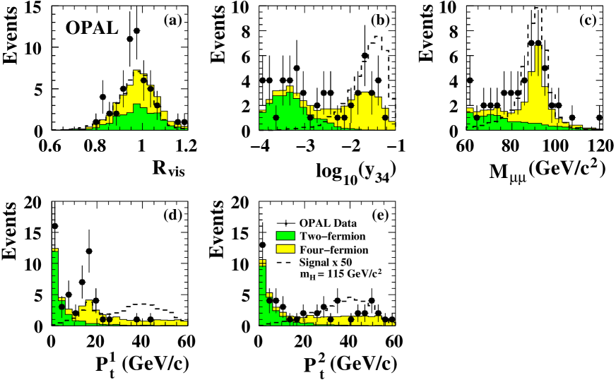
Figure 14: Muon channel: Distributions of the variables used as input to the selection likelihood function. (a) The distribution of the ratio of the visible energy and the energy in the centre-of-mass, (b) $\log_{10}(y_{34})$, (c) the invariant mass of the two muon candidates, (d) and (e) the transverse momentum of the more and less energetic muon, respectively.

The distributions of the input variables to the ${\cal K}$ likelihood are shown in Figure 12 and in Figure 14 for the electron and muon channels, respectively.

The b-flavour requirement, ${\cal B}_{\rm 2jet}$, is the likelihood obtained by combining in one single likelihood the b-probabilities of the two jets. The background is weighted according to the branching fractions for $\mathrm{Z}$ decay since the dominant background arises from $\mathrm{Z}\mathrm{Z}$ production.

The signal likelihood is given by combining ${\cal K}$ and ${\cal B}_{\rm 2jet}$:

$${\cal L}=\frac{{\cal K}\cal B_{\mathrm{2jet}}}{{\cal K}{\cal B}_{\rm 2jet}+(1-{\cal K})(1-{\cal B}_{\rm 2jet})}$$ (3)

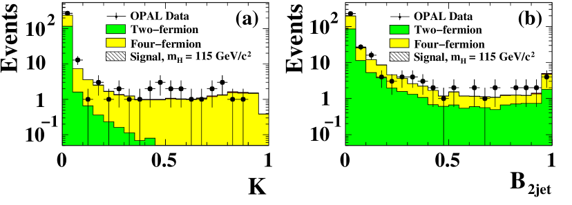
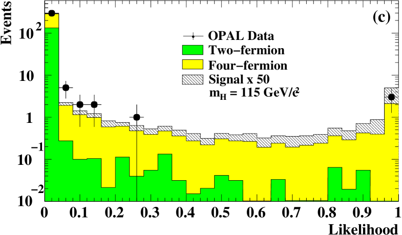
Figure 13: Electron channel: Plots (a), (b) and (c) show the distributions of the ${\cal K}$, ${\cal B}_{\mathrm{2jet}}$ and ${\cal L}$ likelihoods, respectively.

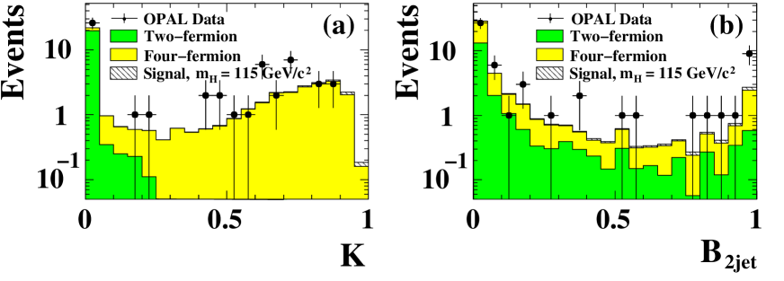
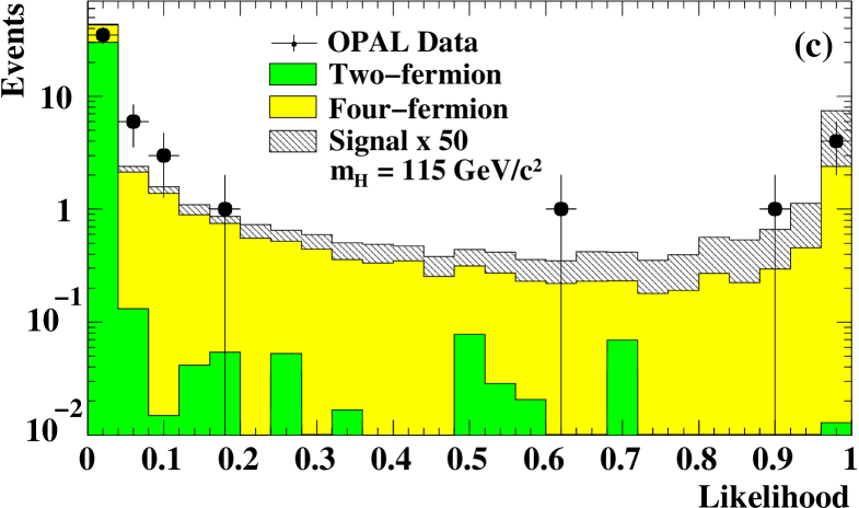
Figure 15: Muon Channel: Plots (a), (b) and (c) show the distribution of the ${\cal K}$, ${\cal B}_{\mathrm{2jet}}$ and ${\cal L}$ likelihoods, respectively.

The distributions of ${\cal L}$ are shown in Figure 13(c) and Figure 15(c) for the electron and muon channels, respectively.

In this channel, the reconstructed Higgs boson mass is used for the mass-dependent part of the discriminator calculation, and the likelihood output ${\cal L}$ is used for the mass-independent part.

Likelihood cuts at 0.2 for the electron channel and 0.3 for the muon channel are introduced for the calculation of systematic errors and for illustration of event rates and distributions in tables and figures. The reconstructed Higgs boson mass $m_{\mathrm{H}}^{\mathrm{rec}}$ is given by the recoil mass to the lepton pair and is shown in Figure 16(d).

The numbers of observed and expected events after each stage of the selection are given in Tables 2 and 3 for the data taken in 1999 and 2000, respectively. The selection retains 4 events in the electron channel, while one expects a background rate of 7.7$\pm$1.4 events. In the muon channel 10 events remain, with an expectation from background of 6.7$\pm$1.0 events.

4.5 Systematic Uncertainties

A large variety of systematic uncertainties have been investigated. Many of them affect both the estimates of the signal efficiencies and those of the background rates. Some of them are shared between decay channels, or between data sets taken at different centre-of-mass energies (for example the modelling of the variables with the same Monte Carlo generators), while others are not. For this reason, the relative signs of the errors as well as their absolute size are relevant in the statistical limit setting procedure discussed in Section 5 below.

The different sources of systematic errors which have been considered are enumerated below and listed, with their relative signs, in Table 4. Note that in the statistical procedure errors from different sources are considered to be uncorrelated.

• Monte Carlo statistics: These uncertainties affect the signal and background rates and are uncorrelated between channels, energies, and signal and background.

The following uncertainties are correlated between all channels and centre-of-mass energies:

• Tracking resolution in $r\phi$: This uncertainty is evaluated with the Monte Carlo simulation by multiplying the discrepancy between the true and reconstructed values of the track’s impact parameter in the $r\phi$ plane, azimuthal angle $\phi$ and curvature by smearing factors of 1.05 and comparing efficiencies to the simulation without extra smearing. The smearing factor 1.05 adequately covers the discrepancies seen in Figure 3(b) and (d).

• Tracking resolution in $z$: This uncertainty is evaluated by treating the track impact parameter in $z$ and $\tan\lambda=\cot\theta$ in the same way as described above, again using smearing factors of 1.05.

• Hit-matching efficiency for $r\phi$-hits in the silicon microvertex detector: One percent of the hits on the $r\phi$ strips of the silicon microvertex detector, which are associated to tracks, are randomly dropped and the tracks are refitted. This uncertainty is chosen positive if the selection rate increases as hits are dropped. The hit dropping fractions were obtained from studies of the $\mathrm{Z}$ calibration data.

• Hit-matching efficiency for $z$-hits in the silicon microvertex detector: This uncertainty is evaluated in the same way as for the $r\phi$ hits, except that 3% of the $z$-hits are dropped.

• B hadron charged decay multiplicity: The average number of charged tracks in B hadron decay is varied within the range recommended by the LEP Electroweak Heavy Flavour Working Group [31], $n_{\mathrm{B}}=4.955\pm 0.062$. The uncertainty is given a positive sign if the selection efficiency increases with the average decay multiplicity.

• B hadron momentum spectrum: The b fragmentation function has been varied so that the mean fraction of the beam energy carried by B hadrons, $\langle x_{E}(\mathrm{b})\rangle$, is varied in the range $0.702\pm 0.008$ [31] using a reweighting technique. The uncertainty is given a positive sign if the selection efficiency rises with increasing average momentum.

• Charm hadron production fractions: The branching ratios of charm hadrons in charm quark decays have been varied within the ranges BR$(\mathrm{c}\mbox{$\rightarrow$}\mathrm{D}^{+})=0.237\pm 0.016$, BR$(\mathrm{c}\mbox{$\rightarrow$}\mathrm{D}_{\mathrm{s}})=0.130\pm 0.027$ and BR $(\mathrm{c}\mbox{$\rightarrow$}\mathrm{c}_{\mathrm{baryon}})=~{}0.096\pm 0.023$ [32]. The uncertainty is given a positive sign if the selection efficiency increases with the charm hadron multiplicity. Each uncertainty is considered individually in the limit calculation, but they are summed in quadrature in Table 4.

• Charm hadron decay multiplicity: The average number of charged and neutral particles in charm hadron decay is varied within the measured ranges [33]. The number of charged particles in $\mathrm{D}^{0},\mathrm{D}^{+}$ and $\mathrm{D}_{\mathrm{s}}$ decays has been varied within $n_{\mathrm{D}^{0}}=2.56\pm 0.05$, $n_{\mathrm{D}^{+}}=2.38\pm 0.06$, $n_{\mathrm{D}_{\mathrm{s}}}=2.69\pm 0.32$, respectively. The number of $\pi^{0}$s in $\mathrm{D}^{0}$ and $\mathrm{D}^{+}$ decays has been varied within the ranges $n_{\mathrm{D}^{0}}=1.31\pm 0.27$, $n_{\mathrm{D}^{+}}=1.18\pm 0.33$, respectively. The uncertainty is given a positive sign if the selection efficiency increases with the average decay multiplicity. Each uncertainty is considered individually in the limit calculation, but they are summed in quadrature in Table 4.

• Charm hadron momentum spectrum: As for the B hadron momentum spectrum, $\langle x_{E}(\mathrm{c})\rangle$ has been varied in the range $0.484\pm 0.008$ [31].

• Comparison of different SM background Monte Carlo generators: Besides the main generators used (see Section 2), the background simulations are cross-checked with alternative generators and fragmentation models such as KORALW [34] and HERWIG [15].

• Four-Fermion production cross-section: This is taken to have a 2% relative uncertainty, arising from the uncertainty in the $\mathrm{Z}\mathrm{Z}$ and $\mathrm{W}^{+}\mathrm{W}^{-}$ cross-sections [35].

The remaining uncertainties are channel dependent and assumed uncorrelated between the channels, but correlated between centre-of-mass energies for the same channel:

• Modelling of likelihood variables: These uncertainties are evaluated by rescaling each input variable in the Monte Carlo individually so as to reproduce the mean and variance of the data. This scaling is done at the level of the preselection cuts and the contributions evaluated for each of the variables are then summed in quadrature.

• Double-ISR rate: For the missing-energy channel, the systematic uncertainty on the background rate includes, in addition to the shared systematic uncertainties, a relative error of 1.24% on the rate of ${\mathrm{e}}^{+}{\mathrm{e}}^{-}$$\rightarrow$$\mathrm{q}\bar{\mathrm{q}}$$\gamma\gamma$ events (“double-ISR”). This systematic uncertainty was evaluated by comparing the selections for $\mathrm{q}\bar{\mathrm{q}}$ background events generated with two different settings of the KK2F generator [11]: one using the Coherent Exclusive EXponentiation (CEEX) matrix elements up to first order and one using up to second order QED corrections, both for initial and final state radiation (FSR). Interference effects between ISR and FSR were neglected in this study.

• Tau identification: In the tau channels the modelling of the fake rates is studied using high-statistics ${\mathrm{e}}^{+}{\mathrm{e}}^{-}$$\rightarrow$$\mathrm{q}\bar{\mathrm{q}}$ data sets taken at $\sqrt{s}\approx\mbox{$m_{\mathrm{Z}}$}$. The modelling of the signal inputs is studied using mixed events which are constructed by overlaying ${\mathrm{e}}^{+}{\mathrm{e}}^{-}$$\rightarrow$$\mathrm{q}\bar{\mathrm{q}}$ events with single hemispheres of ${\mathrm{e}}^{+}{\mathrm{e}}^{-}$$\rightarrow$$\tau^{+}\tau^{-}$ events at $\sqrt{s}\approx\mbox{$m_{\mathrm{Z}}$}$. The systematic error estimated from these studies is $\pm 10\%$ for the single tau fake rate. To be conservative, the error on the single tau efficiency is chosen as the largest of the errors obtained when applying a cut at the tau ANN$>$0.5 and ANN$>$0.75 resulting in a $\pm 3\%$ contribution.

• Electron and muon identification: The estimated contribution accounting for the observed differences between data and Monte Carlo simulation in the lepton identification are estimated to be, together with the contributions from the modelling of the likelihood variables, 1.2% and 8.5% in the electron channel, and 0.5% and 3.5% in the muon channel for signal and background, respectively.

5 Statistical Procedures

The statistical evaluation of the data events which remain after the selection criteria is done in two steps. Firstly all candidate events are classified according to their signal-likeness, and secondly the calculation of confidence levels is made, assuming background-only and signal+background hypotheses. This section describes the procedures used.

5.1 Event Classification

In the four-jet channel only one test-mass dependent discriminating variable is used for the limit calculation, the discriminator function ${\cal{D}}(m_{\mathrm{H}})$, which already incorporates both mass-dependent and mass-independent information. For all the other channels an event classification function is calculated, using the likelihood or ANN value, ${\cal L}$, and the reconstructed Higgs boson mass. Using the two binned distributions directly in the limit calculation is inconvenient due to the large amount of Monte Carlo statistics needed to estimate accurately the expected signal and background in each bin. Furthermore, the histograms must be interpolated between $\sqrt{s}$ and test-mass values where they are evaluated.

A simplification is to form histograms of $m_{\mathrm{H}}^{\mathrm{rec}}$ and ${\cal L}$ in Monte Carlo events, and to smooth them into separate functions for signal and background, $f_{s}(\mbox{$m_{\mathrm{H}}^{\mathrm{rec}}$})$, $f_{b}(\mbox{$m_{\mathrm{H}}^{\mathrm{rec}}$})$, $g_{s}({\cal L})$ and $g_{b}({\cal L})$. These functions are normalised to the expected rates of signal and background, respectively. The event classification function, $W$, is then defined as:

$$W=f_{s}(\mbox{$m_{\mathrm{H}}^{\mathrm{rec}}$})g_{s}({\cal L})/[f_{s}(\mbox{$m_{\mathrm{H}}^{\mathrm{rec}}$})g_{s}({\cal L})+2f_{b}(\mbox{$m_{\mathrm{H}}^{\mathrm{rec}}$})g_{b}({\cal L})].$$ (4)

The values of this function are, by construction, between zero and one. It is chosen so that the separation of the mean values for a background-only and a signal+background scenario, divided by the variance, is maximised.

The Monte Carlo signal and background samples are then used to form histograms of $W$, separately for the signal and background, which are then smoothed. There are signal and background distributions of $W$ for each channel at each centre-of-mass energy at which Monte Carlo was generated, and at each test-mass. The distributions of $W$ are interpolated between neighbouring test-masses and centre-of-mass energies to obtain the distributions used in the limit calculation. The value of $W$ for a candidate event at a particular test-mass is also interpolated between $W$ functions evaluated at nearby centre-of-mass energies and test-masses. The smoothed distributions of $W$ for the signal and background are then binned, and the number of candidates in the data in each bin of $W$ are counted. The estimated signal, $s_{i}$, background, $b_{i}$, and number of candidates, $n_{i}$, in each bin are used in the calculation of confidence levels.

5.2 Confidence Level Calculation

Confidence levels are computed by comparing the observed data configuration to the expectations, for two hypotheses. In the background hypothesis, only the SM background processes contribute to the accepted event rate, while in the signal+background hypothesis the signal from SM Higgs boson production adds to the background. Each assumed Higgs boson mass (test-mass $m_{\mathrm{H}}$) corresponds to a separate signal+background hypothesis.

In order to test the signal+background and background hypotheses optimally with the data, a test statistic is defined which summarises the results of the experiment with expectations of the signal+background and background hypotheses maximally different. An optimal choice [24] is the likelihood ratio of Poisson probabilities.

$$Q=P_{\mathrm{poiss}}(data|signal+background)/P_{\mathrm{poiss}}(data|background),$$ (5)

where

$$P_{\mathrm{poiss}}(data|signal+background)=\prod_{i=1}^{n_{\mathrm{bins}}}\frac{(s_{i}+b_{i})^{n_{i}}e^{-(s_{i}+b_{i})}}{n_{i}!},$$ (6)

and

$$P_{\mathrm{poiss}}(data|background)=\prod_{i=1}^{n_{\mathrm{bins}}}\frac{(b_{i})^{n_{i}}e^{-b_{i}}}{n_{i}!}.$$ (7)

The products runs over all bins of all distributions to be combined. The signal estimation, $s_{i}$, depends on the expected signal cross-section, the decay branching ratios of the Higgs boson, the integrated luminosity and the detection efficiency for the signal. The background estimation, $b_{i}$, depends on the SM background cross-sections, the integrated luminosity, and selection efficiencies. The number of observed events in bin $i$ is $n_{i}$. The test statistic is more conveniently expressed in the logarithmic form

$$-2\ln Q=2\sum_{i=1}^{n_{\mathrm{bins}}}s_{i}-2\sum_{i=1}^{n_{\mathrm{bins}}}n_{i}\ln(1+s_{i}/b_{i}),$$ (8)

which reduces to a sum of event weights, $w=\ln(1+s_{i}/b_{i})$, depending on the local $s_{i}/b_{i}$ for each candidate event observed and on the test-mass.

In this procedure an event-weight is assigned to each event. These weights depend on the test-mass, and are shown for some of the selected candidates in Figure 17(a)-(d). The six candidates with highest event weights ($w=\ln(1+s/b)>$0.1) at $m_{\mathrm{H}}$=115 ${\mathrm{GeV}}/c^{2}$ are listed in Table 5.

To test the consistency of the data with the background hypothesis, the confidence level ${\mathrm{1-CL_{b}}}$ is defined as

$$\mbox{${\mathrm{1-CL_{b}}}$}=P(Q\geq Q_{\mathrm{obs}}|background),$$ (9)

the fraction of experiments in a large ensemble of background-only experiments which would produce results at least as background-like as the observed data.

To test the consistency of the data with the signal+background hypothesis, the confidence level ${\mathrm{CL_{s+b}}}$ is defined as

$$\mbox{${\mathrm{CL_{s+b}}}$}=P(Q\leq Q_{\mathrm{obs}}|signal+background),$$ (10)

the fraction of experiments in a large ensemble of signal+background experiments which would produce results less signal-like than the observed data. By definition a signal+ background hypothesis is excluded at the 95% confidence level if $\mbox{${\mathrm{CL_{s+b}}}$}<0.05$. Statistical downward fluctuations in the background can lead to deficits of observed events which are inconsistent with the expected background and this can cause the signal+background hypothesis to be excluded even if the expected signal is so small that there is little or no experimental sensitivity to it. The confidence level ${\mathrm{CL_{s}}}$ is defined to regulate this behaviour of ${\mathrm{CL_{s+b}}}$:

$$\mbox{${\mathrm{CL_{s}}}$}=\mbox{${\mathrm{CL_{s+b}}}$}/\mbox{${\mathrm{CL_{b}}}$}.$$ (11)

There is some loss of sensitivity by using ${\mathrm{CL_{s}}}$ rather than ${\mathrm{CL_{s+b}}}$, but in no case is a limit more restrictive than the one obtained by using ${\mathrm{CL_{s+b}}}$. We therefore consider a signal hypothesis to be excluded at the 95$\%$ CL if $\mbox{${\mathrm{CL_{s}}}$}<0.05$.

Because all of the $s_{i}$, the $b_{i}$ (in general), and the candidates in each bin depend on the test-mass, ${\mathrm{CL_{b}}}$, ${\mathrm{CL_{s+b}}}$, and ${\mathrm{CL_{s}}}$ all depend on the test mass. The limit on the Higgs boson mass is the smallest test-mass $m_{\mathrm{H}}$ such that $\mbox{${\mathrm{CL_{s}}}$}(\mbox{$m_{\mathrm{H}}$})\geq 0.05$. The sensitivity of the analysis can be expressed by the median ${\mathrm{CL_{s}}}$ in an ensemble of background-only experiments. It is used as the figure of merit to optimise the analyses.

Systematic uncertainties are incorporated into the confidence level calculations by varying and reapplying the signal and background estimations, taking correlations into account, assuming Gaussian-distributed uncertainties.

6 Results

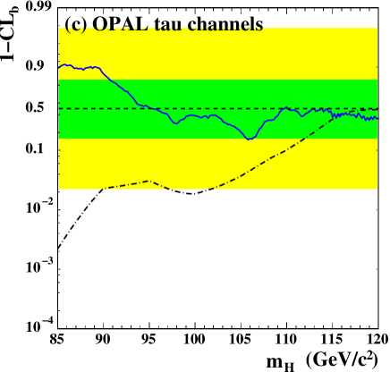
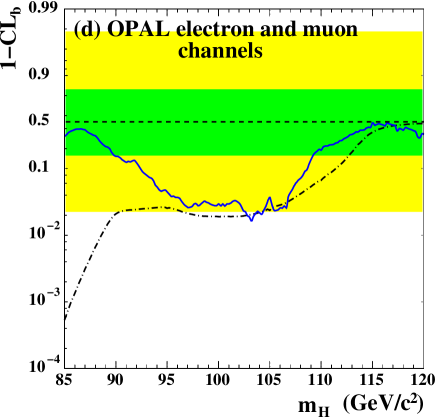
Figure 18: The confidence level $1-$${\mathrm{CL_{b}}}$, as a function of the Higgs boson test-mass, separately for (a) the four-jet channel, (b) the missing-energy channel, (c) the tau channels and (d) the electron and muon channels. The observations for the data are shown with solid lines. The horizontal shaded bands indicate the 68% and 95% probability intervals centred on 0.5, the median expectation in the absence of a signal. The median expectation in the presence of a signal is presented with the dash-dotted line.

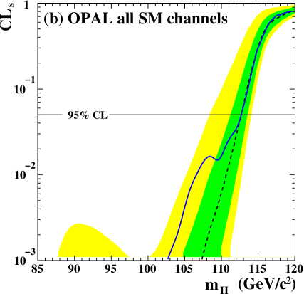
Figure 19: For all search channels combined: (a) The confidence level $1-$${\mathrm{CL_{b}}}$, as a function of the Higgs boson test mass. The median expectation in the presence of a signal is presented with the dash-dotted line. (b) The confidence level ratio ${\mathrm{CL_{s}}}$=${\mathrm{CL_{s+b}}}$/${\mathrm{CL_{b}}}$ versus the Higgs boson test-mass. The observations for the data are shown with solid lines. The shaded bands indicate the 68% and 95% probability intervals, with respect to the median expectation in the absence of a signal (dashed line).

In order to determine the compatibility of the observed data-set with a background-only experiment, the confidence level $1-$${\mathrm{CL_{b}}}$ has been computed as a function of the test-mass $m_{\mathrm{H}}$. The results are shown in Figure 18, along with the distributions expected in an ensemble of background-only experiments and signal+background experiments. If the observed data agreed perfectly with the prediction of the simulated background-only experiment, a value of $1-$${\mathrm{CL_{b}}}$=0.5 would be obtained. A lower (higher) value would indicate an excess (deficit) of data. None of the channels show evidence for a SM Higgs boson. To increase the sensitivity of the search, all channels are combined (Figure 19(a)).

The largest deviation in $1-$${\mathrm{CL_{b}}}$ with respect to the expected SM background is for a Higgs boson mass of 106 ${\mathrm{GeV}}/c^{2}$ with a minimum $1-$${\mathrm{CL_{b}}}$ of about 0.08, which is a much smaller deviation than expected for a Standard Model Higgs boson with a mass of 106 ${\mathrm{GeV}}/c^{2}$.

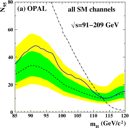
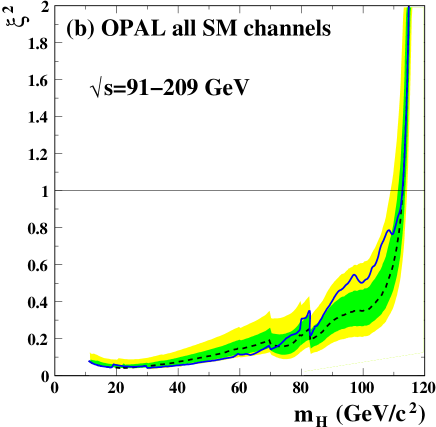
Figure 20: (a) Upper limits on the signal event rate at the 95% confidence level, N₉₅, as observed (solid line) and the expected median (dashed line) for background-only hypotheses, as a function of the Higgs boson test mass. The expected rate of the accepted signal counts for a Standard Model Higgs boson with a mass equal to the test-mass is shown with the dash-dotted line. (b) The 95% CL upper limit on $\xi^{2}$ is shown as a function of the Higgs boson mass $m_{\mathrm{H}}$ as the solid curve. The shaded bands indicate the 68% and 95% probability intervals, with respect to the median expectation in the absence of a signal. For the calculation of N₉₅ and $\xi^{2}$ all available OPAL data with $\sqrt{s}=91-209$ ${\mathrm{GeV}}/c^{2}$ were used.

Also shown in Figure 19(b) is the ${\mathrm{CL_{s}}}$ confidence level, for all search channels combined. The ${\mathrm{CL_{s}}}$ shows the compatibility of the data set with a signal+background hypothesis and also indicates the sensitivity of the search. A signal hypothesis with a ${\mathrm{CL_{s}}}$$\leq$0.05 is considered to be excluded at the 95% confidence level. In this search a Higgs boson mass up to 112.7 ${\mathrm{GeV}}/c^{2}$ is excluded at the 95% CL, with the expected limit from background-only hypotheses also being 112.7 ${\mathrm{GeV}}/c^{2}$. As with other previous OPAL publications [4, 3] no indication of the signal has been found. A comparison between the candidates’ weights $w$ in the previous analysis and in the present paper can be found in Appendix A. Figure 20(a) shows the upper limits on the signal event rate at the 95% CL.

The search results presented here are also used to set 95% CL upper bounds on the square of the HZZ coupling in models which assume the same Higgs boson decay branching ratios as the SM, but in which the HZZ coupling may be different. Figure 20(b) shows the upper bound on $\xi^{2}=(g_{\mathrm{HZZ}}/g_{\mathrm{HZZ}}^{\mathrm{SM}})^{2}$, the square of the ratio of the coupling in such a model to the SM coupling, as a function of the Higgs boson test-mass. In the evaluation of this ratio the $\mathrm{W}^{+}\mathrm{W}^{-}$ and $\mathrm{Z}\mathrm{Z}$ fusion processes are assumed to scale also with $\xi$. The new analyses in the missing energy and four-jet channels are applied starting from $m_{\mathrm{H}}$=80 ${\mathrm{GeV}}/c^{2}$: in Figure 20(b), a discontinuity can be observed corresponding to the transition point both in the expected and the observed curves.

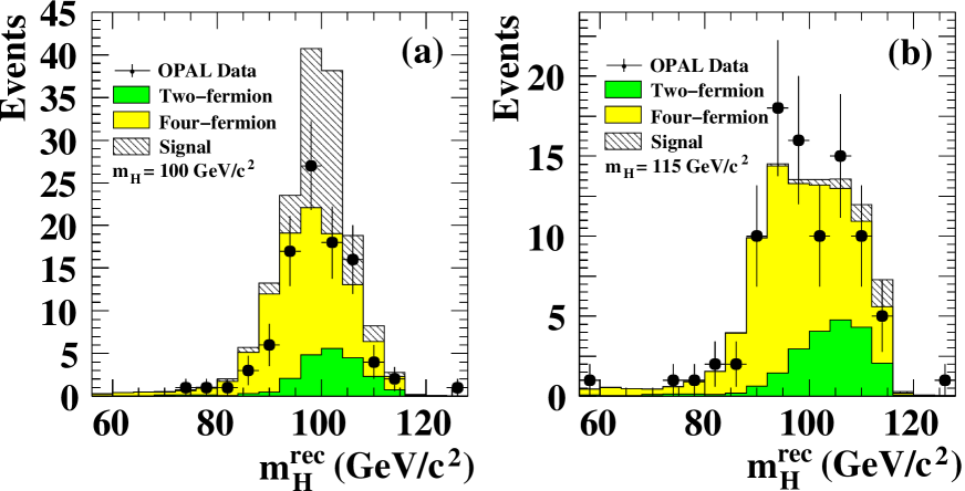
Figure 21: Distributions of the reconstructed mass for the selected events after a cut on the likelihood/ANN for all OPAL channels combined, with the expected contribution (a) from a $m_{\mathrm{H}}$=100 ${\mathrm{GeV}}/c^{2}$ Higgs boson, and (b) from a $m_{\mathrm{H}}$=115 ${\mathrm{GeV}}/c^{2}$ Higgs boson.

The mass distributions for all channels combined, after a cut on the likelihood/ANN value is shown in Figure 21(a) and (b) together with the contribution from a hypothetical SM Higgs boson signal with $m_{\mathrm{H}}$=100 ${\mathrm{GeV}}/c^{2}$ and $m_{\mathrm{H}}$=115 ${\mathrm{GeV}}/c^{2}$, respectively.

7 Summary and Conclusion

A search for the Standard Model Higgs boson has been performed with the OPAL detector at LEP based on the full data sample collected at $\sqrt{s}\approx$192–209 GeV in 1999 and 2000. The largest deviation with respect to the expected SM background in the confidence level for the background hypothesis, $1-$${\mathrm{CL_{b}}}$, is observed for a Higgs boson mass of 106 GeV with a minimum $1-$${\mathrm{CL_{b}}}$ of about 0.08, much less significant than that expected for a Standard Model Higgs boson with a mass of 106 ${\mathrm{GeV}}/c^{2}$. A lower bound of 112.7 ${\mathrm{GeV}}/c^{2}$ on the mass of the SM Higgs boson is obtained at the 95% confidence level for an expected limit from the background-only hypothesis of 112.7 ${\mathrm{GeV}}/c^{2}$. The results do not confirm the excess at $m_{\mathrm{H}}$=115 ${\mathrm{GeV}}/c^{2}$ seen by ALEPH [36], and are similar to the results from L3 [37] and DELPHI [38].

Appendix A Comparison to Previous Published Results

In the four-jet and missing-energy channels new analyses have been developed to improve the sensitivity with respect to the analyses described in Ref. [4]. In each of these channels a comparison between the candidates’ weights $w=\ln(1+s/b)$ in the previous analysis and in the present paper has been performed.

A.1 Four-Jet Channel

The expected sensitivity of the new analysis has been improved over the whole mass range of hypothetical signal masses. For $m_{\mathrm{H}}$=100 ${\mathrm{GeV}}/c^{2}$, $m_{\mathrm{H}}$=110 ${\mathrm{GeV}}/c^{2}$ and $m_{\mathrm{H}}$=115 ${\mathrm{GeV}}/c^{2}$ the improvement of the sensitivity in ${\mathrm{CL_{s}}}$ is about 200%, 32% and 12%, respectively. The comparison of the selected candidates in the four jet channel can be found in Table 6, which contains all events selected by the old analysis with their new weights. The main reasons for changes in the weights are reprocessing of the data, different assignment of the jets to bosons and the treatment of the highest b-tags. The highest b-tags for candidate (16145:37028) changed from 0.595 and 0.251 to 0.344 and 0.219 due to reprocessing. The likelihood value of ${\cal{L_{\mathrm{old}}}}=0.917$ calculated after reprocessing would not have met the old selection criteria of ${\cal{L_{\mathrm{old}}}}>0.96$. Furthermore, the new jet pairing likelihood assigned a different jet pairing to the bosons and the presumed Higgs boson was reconstructed at 88.1 ${\mathrm{GeV}}/c^{2}$. The value of the new discriminating variable for the 115 ${\mathrm{GeV}}/c^{2}$ selection of 0.092 is not high enough to pass the cut value of 0.2. In the case of the three candidates (13978:6299), (15353:24246) and (14847:5404) the jet pairing likelihood assigns the jets with two highest b-tags to different bosons due to kinematical constraints. The old analysis is sensitive only to the two highest b-tags in the event, regardless of the hypothetical boson the jets are assigned to. The new analysis is sensitive to the b-tags of the two jets assigned to the hypothetical Higgs boson.

A.2 Missing-Energy Channel

The expected sensitivity of the new analysis has been improved over the whole mass range of hypothetical signal masses. For $m_{\mathrm{H}}$=100 ${\mathrm{GeV}}/c^{2}$, $m_{\mathrm{H}}$=110 ${\mathrm{GeV}}/c^{2}$ and $m_{\mathrm{H}}$=115 ${\mathrm{GeV}}/c^{2}$ the improvement of the sensitivity in ${\mathrm{CL_{s}}}$ is about 4%, 32% and 8%, respectively. The comparison for the missing-energy channel can be found in Table 7, which contains events with $w\geq 0.05$ for a $m_{\mathrm{H}}$=115 GeV signal in either the new or the old analysis. Only events with $\mathrm{ANN}\geq 0.5$ in the new analysis and likelihood $\geq 0.2$ in the old analysis have been selected. Among the remaining 14 candidates, 11 are selected by both analyses, and 7 out of these have weights larger than 0.05 in both cases. One candidate (15587:18556) is selected by the new analysis only and two are selected by the old analysis only: these two candidates are lost by the new analysis due to the re-processing of the data. Event (15886:54731) fails the preselection having a recoil mass $M_{\mathrm{miss}}$ = 46.3 ${\mathrm{GeV}}/c^{2}$ (the preselection cut is at 50 ${\mathrm{GeV}}/c^{2}$) and event (15648:12732) has a low ANN value of 0.09 since the b-tags of the two jets are low (0.40 and 0.21, respectively) and $M_{\mathrm{miss}}=57.9$ ${\mathrm{GeV}}/c^{2}$.

Table 1: Integrated luminosities of the data samples used for each search channel for the years 1999 and 2000. The differences between search channels are due to different requirements on detector functionality.

	Integrated Luminosity (pb-1)
	Year 1999	Year 2000
Channel	192-202 GeV	200-209 GeV
$\mbox{$\mathrm{H}$}\mbox{$\mathrm{Z}$}\rightarrow\mbox{$\mathrm{b}\bar{\mathrm{b}}$}\mbox{$\mathrm{q}\bar{\mathrm{q}}$}$	217.0	207.3
$\mbox{$\mathrm{H}$}\mbox{$\mathrm{Z}$}\rightarrow\mbox{$\mathrm{b}\bar{\mathrm{b}}$}\mbox{$\nu\bar{\nu}$}$	212.7	207.2
$\mbox{$\mathrm{H}$}\mbox{$\mathrm{Z}$}\rightarrow\mbox{$\mathrm{b}\bar{\mathrm{b}}$}\mbox{$\tau^{+}\tau^{-}$}$/$\tau^{+}\tau^{-}$$\mathrm{q}\bar{\mathrm{q}}$	213.6	203.6
$\mbox{$\mathrm{H}$}\mbox{$\mathrm{Z}$}\rightarrow\mbox{$\mathrm{q}\bar{\mathrm{q}}$}\mbox{${\mathrm{e}}^{+}{\mathrm{e}}^{-}$}$	214.1	203.6
$\mbox{$\mathrm{H}$}\mbox{$\mathrm{Z}$}\rightarrow\mbox{$\mathrm{q}\bar{\mathrm{q}}$}\mbox{$\mu^{+}\mu^{-}$}$	213.6	203.6

Table 2: Cutflow of the selections, applied to the data taken in the year 1999. Number of events after each cut, for the data and for the expected background, normalised to the data luminosity. The two-photon background is not shown separately but is included in the total background. The last column shows the luminosity-weighted average detection efficiencies for a Higgs boson mass of 100 ${\mathrm{GeV}}/c^{2}$, considering $\mathrm{H}$$\rightarrow$$\mathrm{b}\bar{\mathrm{b}}$ in the four-jet channel, $\mathrm{H}$$\rightarrow$all in the missing-energy, electron, and muon channels, and $\mathrm{Z}$$\mathrm{H}$$\rightarrow$$\tau^{+}\tau^{-}$($\mathrm{H}$$\rightarrow$all) or $\mathrm{Z}$$\mathrm{H}$$\rightarrow$$\mathrm{q}\bar{\mathrm{q}}$$\tau^{+}\tau^{-}$ in the tau channel. The number of signal events expected after all cuts are given in parenthesis.

Cut	Data	Total	qq̄($\gamma$)	4-fermi.	Efficiency (%)
		bkg.	bkg.	bkg.	$\mbox{$m_{\mathrm{H}}$}=100$ ${\mathrm{GeV}}/c^{2}$
Four-jet Channel    217.0 pb-1
(1)	20848	20840.9	16232.0	4225.4	99.7
(2)	7251	7217.8	4637.8	2556.1	94.1
(3)	2430	2340.5	580.9	1754.2	87.0
(4)	2413	2309.8	551.8	1752.6	86.9
(5)	2167	2070.0	476.6	1590.8	82.6
(6)	1984	1870.1	408.8	1459.8	79.5
${\cal D}(100)$	30	28.0	7.6	20.4	42.0(12.97$\pm$1.18)
Missing-energy Channel    212.7 pb-1
(1)	5821	5209.5	3290.4	956.7	83.5
(2)	3001	2944.2	2084.3	743.1	74.2
(3)	1534	1506.5	1079.1	414.7	71.9
(4)	625	585.7	258.9	321.6	70.8
(5)	371	358.4	70.1	285.7	65.0
(6)	205	191.8	61.7	130.1	63.1
(7)	152	156.8	34.6	122.2	61.0
${\cal L}^{\mathrm{HZ}}$	10	13.9	2.8	11.1	46.9(5.10$\pm$0.21)
Tau Channel    213.6 pb-1
(1)	5164	5328.3	2992.1	2335.9	78.0
(2)	816	886.1	102.0	784.2	62.4
(3)	207	214.6	55.1	159.6	50.4
(4)	170	186.0	53.8	132.1	50.0
$\cal{L}^{\mathrm{HZ}}$	5	5.1	0.1	5.0	25.8(4.97$\pm$0.23)
Electron Channel 214.1 pb-1
(1)	9560	9656.2	6587.4	3068.8	91.8
(2)	189	158.1	73.9	84.2	75.0
(3)	167	138.0	63.3	74.8	73.8
$\cal{L}^{\mathrm{HZ}}$	3	4.1	0.4	3.8	57.2(0.90$\pm$0.03)
Muon Channel 213.6 pb-1
(1)	9526	9637.0	6574.3	3062.7	87.6
(2)	120	113.2	88.0	25.2	77.1
(3)	26	23.7	10.9	12.8	73.8
$\cal{L}^{\mathrm{HZ}}$	6	3.3	0.0	3.3	62.5(1.08$\pm$0.03)

Table 3: Cutflow of the selections, similar to Table 2, but for the data taken during the year 2000. Efficiencies are given for a hypothetical Higgs boson mass of 115 ${\mathrm{GeV}}/c^{2}$\̇\

Cut	Data	Total	qq̄($\gamma$)	4-fermi.	Efficiency (%)
		bkg.	bkg.	bkg.	$\mbox{$m_{\mathrm{H}}$}=115$ ${\mathrm{GeV}}/c^{2}$
Four-jet Channel    207.3 pb-1
(1)	18242	17990.2	13697.3	4096.6	99.5
(2)	6441	6430.7	3964.7	2456.1	93.2
(3)	2215	2163.8	497.0	1664.2	85.9
(4)	2186	2137.6	472.7	1662.5	85.1
(5)	1982	1912.2	407.6	1503.4	81.3
(6)	1786	1725.9	349.1	1376.0	78.5
${\cal D}(115)$	20	17.5	5.1	12.4	40.0(2.01$\pm$0.18)
Missing-energy Channel    207.2 pb-1
(1)	5417	5059.0	2979.8	1030.1	81.5
(2)	2791	2813.6	1869.8	788.0	73.1
(3)	1463	1515.0	1033.4	444.0	68.6
(4)	595	569.3	230.3	327.4	67.6
(5)	338	351.4	63.3	288.2	58.8
(6)	181	182.8	56.2	126.6	55.5
(7)	154	150.8	31.7	119.2	54.1
${\cal L}^{\mathrm{HZ}}$	11	8.9	2.6	6.3	40.7(1.09$\pm$0.05)
Tau Channel 203.6 pb-1
(1)	4783	4746.7	2476.9	2269.8	78.1
(2)	777	838.8	79.9	758.9	61.2
(3)	190	214.6	43.6	171.0	44.7
(4)	166	168.6	42.2	126.4	43.3
${\cal L}^{\mathrm{HZ}}$	5	4.5	0.2	4.3	25.6(0.26$\pm$0.01)
Electron Channel 203.6 pb-1
(1)	8593	8562.5	5609.3	2953.2	90.9
(2)	169	156.7	69.0	87.7	75.1
(3)	144	137.3	59.3	78.1	73.5
$\cal{L}^{\mathrm{HZ}}$	1	3.6	0.3	3.4	52.9(0.10$\pm$0.003)
Muon Channel 203.6 pb-1
(1)	8452	8441.0	5530.1	2910.9	88.4
(2)	121	109.5	83.3	26.1	76.8
(3)	29	23.3	10.2	13.1	71.8
$\cal{L}^{\mathrm{HZ}}$	4	3.4	0.0	3.4	59.2(0.14$\pm$0.003)

Table 4: Relative systematic uncertainties (in %) on the signal detection efficiencies and background estimations, broken down by source. Negligible sources not studied are denoted with a bar, and non-applicable sources with n/a.

		Channels
Source		$\mathrm{q}\bar{\mathrm{q}}$$\mathrm{H}$	$\nu\bar{\nu}$$\mathrm{H}$	$\tau^{+}\tau^{-}$$\mathrm{q}\bar{\mathrm{q}}$	${\mathrm{e}}^{+}{\mathrm{e}}^{-}$$\mathrm{H}$	$\mu^{+}\mu^{-}$$\mathrm{H}$
Monte Carlo	eff	1.9	1.6	1.9	1.2	1.2
statistics	bkg	5.2	9.5	3.8	4.6	5.4
$r\phi$-	eff	0.7	-0.3	0.7	0.6	-0.6
resolution	bkg	-3.7	1.5	1.3	-2.3	-1.4
$rz$-	eff	0.2	-0.7	0.5	0.3	-0.3
resolution	bkg	-5.4	0.5	0.4	-0.6	-0.9
microvertex $r\phi$	eff	-1.0	0.1	-0.2	0.7	-0.4
hit efficiency	bkg	0.0	2.6	0.2	-4.7	-2.4
microvertex $rz$	eff	-2.5	-0.1	-0.3	0.3	-0.6
hit efficiency	bkg	-0.3	1.3	1.1	-4.7	-2.0
b fragmentation	eff	3.9	0.9	-0.5	1.7	1.6
	bkg	-1.7	2.2	-1.8	0.4	0.6
B decay	eff	0.6	-0.4	0.0	0.1	0.1
multiplicity	bkg	0.5	-0.3	0.1	0.0	0.2
c fragmentation	eff	0.2	0.1	-0.2	0.2	0.1
	bkg	1.2	-0.4	-1.4	0.5	0.5
c hadron	eff	0.7	0.2	-	-	-
fractions	bkg	2.6	0.4	-	-	-
c hadron	eff	3.5	0.2	-	-	-
decay multiplicity	bkg	4.3	1.5	-	-	-
SM MC	eff	n/a	n/a	n/a	n/a	n/a
comparison	bkg	0.4	0.5	4.2	13.8	13.2
Four-fermion	eff	n/a	n/a	n/a	n/a	n/a
cross-section	bkg	1.4	1.5	1.9	1.9	2.0
Channel dependent	eff	6.6	3.6	6.1	1.2	0.5
sources	bkg	11.4	5.1	15.0	8.5	3.5
Total	eff	9.1	4.1	6.5	2.6	2.3
	bkg	15.2	11.7	16.4	18.4	15.3

Table 5: Details for all candidates with an event weight $w=\ln(1+s/b)$ greater than 0.1 at $m_{\mathrm{H}}$=115 ${\mathrm{GeV}}/c^{2}$. In addition to the reconstructed mass, the values of the b-tags for the two jets of the Higgs boson candidate are listed. For the tau channel the value of ${\cal B_{\tau}}$ is presented instead of ${\cal B}_{1}$.

Candidate	$m_{\mathrm{H}}^{\mathrm{rec}}$	Channel	${\cal B}_{1}$	${\cal B}_{2}$	$w_{115}$	$\sqrt{s}$
1	111.2	four-jet	0.94	0.47	0.4342	206.4
2	108.2	missing-energy	0.75	0.24	0.1826	201.7
3	107.2	missing-energy	0.99	0.11	0.1465	201.7
4	112.6	missing-energy	0.31	0.24	0.1333	206.6
5	105.0	tau	0.99	n/a	0.1315	205.2
6	106.6	four-jet	0.98	0.27	0.1295	206.4

Table 6: Four-jet channel: Comparison of $\ln(1+s/b)$-weights for candidates selected by the old analysis, and the weights attributed by the new analysis. A candidate which is not selected in one analysis, is denoted n/s. Events with a weight lower than $10^{-4}$ are listed with zero event-weight. Events indicated in bold are discussed in the text.

			$m_{\mathrm{H}}^{\mathrm{rec}}$		$\ln(1+s/b)$-Weight		$\ln(1+s/b)$-Weight
			GeV		$m_{\mathrm{H}}$=100 GeV		$m_{\mathrm{H}}$=115 GeV
No.	Run:Event		old	new	old	new	old	new
1	16242	8607	78.6	108.6	.1609	.3095	.0424	.0955
2	16221	16299	90.9	91.1	.1742	.1473	.0363	.0302
3	16167	26233	110.5	111.2	1.1286	1.4298	.5324	.4342
4	16145	37028	112.0	n/s	.2381	n/s	.0796	n/s
5	15935	12196	94.6	94.1	.0340	.0000	.0118	.0000
6	15862	19366	107.2	106.8	.6312	.6101	.1135	.1295
7	15821	29240	91.3	90.5	.0402	.0000	.0116	.0000
8	15793	7877	99.6	99.4	.0368	.0835	.0097	.0297
9	15737	30167	107.3	107.1	.3247	.3358	.0584	.0876
10	15705	51066	105.0	50.3	.1344	.0000	.0232	.0000
11	15353	24246	100.6	100.1	.4918	.1092	.1491	.0311
12	15178	17218	90.0	90.7	.1341	.1379	.0405	.0296
13	14847	5404	109.8	109.9	.9444	.1309	.1396	.0203
14	14841	27410	91.0	91.4	.2381	.2825	.0659	.0477
15	14827	32620	92.5	93.2	.1970	.1851	.0424	.0368
16	14729	15555	97.8	97.5	.1627	.0423	.0642	.0138
17	14560	24515	56.1	57.0	.1536	.0000	.0626	.0000
18	14383	14394	98.8	99.2	.2069	.0507	.0821	.0186
19	14268	24264	97.8	97.0	.0342	.0000	.0097	.0130
20	14226	8270	100.7	102.1	.0845	.0610	.0182	.0130
21	14134	74857	0.0	61.2	.1536	.0333	.0626	.0212
22	14022	14470	94.1	94.7	.0269	.0000	.0082	.0000
23	13978	6299	112.6	112.8	.7774	.2375	.4007	.0441
24	13838	4447	100.5	102.1	.0758	.0230	.0167	.0054
25	13275	9526	98.6	98.5	.1667	.2170	.0434	.0790
26	13243	8535	89.7	89.2	.0572	.0641	.0099	.0069
27	12972	10136	59.5	58.9	.1054	.1326	.0088	.0249

Table 7: Same as for Table 6, for the missing-energy channel.

			$m_{\mathrm{H}}^{\mathrm{rec}}$		$\ln(1+s/b)$-Weight		$\ln(1+s/b)$-Weight
			GeV		$m_{\mathrm{H}}$=100 GeV		$m_{\mathrm{H}}$=115 GeV
No.	Run:Event		old	new	old	new	old	new
1	15886	54731	112.1	111.9	.4025	n/s	.2044	n/s
2	15761	28847	110.5	110.3	.2986	.1387	.0707	.0298
3	15648	12732	111.7	111.8	.2234	n/s	.0940	n/s
4	15587	18556	100.7	109.0	n/s	.2295	n/s	.0579
5	15498	13971	112.8	100.4	.1387	.0820	.0571	.0283
6	15429	16226	99.2	112.6	.1648	.2173	.1455	.1333
7	15258	12168	99.1	99.0	.1453	.0998	.0769	.0350
8	15204	40272	104.0	99.3	.3071	.0528	.1224	.0233
9	15178	44741	110.1	105.1	.6734	.2672	.2518	.0908
10	15099	25825	101.8	109.9	.2694	.2173	.0571	.0579
11	14979	16964	108.2	101.6	.3641	.2419	.1551	.0968
12	14383	22908	108.2	108.1	.5871	.3535	.1455	.0968
13	12357	26618	106.9	108.2	.5423	.7580	.0536	.1826
14	12323	12944	107.2	107.2	.5423	.5290	.1456	.1465

Figure 1: Feynman diagrams for (a) the Higgs-strahlung process, (b) the $\mathrm{W}^{+}\mathrm{W}^{-}$fusion process and (c) the $\mathrm{Z}\mathrm{Z}$ fusion process for the production of Higgs bosons in ${\mathrm{e}}^{+}{\mathrm{e}}^{-}$ collisions.

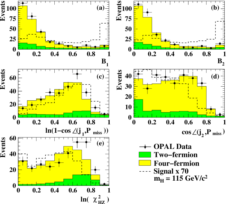
Figure 8: Missing-Energy Channel: Continuation of Figure 7. (a) and (b) the b-tag likelihood output of the more and less energetic jets, (c) the logarithm of $(1-\cos\angle(j_{1},p_{\mathrm{miss}}))$, (d) $\cos\angle(j_{2},P_{\mathrm{miss}})$, (e) the logarithm of $\chi^{2}_{\mathrm{ZH}}$.

Figure 17: Distributions of event weights, $\ln(1+s/b)$, as a function of the Higgs boson test-mass, (a) the four-jet channel, (b) the missing-energy channel, (c) the tau channels, and (d) the electron and muon channels. The discontinuities observed in the case of the missing-energy channel at $\mbox{$m_{\mathrm{H}}$}=107$ ${\mathrm{GeV}}/c^{2}$ are due to the switching between the two ANN’s, trained for low and high mass signals.

References

-
[1]
S. Glashow, Nucl. Phys. 22 (1961) 579;
S. Weinberg, Phys. Rev. Lett. 19 (1967) 1264;
A. Salam, ed. N. Svartholm, Elementary Particle Theory, Almquist and Wiksells, Stockholm (1968) 367. -
[2]
P.W. Higgs, Phys. Lett. 12 (1964) 132;
F. Englert and R. Brout, Phys. Rev. Lett. 13 (1964) 321;
G.S. Guralnik, C.R. Hagen, and T.W.B. Kibble, Phys. Rev. Lett. 13 (1964) 585. - [3] The OPAL Collaboration, G. Abbiendi et. al., Eur. Phys. J. C12 (2000) 567-586.
- [4] The OPAL Collaboration, G. Abbiendi et. al., Phys. Lett. B499 (2001) 38.
- [5] S. Anderson et al., Nucl. Instr. and Meth. A403 (1998) 326.
- [6] The OPAL Collaboration, K. Ahmet et al., Nucl. Instr. and Meth. A305 (1991) 275.
- [7] G. Aguillon et. al., Nucl. Instr. and Meth. A417 (1998) 266.
- [8] G. Abbiendi et. al., Eur. Phys. J. C14 (2000) 373.
- [9] The OPAL Collaboration, K. Ackerstaff et al., Phys. Lett. B391 (1997) 221.
- [10] P. Janot, Physics at LEP2, CERN 96-01, Vol.2, 309.
- [11] S. Jadach, B. F. Ward and Z. W s, Comput. Phys. Commun. 130 (2000) 260.
-
[12]
J. Fujimoto et al., Comp. Phys. Comm. 100 (1997) 128.
J. Fujimoto et al., Physics at LEP2, CERN 96-01, Vol.2, 30. - [13] S. Jadach, W. Płaczek, and B.F.L. Ward, Physics at LEP2, CERN 96-01, Vol.2, 286; UTHEP-95-1001.
-
[14]
E. Budinov et al., Physics at LEP2,
CERN 96-01, Vol.2, 216;
R. Engel and J. Ranft, Phys. Rev. D54 (1996) 4244. - [15] G. Marchesini et al., Comp. Phys. Comm. 67 (1992) 465.
- [16] J.A.M. Vermaseren, Nucl. Phys. B229 (1983) 347.
-
[17]
T. Sjöstrand, Comp. Phys. Comm. 82 (1994) 74;
T. Sjöstrand, LU TP 95-20. - [18] J. Allison et al., Nucl. Instr. and Meth. A317 (1992) 47.
-
[19]
N. Brown and W.J. Stirling, Phys. Lett. B252 (1990) 657;
S. Bethke, Z. Kunszt, D. Soper and W.J. Stirling, Nucl. Phys. B370 (1992) 310;
S. Catani et al., Phys. Lett. B269 (1991) 432;
N. Brown and W.J. Stirling, Z. Phys. C53 (1992) 629. - [20] The OPAL Collaboration, G. Alexander et al., Z. Phys. C70 (1996) 357.
- [21] The OPAL Collaboration, G. Abbiendi et al., Eur. Phys. J. C7 (1999) 407.
-
[22]