Multiplicities, fluctuations and correlations

Abstract

The recent results on hadron multiplicities in heavy and light quark fragmentation, multiplicity local fluctuations and multiparticle correlations submitted to the Conference are reviewed.

1 Introduction

One of the most important observables in particle production processes is multiplicity, i.e. the number of particles (mostly, hadrons) produced in the collision [1]. The multiplicity dependence on the energy scale, species of particles, event flavour content are among the main predictions of the theory of strong interactions, quantum chromodynamics (QCD) [1, 2]. On the other hand, the multiplicity is used to select or to describe events, e.g. as a trigger for specific processes, as an input for kinematic variables’ spectra. The distribution of multiplicity, its mean value and multiplicity fluctuations are the essential characteristics of the collision dynamics. However, the multiplicity distribution tells us just about the averaged, integrated numbers, while deeper information comes from the moments of the distribution, which measure particle correlations, i.e. probe the interaction dynamics [3].

Here, I report on the multiplicity flavour dependence, on the analyses of local multiplicity fluctuations and multiparticle correlations. These studies provide us with details of strong interactions and allow us to estimate the level of the applicability of QCD, based on the partonic picture, to the production of hadrons which are the experimentally observed objects.

2 Definitions and notations [1, 3]

The multiplicity distribution, or the density $\rho_{n}$, of multiplicity $n$ of particles with kinematic variables $p_{1},p_{2},\ldots,p_{n}$ is defined by the inclusive probability spectrum,

$$\rho_{n}(p_{1},p_{2},\ldots,p_{n})=\frac{1}{N_{\rm ev}}\,\frac{dn(p_{1},p_{2},\ldots,p_{n})}{dp_{1}dp_{2}\cdots dp_{n}}\>,$$

where $N_{\rm ev}$ is the number of events.

As it follows from this formula, the single particle distribution $\rho_{1}(p_{1})$ gives an average multiplicity, $\langle n\rangle=\int\rho_{1}(p_{1})dp_{1}$, while integration of the $q$-particle densities leads to the unnormalised $q$th order factorial moments,

$$f_{q}=\int\rho_{1}(p_{1},p_{2}\ldots p_{n})dp_{1}dp_{2}\cdots dp_{n}\vspace*{-.075cm}$$

(1)

$$=\langle n(n-1)\cdots(n-q+1)\rangle\equiv\langle n^{[q]}\rangle\>.$$

The normalised factorial moments are then defined as $F_{q}=f_{q}/\langle n\rangle^{q}$.

The $q$-particle densities give us a way to study particle correlations described by the $q$-particle correlation functions, (factorial) cumulants, $C_{q}(p_{1},\ldots,p_{q})$. The cumulants vanish whenever one of their arguments is statistically independent, i.e. these functions measure genuine $q$-particle correlations.

The cumulants are constructed from the multiplicity densities, e.g.

$$C_{1}(p_{1})=\rho_{1}(p_{1}),$$

$$C_{2}(p_{1},p_{2})=\rho_{2}(p_{1},p_{2})-\rho_{1}(p_{1})\rho_{1}(p_{2}),$$

$$C_{3}(p_{1},p_{2},p_{3})=\rho_{3}(p_{1},p_{2},p_{3})-$$

$$\hskip 4.26773pt\sum_{(3)}\rho_{1}(p_{1})\rho_{2}(p_{2},p_{3})+2\rho_{1}(p_{1})\rho_{1}(p_{2})\rho_{1}(p_{3})\>.$$ (2)

These functions, being properly normalised, are used to study multiparticle correlations in different kinematic variables.

In studies of local fluctuations and correlations, i.e those in phase-space bins, one uses the bin-averaged factorial moments and cumulants. The phase space is divided into $M$ bins of equal size, so that $\langle n_{m}\rangle$ is the number of particles in the $m$th bin. Then, the normalised bin-averaged factorial moment is defined via Eq. (1) averaged over bins,

$$\hskip 5.69046ptF_{q}(M)={1\over M}\sum_{m=1}^{M}\frac{f_{q}(m)}{\langle n_{m}\rangle^{q}}\equiv{1\over M}\sum_{m=1}^{M}\frac{\langle n_{m}^{[q]}\rangle}{\langle n_{m}\rangle^{q}}.$$ (3)

These factorial moments have been extensively used to extract the non-statistical (non-Poissonian) fluctuations in many types of collisions [3]. Such fluctuations lead to the power-law scaling of factorial moments as a function of $M$ called the intermittency phenomenon.

In analogy with Eq. (3), Eqs. (2) are averaged to the bin-averaged normalised cumulants,

$$\hskip 48.36958ptK_{q}(M)={1\over M}\sum_{m=1}^{M}\frac{\langle k_{q}^{(m)}\rangle}{\langle n_{m}\rangle^{q}},$$ (4)

where $k_{q}^{(m)}$ are the Mueller moments, the functions of unnormalised moments $f_{q}(m)$, Eq. (1),

$$k_{1}=\langle n_{m}\rangle,\quad k_{2}^{(m)}=\langle n_{m}^{[2]}\rangle-\langle n_{m}\rangle^{2},$$

$$\hskip 21.33955ptk_{3}^{(m)}=\langle n_{m}^{[3]}\rangle-3\,\langle n_{m}^{[2]}\rangle\langle n_{m}\rangle\,+2\,\langle n_{m}\rangle^{3}.$$ (5)

3 Hadronisation of heavy and light quarks

In this Section, I consider the recent results on hadron multiplicities from fragmentation of heavy and light quarks [6, 7, 8]. The study of the quark content in multiparticle production provides one of the basic tests of QCD. The results from LEP are of a special interest since they cover a wide centre-of-mass energy region and can be directly compared with QCD which is mostly predictable at the asymptotic energies [2].

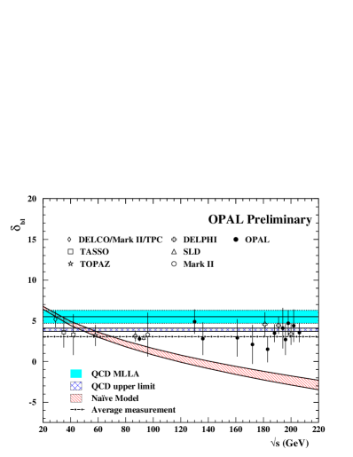
Figure 1: The difference in the mean charged multiplicities, $\delta_{\rm bl}$, between heavy and light quark pairs as a function of centre-of-mass energy. The dashed-dotted line is the combined result from all measurements, see Ref. [8] for more details.

In Refs. [6] and [8], a study of the fragmentation of heavy b-quark and light quarks (l = u, d, s) is performed. The measurements of the difference in charge particle multiplicities, $\delta_{\rm bl}=\langle n_{{\rm b}{\bar{\rm b}}}\rangle-\langle n_{{\rm l}{\bar{\rm l}}}\rangle$, for ${\rm b}{\bar{\rm b}}$ and ${\rm l}{\bar{\rm l}}$ events in e⁺e^- annihilation at the centre-of-mass energies above the Z⁰ peak are carried out. The findings are compared to the theoretical predictions of QCD and to a more phenomenological (the so-called naïve) model (for review, see Ref. [2]). The QCD calculations predict energy-independent behaviour of the multiplicity difference $\delta_{\rm bl}$, while in the naïve model one expects the decrease with increasing energy. The latter is connected with the assumption that the hadron multiplicity accompanying the heavy hadrons in ${\rm b}{\bar{\rm b}}$ events is the same as the multiplicity in ${\rm l}{\bar{\rm l}}$ events at the energy left to the system once the heavy quarks have fragmented.

The difference between the heavy and light mean quark-pair multiplicities obtained by DELPHI at 206 GeV is $\delta_{\rm bl}=4.50\pm 1.05({\rm stat})\pm 0.52({\rm syst})$ [8], while OPAL finds $\delta_{\rm bl}=3.44\pm 0.40({\rm stat})\pm 0.79({\rm syst})$ in the energy range of 130 – 206 GeV [8]. The difference in the values is connected with some differences in the data processing procedure. In the meantime, the results of the energy-dependence is found to be the same for the both studies: the mean multiplicity difference is energy-independent and favours the QCD predictions while it is inconsistent with the flavour-independent naïve model (Fig. 1). Also in agreement with QCD is the ratio between light quark multiplicities, $\langle n_{\rm i}\rangle:\langle n_{\rm j}\rangle\sim 1$, where i,j ={u,d,s}, as obtained by OPAL at the Z⁰ peak energy [7]. To note is that the $\langle n_{\rm u}\rangle$ and $\langle n_{\rm d}\rangle$ are highly statistically anti-correlated ($-90$%) which is due to their fractions in K-mesons.

4 Scaling of local fluctuations in hadronic Z⁰ decays

During the last decades, the phase-space local multiplicity fluctuations are actively studied in many reactions, from leptonic to nuclear collisions, and the intermittency scaling of the fluctuations has been established [3].

All the studies show that the intermittency is more pronounced in high dimensions, while in one dimension (e.g., in rapidity) the effect is diluted by projection onto one dimension. This leads to flattenning of the factorial moments. Such a behaviour is well understood from a QCD parton shower which is a three-dimensional branching and naturally leads to the fractality. The best area to study the effect and its connection with QCD is given by e⁺e^- annihilation, where such investigations has been performed earlier [3, 9, 10] and new analysis is carried out by L3 [11].

The L3 analysis gives us further hints about the intermittency origin, which is currently far from understanding. The new study employs the fact that so far the fluctuations in many dimensions were studied with the same number $M$ of bins in each dimension/direction. This leads to self-similar fractals, i.e. the fluctuations in any direction are assumed to be the same, or isotropic. In case when the dynamics in different directions are not equivalent, the fluctuations become anisotropic and this tells us about the self-affinity [12]. A self-affine behaviour has been observed in hadronic interactions [12], while a self-similar scaling has been qualitatively confirmed in e⁺e^- annihilation [10]. In terms of factorial moments, Eq.(3), the 3-dimensional moments are expected to exhibit the intermittency property in e⁺e^- collisions when phase-space is partitioned isotropically, while this scaling in hadronic interactions only occurs for anisotropic partitioning.

Figure 2: The 1-dimensional 2nd-order factorial moments, Eq. (3), as a function of the number $M$ of bins in the randomised and the thrust frames compared to the Monte Carlo predictions with and without Bose-Einstein correlations. The fit is given by the first f-la of Eqs. (7). The behaviour in the q${\bar{\rm q}}$ frame is similar to that in the randomised frame. See text and [11] for details.

In order to quantitatively study the observed isotropic fluctuations, the method of the Hurst exponent is used [12]. The Hurst exponent,

$$\hskip 56.9055ptH_{ab}={\ln M_{a}}/\,{\ln M_{b}},$$ (6)

is obtained from the fit of the one-dimensional second-order factorial moments,

$$F_{2}(M_{a})=A_{a}+B_{a}\,M_{a}^{-\gamma_{a}}\>\Rightarrow\>H_{ab}=\frac{1+\gamma_{b}}{1+\gamma_{a}}.$$ (7)

Here $a$, $b$ are the directions of the $(a,b)$ plane. For the isotropic dynamical fluctuations, $H_{ab}=1$, while $H_{ab}\neq 1$ if the fluctuations are anisotropic.

L3 uses rapidity $y$, azimuthal angle $\varphi$ and transverse momentum $p_{t}$ – the variables often used in multiparticle studies – in the analysis. The variables are defined with respect to the thrust axis, as well as the other two frames are considered: the randomised and the q${\bar{\rm q}}$ frames. In the former one, the $\varphi$-angles are randomly chosen being uniformly distributed in $[0,2\pi]$, while in the latter case one uses Monte Carlo to correct the original thrust axis to the q${\bar{\rm q}}$ axis.

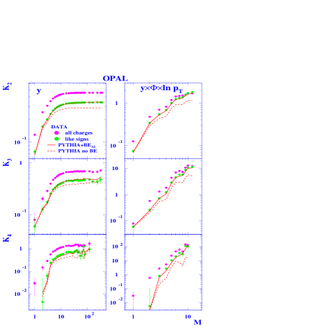
Figure 3: The all-charge and like-sign cumulants, Eq. (4), as a function of the number $M$ of bins in rapidity and in three dimensions. The like-sign cumulants are compared to the Monte Carlo predictions with and without Bose-Einstein correlations. See text and Ref. [13] for more details.

The 3-dimensional factorial moments are found to exhibit the intermittency scaling when phase-space is isotropically partitioned. This confirms earlier indications for isotropic fluctuations in e⁺e^- annihilations [9, 10]. No sensitive differences in the different frames as well as no disagreements between the data and Monte Carlos are observed.

Fig. 2 shows the 2nd-order factorial moments in one dimension, from which the quantitative test of the isotropy of the fluctuations is made using Eqs. (7). The calculations of the Hurst exponent give: $H_{ab}\approx 1$, $a,b=\{y,\varphi,p_{t}\}$, i.e. due to the definition of Eq. (6) one concludes about the equivalence of the directions and about the isotropy of the fluctuations. The fluctuations in $\varphi$ are nearly absent in the thrust frame. In all frames the data are well described by Jetset, while somewhat less well by Herwig. No sensitivity to Bose-Einstein correlations is seen. From its study, L3 also concludes that there is the dependence on the QCD dynamics which serves to decrease the fluctuations in the thrust frame.

The 2-jet sub-samples are also analysed using the Durham jet algorithm. The fluctuations in the 2-jet events show the self-affine (anisotropic) fluctuations. This looks like the hard gluon emission leads to the isotropy.

5 Multiparticle correlations

The multiparticle correlation studies are performed for e⁺e^- annihilations at the Z⁰ energy [13] and for ${\bar{\rm p}}$p annihilation at the incident momentum of 22.4 GeV/$c$ [14].

Genuine multiparticle correlations in e⁺e^- annihilations are studied by OPAL [13]. To extract the correlations, the method of the bin-averaged normalised cumulants is used, see Eqs. (4)–(5). In addition to the earlier analysis [10] of the cumulants of all charged particles (“all-charge cumulants”), OPAL studies the cumulants of same-charge particles (“like-sign cumulants”). The investigation is performed in rapidity $y$, azimuthal angle $\varphi$ and transverse momentum $p_{t}$, the same variables as in the above described L3 analysis, but the sphericity axis is used as a reference axis.

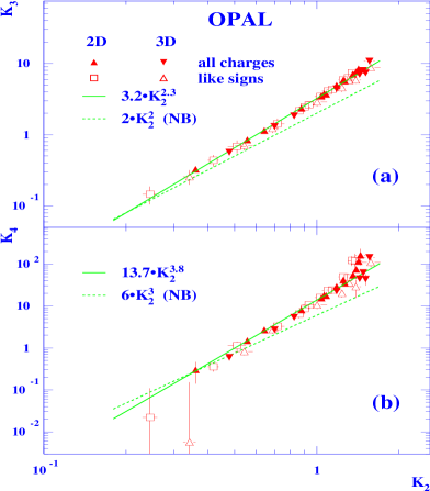
Figure 4: The Ochs-Wosiek plot in two and three dimensions for all-charge and like-sign cumulants. The dashed line shows the Negative Binomial prediction. The solid line is a fit, $\ln K_{q}=a_{q}+r_{q}\ln K_{2}$. See text and [13] for more details.

Fig. 3 shows the all-charge and like-sign cumulants calculated in one (rapidity) and three dimensions. Even in one dimension, positive genuine correlations of groups of two, three, four particles are present. The cumulants exhibit a scaling behaviour, although in rapidity the saturation already appears at the moderate bin sizes. The like-sign cumulants increase faster and drive the all-charge ones at small bins while the unlike-sign cumulants are almost constant. This points to the likely influence of Bose-Einstein correlations.

The comparison between the data and Monte Carlo like-sign cumulants shows that the model describes well the data when Bose-Einstein correlations are implemented. The same is true for the all-charge cumulants (not shown here). This is not the case of the L3 results where no difference is found for the models with and without Bose-Einstein correlations, see Fig. 2. To note is that the OPAL data is described well in one dimension as well as in three dimensions.

From Fig. 3, one can see that Bose-Einstein correlations which are implemented in the model as the correlations of two identical particles and are pair-wise adjusted, well also describe the cumulants of $q>2$. This suggests to consider the interdependence of the 2nd- and higher-order cumulants, Fig. 4. The fit akin to the Ochs-Wosiek one [3] gives the same parameter values for the all-charge and like-sign cumulants, while disagrees with the Negative Binomial predictions.

The multiparticle fluctuations are also studied in [14] using the Serpukhov fixed target ${\bar{\rm p}}$p annihilation data at 22.4 GeV/$c$. The differential spectra of $k$ particles in pseudorapidity bins are analysed relative to the similar background spectra. The dips in the distributions of such ratios are found to be independent on the number $k$ of particles, $\sim 1.8$. The number of clusters is estimated to be about 2-3 with two particles per cluster in average. It is found that the data in the non-annihilation channel is similar to that from the inelastic pp collisions at 69 GeV/$c$ from the same accelerator. These observations are treated in frames of different mechanisms, e.g. a model with mesons emitted from intermediate nucleon isobars is suggested.

I am thankful to the ICHEP02 Organising Committee, to convenors of the QCD Session, and to my colleagues at CERN and particularly in OPAL for giving me the opportunity to make this presentation and for their kind help and support.

References

- [1] I.M. Dremin, J.W. Gary, Phys. Rep. 349 (2001) 301.
- [2] V.A. Khoze, W. Ochs, Int. J. Mod. Phys. A12 (1997) 2949.
- [3] E.A. De Wolf, I.M. Dremin, W. Kittel, Phys. Rep. 270 (1996) 1.
- [4] M. Siebel, Fragmentation of quarks and gluons, these Proceedings.
- [5] Š. Todorova-Nová, Bose-Einstein correlations at LEP and HERA, these Proceedings.
-
[6]
P. Abreu, A. De Angelis, DELPHI 2002-052 CONF 586 (2002), ICHEP02 abs.
232;
DELPHI Collaboration, P. Abreu et al., Phys. Lett. B479 (2000) 118. - [7] OPAL Collaboration, G. Abbiendi et al., Eur. Phys. J. C19 (2001) 257.
- [8] OPAL Collaboration, Physics Note PN511 (2002), ICHEP02 abs. 373.
- [9] DELPHI Collaboration, P. Abreu et al., Nucl. Phys. B386 (1992) 471.
- [10] OPAL Collaboration, G. Abbiendi et al., Eur. Phys. J. C11 (1999) 239.
- [11] L3 Collaboration, L3 Note 2758 (2002), ICHEP02 abs. 494.
- [12] Liu Feng, Liu Fuming, Liu Lianshou, Phys. Rev. D59 (1999) 114020 and refs. therein.
- [13] OPAL Collaboration, G. Abbiendi et al., Phys. Lett. B523 (2001)35, ICHEP02 abs.319.
- [14] E.G. Boos et al., ICHEP02 abs. 37.