CompAZ: parametrization of the luminosity spectra for the photon collider.

Abstract

A simple model, based on the analytical formula for the Compton scattering, is proposed to describe the realistic photon-energy spectra for the Photon Collider at TESLA. Parameters of the model are obtained from the full simulation of the beam by V.Telnov, which includes nonlinear corrections and contributions of higher order processes. Photon energy distribution and polarization, in the high energy part of the spectra, are well reproduced. Our model can be used for a Monte Carlo simulation of gamma-gamma events at various energies and for direct cross-section calculations.

1 Introduction

Photon Collider has been proposed as a natural extension of the $e^{+}e^{-}$ linear collider project TESLA [1]. High-energy photons can be obtained using Compton backscattering of the laser light off the high-energy electrons [2, 3, 4, 5, 6]. The physics potential of the Photon Collider is very rich and complementary to the physics program of $e^{+}e^{-}$ and hadron colliders [1]. It is the ideal place to study the mechanism of the electroweak symmetry breaking (EWSB) and properties of the Higgs boson. Precision measurements at the Photon Collider may open “new windows” to the physics beyond the Standard Model. However, the precise measurements are only possible if the energy spectrum of colliding photons is well understood. A detailed simulation of the $\gamma\gamma$  luminosity spectra at the Photon Collider at TESLA has become available recently [6, 7]. In this paper a simple model based on these results is proposed.

2 Luminosity spectra

If the laser beam density is small and the primary electron beams are sufficiently wide, so that effects related to the photon scattering angle can be neglected, the energy spectrum of the photon beams colliding in the Photon Collider could be calculated directly from the Compton scattering cross section (see appendix A). However, these assumptions will not be fulfilled at the Photon Collider as we need both very powerful lasers and strongly focused electron beams to get high luminosity. To find the energy spectra of colliding photons, with realistic assumptions about the laser system and the electron beams, detailed simulation programs has been prepared [6, 8].

New samples, with high statistics of the simulated $\gamma\gamma$ events, have been generated recently by V.Telnov [7]. They are based on the beam and laser system layout and parameters, as proposed for the Photon Collider at TESLA [1]. Electron beam energies of 100, 250 and 400 GeV have been considered. Basic parameters used in the simulation are listed in Table 1. More details of the simulation can be found in [1, 7, 9].

$E_{e}$ [GeV]	100	250	400
$\lambda_{L}$ [$\mu m$]	1.06	1.06	1.06
$E_{0}$ [eV]	1.17	1.17	1.17
$x$	$1.8$	$4.5$	$7.2$
$\sigma_{x}$ [nm]	140	88	69
$\sigma_{y}$ [nm]	6.8	4.3	3.4
$\sigma_{z}$ [mm]	0.3	0.3	0.3
$f_{rep}$ [kHz]	14.1	14.1	14.1
$\gamma\epsilon_{x/y}/10^{-6}$ [m$\cdot$rad]	2.5/0.03	2.5/0.03	2.5/0.03
$\beta_{x/y}$ [mm] at IP	1.5/0.3	1.5/0.3	1.5/0.3
b [mm]	2.6	2.1	2.7
$L_{ee}\,(geom)$ [$10^{34}\,cm^{-2}s^{-1}$]	4.8	12	19

Table 1: Parameters of the Photon Collider based on TESLA. Listed for different electron beam energies $E_{e}$ are: laser wave length $\lambda_{L}$, laser photon energy $E_{0}$ and resulting $x$ parameter values (see section 3 and appendix A); horizontal, vertical and longitudinal electron bunch sizes $\sigma_{x}$, $\sigma_{y}$ and $\sigma_{z}$; average repetition rate, normalized beam emittances $\gamma\epsilon_{x/y}$, $\beta$-functions $\beta_{x/y}$ , distance between the conversion and interaction point and estimated $e^{-}e^{-}$ luminosity.

Shown in Fig. 1 are the distribution of the colliding photon energy ratio to the primary electron beam energy, $y=E_{\gamma}/E_{e}$, and the distribution of the $\gamma\gamma$ center-of-mass energy distribution, $W_{\gamma\gamma}$. Results obtained from the simulation of luminosity spectrum [7], for electron beam energy of 250 GeV, are compared with the distributions expected from the simple Compton scattering (lowest order QED), as given by formula (14) (see appendix A). Realistic simulation indicates that a large fraction of colliding photons will have small energies. Also the maximum of the high-energy peak is shifted towards lower energies.

Shown in Fig. 2 (left plot) is the two-dimensional energy distribution for the colliding photons, as obtained from the simulation [7], for electron beam energy of 250 GeV. Also included in Fig. 2 (right plot) is the energy correlation between two photons calculated as the ratio of the two-dimensional energy distribution to the product of two one-dimensional energy spectra. Energies of colliding photons are clearly correlated. Majority of collisions involve photons with similar energies (large values of the ratio along the diagonal). Collisions involving one low-energy and one high-energy photon are suppressed (the ratio less than 1 in the left-upper and right-lower corner of the plot). This demonstrates that the correlation between the angle of Compton backscattering and the photon energy is important and has to be taken into account.

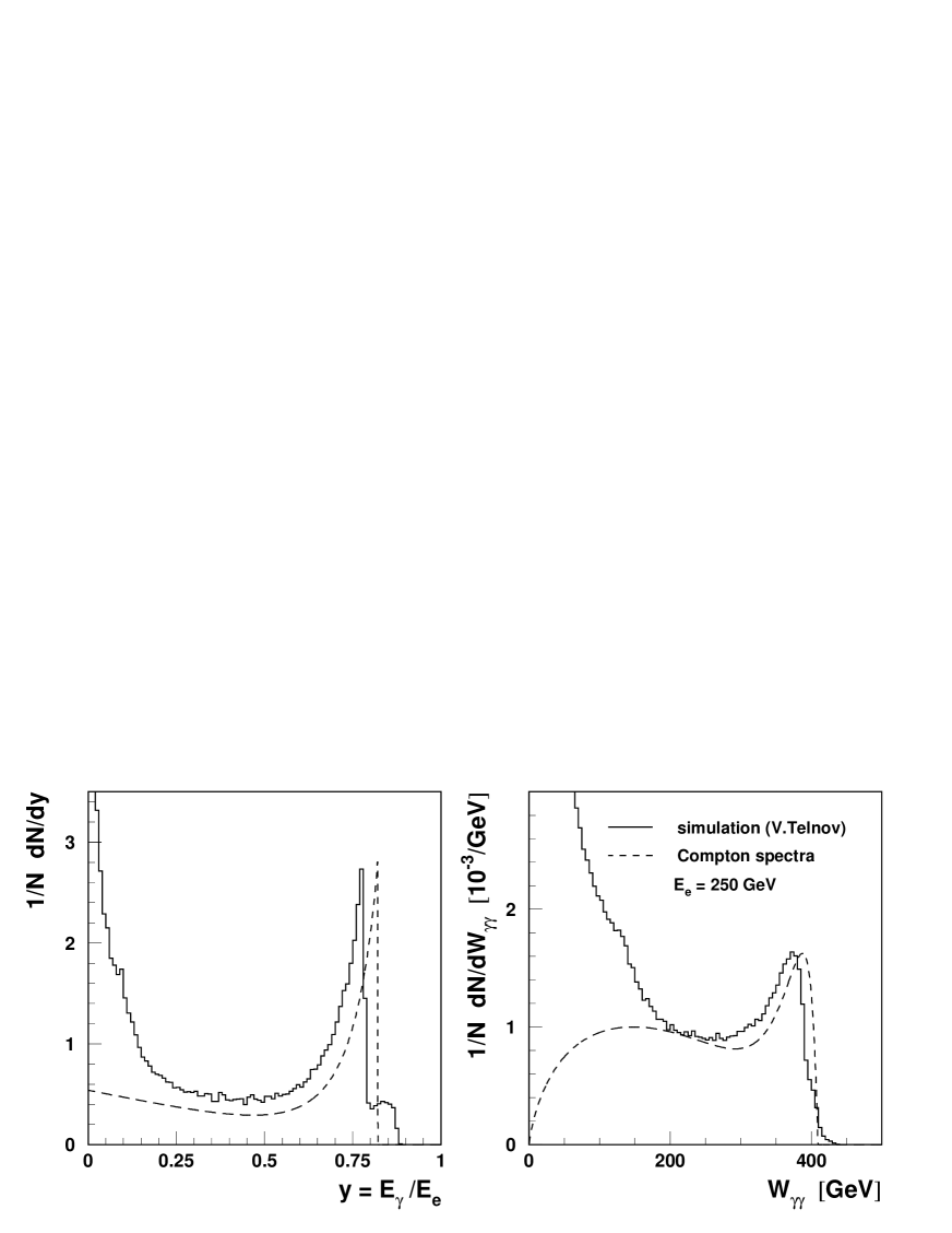
Figure 1: Energy distribution for photons (left plot) and the $\gamma\gamma$ center-of-mass energy distribution (right plot) from full simulation of luminosity spectrum by V.Telnov [7] (solid line), compared to expectations for the simple Compton scattering (dashed line). For better comparison of shape, Compton spectra is scaled to the same height of the high energy peak.

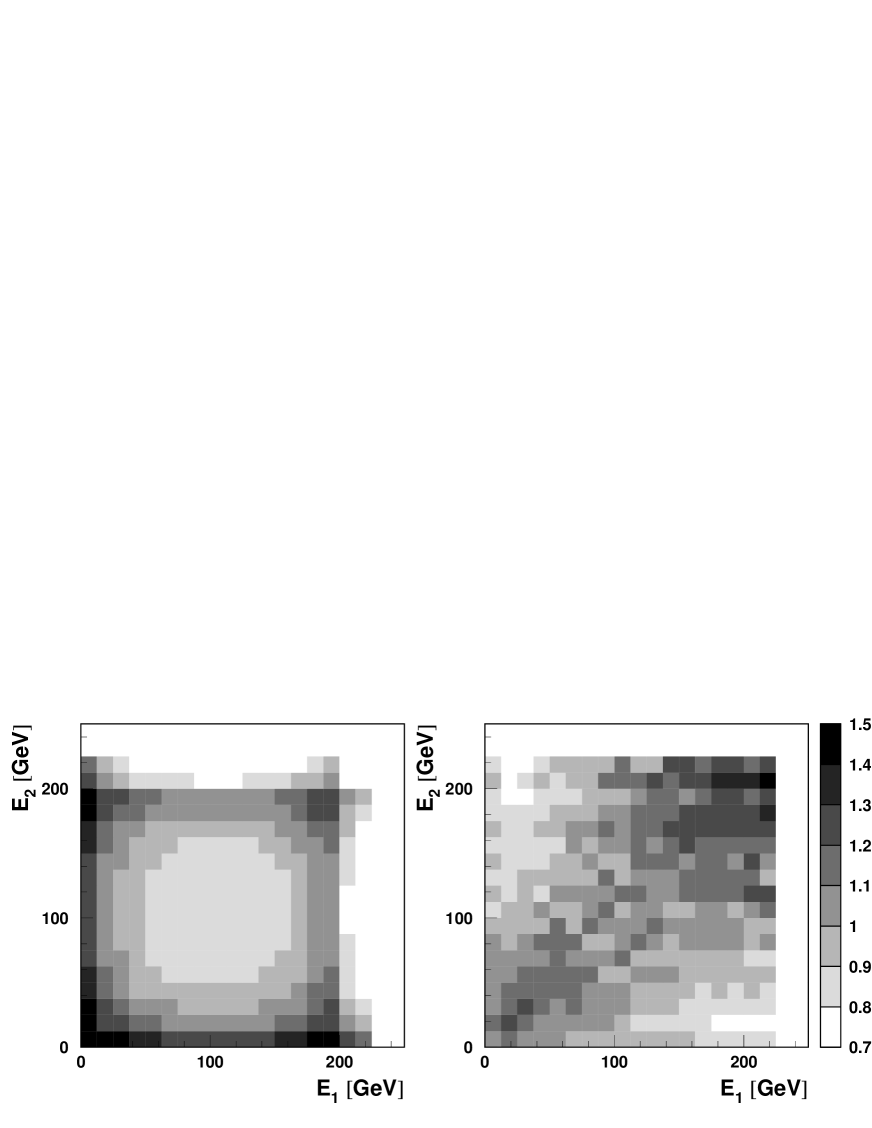
Figure 2: Two-dimensional energy distribution for two colliding photons, obtained from the full simulation by V.Telnov [7] (left plot) and the ratio of this distribution to the simple product of two one-dimensional energy spectra (right plot).

3 Model

Dedicated studies have been performed in order to understand the differences between the photon energy spectra obtained from the collider simulation by V.Telnov [7] and the spectra expected for the simple Compton scattering (14). To describe simulation results following effects are taken into account: nonlinear effects due to high density of the laser beam, correlation between photon energy and the scattering angle, electron rescattering and scattering involving two initial state laser photons.

3.1 Nonlinear effects

For very high density of the laser beam nonlinear QED effects become important. The field of the electromagnetic wave can significantly influence the motion of an electron. The effect can be described as an effective increase in the electron mass $m_{e}^{2}\rightarrow m_{e}^{2}(1+\xi^{2})$, where $\xi^{2}$ is the parameter describing the nonlinear effects, proportional to the photon density in the laser beam [12]. For the Compton scattering nonlinear effects result in an effective rescaling of the parameter $x$, describing the photon energy spectra:

$$x=\frac{4E_{0}E_{e}}{m_{e}^{2}} \longrightarrow \tilde{x}=\frac{x}{1+\xi^{2}}$$ (1)

where $E_{e}$ is the electron beam energy and $E_{0}$ the energy of the laser photon. As a result, the energy distribution for the backscattered photons is shifted towards lower energies.

3.2 Angular correlations

Electron beams collide with focused laser beams at the distance $b\sim 2$mm from the interaction point. The angular spread of scattered photons is very small (due to very high Lorenz boost), but becomes important because of the very small beam spot size. Due to the larger scattering angle, the effective vertical size of the photon beam increases at low photon energies. As a result, interactions involving low energy photons are suppressed. The effect of angular correlations can be described by the following modification of the energy spectrum [10]:

$$\frac{1}{N}\frac{dN}{dy}=f(y,\tilde{x}) = f_{C}(y,\tilde{x})\cdot{\cal N}\exp\left(-\frac{\rho^{2}}{8}\;\left(\frac{\tilde{x}}{y}-\tilde{x}-1\right)\right)\;,$$ (2)

where the parameter $\rho$ relates the vertical beam size $\sigma_{y}$ and the distance $b$ between the conversion and interaction points, $\rho\approx(m_{e}b)/(E_{e}\sigma_{y})$, ${\cal N}$ is normalization factor and $f_{C}(y,\tilde{x})$ is the Compton spectrum, as described by eq. (14) in appendix A.

3.3 Electron rescattering

With high density of the laser beam, one can ”convert” most of the electrons into the high energy photons. However, after the first scattering electrons still have large energies. Scattering of laser photons on these secondary electrons results in an additional contribution to the photon-energy spectrum. Due to the lower electron energy, secondary scattering takes place at lower $x$ value, $x^{\prime}=y^{\prime}\tilde{x}$, where $y^{\prime}$ is the energy fraction of the secondary electrons. Energy distribution for photons scattered off secondary electrons can be calculated by integrating over $y^{\prime}$:

$$\frac{1}{N^{\prime}}\frac{dN^{\prime}}{dy}=f^{\prime}(y,\tilde{x}) = {\cal N}^{\prime}\int\limits_{0}^{1}dy^{\prime}\;\;\;w_{C}(y^{\prime})\;f_{C}(1-y^{\prime},\tilde{x})\cdot f_{C}(\frac{y}{y^{\prime}},y^{\prime}\tilde{x})$$ (3)

where ${\cal N}^{\prime}$ is the normalization factor and $w_{C}(y^{\prime})$ is the weighting function which takes into account the dependence of the total Compton scattering cross section on the electron energy [3, 11]. In the high energy limit one gets

$$w_{C}(y^{\prime}) \approx \frac{\tilde{x}}{x^{\prime}}\cdot\frac{\log(x^{\prime}+1)}{\log(\tilde{x}+1)}\;.$$ (4)

Photons from scattering on secondary electrons have much “softer” energy spectrum, as compared to the Compton scattering on primary electrons.

3.4 Scattering of two laser photons

For high density of laser beam it is also possible that electron scatters on two photons instead of one. The detailed calculation of the energy distribution for photons produced in such scattering is presented in [12]. We have found that the distribution obtained from the simulation [7] can be well approximated by a simple formula for the scattering on one photon with double energy (i.e. with $\tilde{x}\rightarrow 2\tilde{x}$) corrected by an additional factor which suppresses the high energy peak:

$$\frac{1}{N_{2}}\frac{dN_{2}}{dy}=f_{2}(y,\tilde{x}) = f(y,2\tilde{x})\cdot{\cal N}_{2}\;\left(\frac{2\tilde{x}}{y}-2\tilde{x}-1\right)^{\delta}\;,$$ (5)

where $\delta$ is the parameter describing suppression of the high energy part of the spectrum and ${\cal N}_{2}$ is the normalization constant.

4 Parametrization

4.1 Main assumptions

The main aim of the presented study was to parametrize the high energy part of the luminosity spectra of the Photon Collider in a simple analytical form. It was assumed that the high energy part of the $\gamma\gamma$ luminosity spectrum can be described as a simple product:

$$\frac{1}{N}\frac{d^{2}N}{dy_{1}dy_{2}} = f_{tot}(y_{1},\tilde{x})\;f_{tot}(y_{2},\tilde{x})$$ (6)

where $f_{tot}(y,\tilde{x})$ is the energy spectrum for the photon. The spectrum can be parametrized as a sum of three components described in the previous section:

$$f_{tot}(y,\tilde{x}) = n\;f(y,\tilde{x})\;+\;n^{\prime}\;f^{\prime}(y,\tilde{x})\;+\;n_{2}\;f_{2}(y,\tilde{x})$$ (7)

where $n$, $n^{\prime}$ and $n_{2}$ are parameters describing contributions of different processes to the spectrum. All together the model has 10 free parameters which can be adjusted to describe the results of simulation by Telnov [7]. Only 4 of these parameters describe the shape of the contributing components:

• two parameters, $\xi_{0}$ and $\xi_{1}$, describing $\xi^{2}$ dependence on the electron beam energy:

  $$\xi^{2} = \xi_{0}+E_{e}\cdot\xi_{1}$$ (8)

• parameter $\rho^{2}$ describing the angular correlations

• parameter $\delta$ added in description of two-photon scattering

Remaining 6 parameters, $a_{1}\ldots a_{6}$, are needed to describe the normalization of the contributing processes:

• the dependence of the normalization of the Compton scattering contribution ($n$) on the electron beam energy is, in the considered energy range, approximately given by:

  $$n\>{\cal N}=a_{1}\cdot E_{e}\;+\;a_{2}$$ (9)

• normalization of the electron rescattering ($n^{\prime}$) and of the two photon scattering ($n_{2}$) are related to the Compton scattering contribution by the formula:

  $$n^{\prime}\>{\cal N}^{\prime} = n\>{\cal N}\cdot\left(a_{3}\cdot E_{e}\;+\;a_{4}\right)$$ (10)

  $$n_{2}\>{\cal N}_{2} = n\>{\cal N}\cdot a_{5}\left(1-\exp(-a_{6}\>\xi^{2})\right)$$ (11)

Normalization factors ${\cal N}$, ${\cal N}^{\prime}$ and ${\cal N}_{2}$ are included in the parametrization to simplify numerical calculations of the spectra.

Whereas distributions $f$, $f^{\prime}$ and $f_{2}$ are normalized to unity, normalization of $f_{tot}$ is not fixed. It is evaluated from the requirement that the high energy part of the luminosity spectrum is given by the formula (6).

4.2 Fit results

The formula (7) was compared with the photon energy spectra obtained from simulation by V.Telnov [7]. To minimize effects of energy correlations a cut on the energy of the second photon was imposed. For electron beam energy of 100, 250 and 400 GeV the cut was 40, 150 and 260 GeV, respectively. Parameters of the model were fitted to the photon spectra, for $y>0.1$, simultaneously at all energies.

Result of the fit to the photon energy distribution at $E_{e}$=250 GeV is shown in Fig. 3. Fitted contributions of different processes are also indicated. The model describes the spectra very well down to $E_{\gamma}\sim 0.1\;E_{e}$. Three processes considered in the model contribute to different parts of the spectra. By summing these contributions most of details of the distribution can be well reproduced. Very good description of the photon energy distribution is obtained for all considered energies, as shown in Fig. 4.

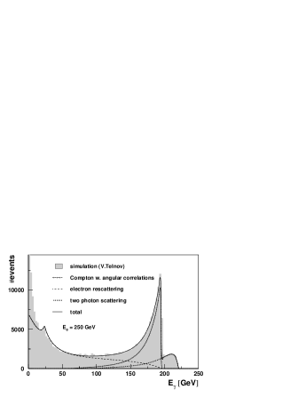
Figure 3: Comparison of the photon energy distribution obtained from full simulation of luminosity spectrum by Telnov [7], with the fitted contributions of different processes considered in the described model, as indicated in the plot.

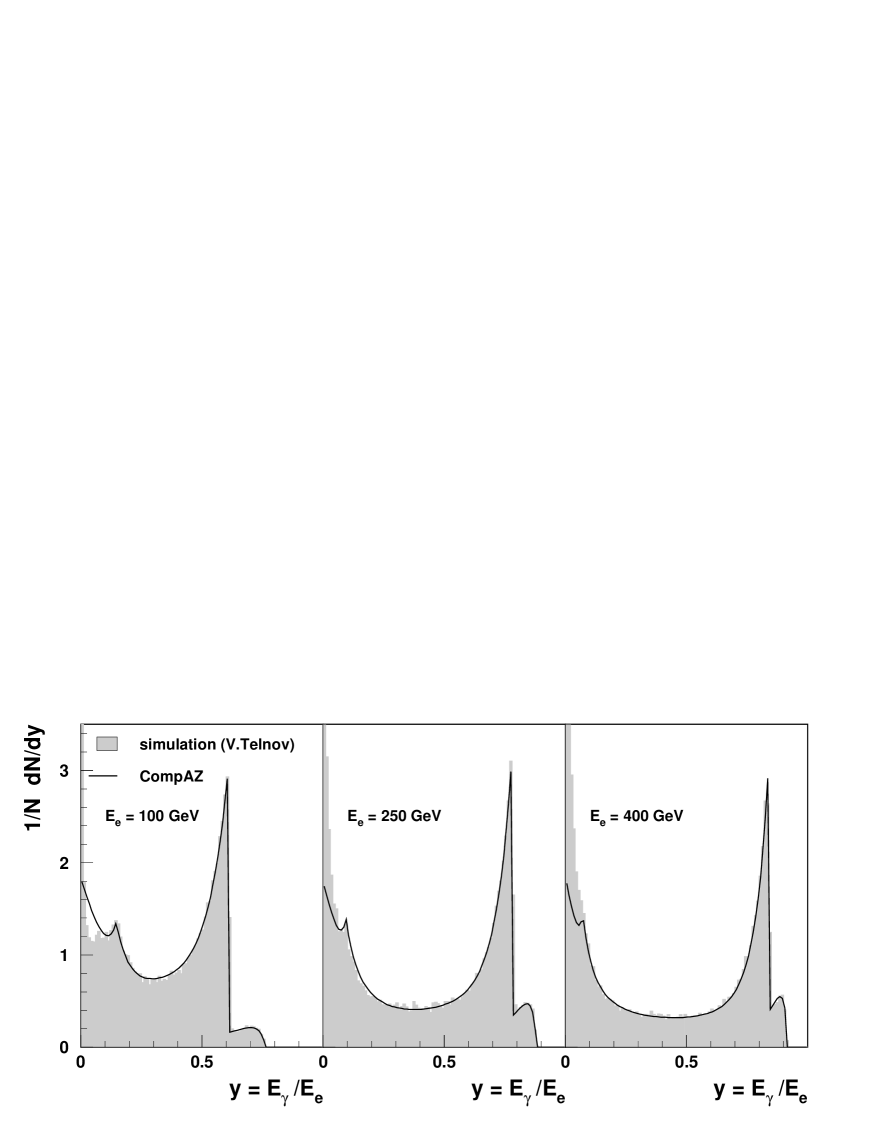
Figure 4: Comparison of the photon energy distribution from the fitted parametrization with the distribution obtained from full simulation of luminosity spectra [7], for three electron beam energies, as indicated in the plot. Imposed cut on the energy of the second photon is 40, 150 and 260 GeV respectively.

Normalization of the fitted parametrization, as well as of the contributions of different processes, are shown in Fig. 5 as a function of the electron beam energy $E_{e}$. Normalization of the parametrization changes from about 0.8 at 50 GeV to about 0.55 at 500 GeV. This means that the two photon spectrum obtained from the product of the two distributions, as given by eq. (6), describes between 65% and 30% of events expected from the spectra simulation [7]. 35% to 70% of the total $\gamma\gamma$ luminosity expected from simulation is due to events with one or two low energy photons not described by our parametrization.

Figure 5: Normalization of the CompAZ parametrization of the photon energy distribution, relative to the distribution obtained from full simulation of luminosity spectrum [7], as a function of the electron beam energy. Also shown are normalizations of separate processes considered in the model.

In Fig. 6 the comparison of the average photon polarization resulting from the fitted parametrization with the distribution obtained from the simulation of luminosity spectra is shown. To describe the photon polarization two additional assumptions were made in the model:

• scattering involving two photons results in very high photon polarization. It is taken from the Compton formula (LABEL:eq:polar) (with $\tilde{x}\rightarrow 2\tilde{x}$) for scattered photon energies above the threshold for one photon scattering, and fixed at the threshold value for lower energies;

• electrons undergoing secondary scattering are unpolarized.

Both assumptions have no strong physical motivation, however they were found to give the best description at the simulation level. It has to be stressed that the model was not fitted to the photon polarization distribution and no additional parameters were introduced to describe it. Very good agreement between the parametrization and the average photon polarization obtained from the simulation, is observed for $y>0.3$.

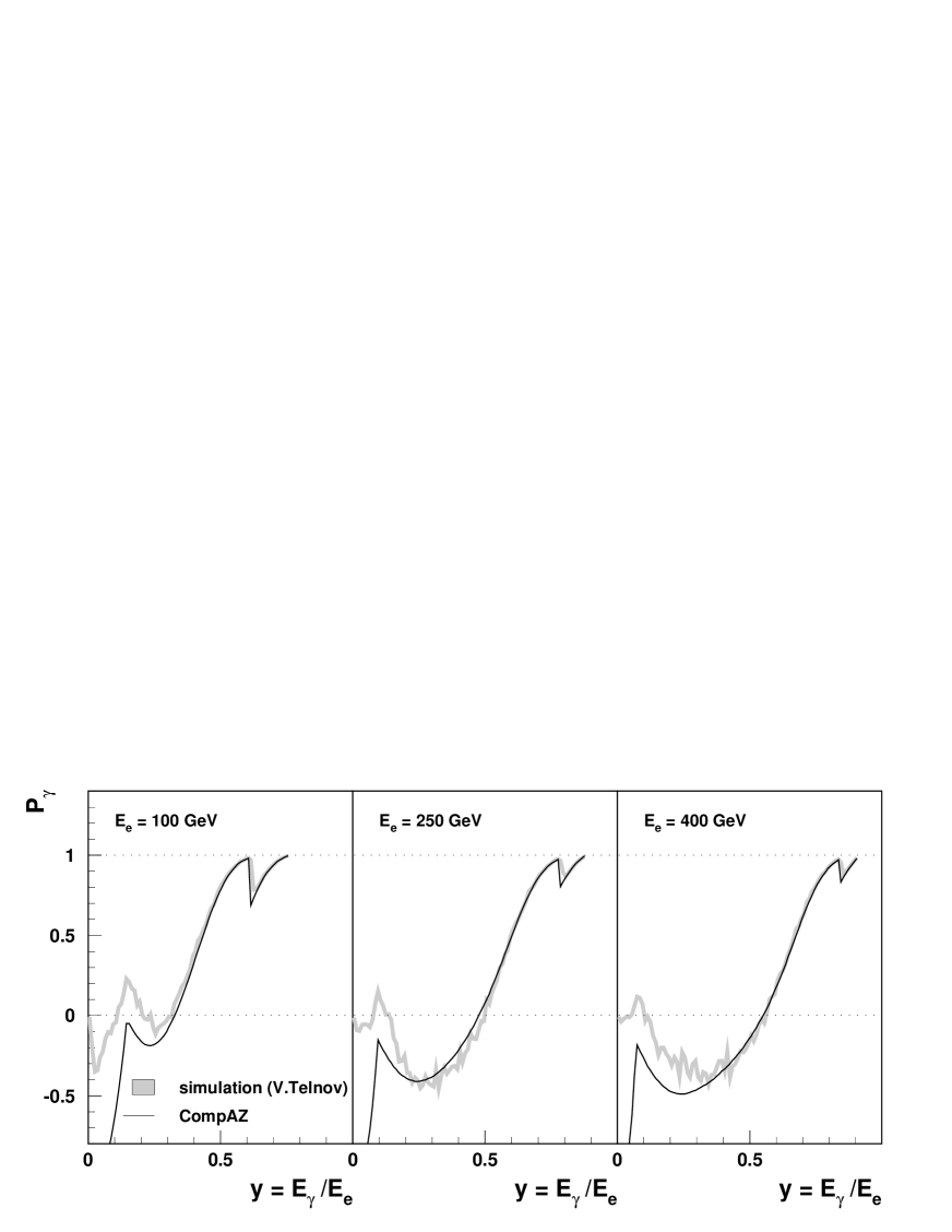
Figure 6: Comparison of the photon polarization resulting from the fitted parametrization with the distribution obtained from full simulation of luminosity spectra [7], for three electron beam energies, as indicated in the plot. Imposed cut on the energy of the second photon is 40, 150 and 260 GeV respectively.

4.3 CompAZ

The routine implementing the described spectra parametrization is called CompAZ. It can be used to calculate the photon energy spectrum for different electron beam energies and the average photon polarization for a given photon energy. Separate contributions from three considered processes (2,3,5) can also be calculated. Additional routines were prepared for convenient event generation from the parametrized spectrum. All routines can be downloaded from web [13].

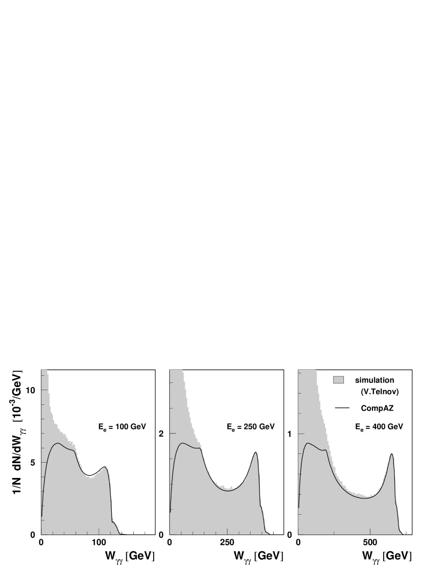
Figure 7: Comparison of the center-of-mass energy distribution obtained with the CompAZ parametrization with the distribution obtained from full simulation of luminosity spectra [7], for three electron beam energies, as indicated in the plot.

In Fig. 7 the $\gamma\gamma$ center-of-mass energy distribution obtained from CompAZ is compared with the distribution obtained from the simulation of luminosity spectra [7], for different electron beam energies. No cuts on photon energies were imposed. Proper description of the spectra is obtained for $W_{\gamma\gamma}>\sim 0.3\;W_{max}$, where $W_{max}=2\;E_{max}$ is the maximum center-of-mass energy available for two photons produced in the Compton scattering. Also the average product of the photon polarizations, related to the ratio of $\gamma\gamma$ collisions with the total angular momentum $J_{z}=0$ and $|J_{z}|=2$, is properly described for large $W_{\gamma\gamma}$ (see Fig. 8). Center-of-mass energy distribution for two colliding photons with $J_{z}=0$ is shown in Fig. 9. The parametrization describes very well the high energy part of the spectra, most relevant for many physics studies.

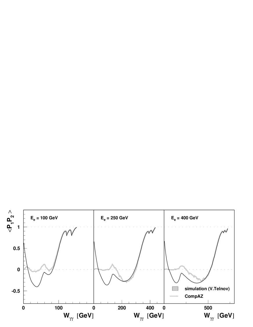
Figure 8: Comparison of the average product of photon polarizations from the CompAZ parametrization with the distribution obtained from full simulation of luminosity spectra [7], for three electron beam energies, as indicated in the plot.

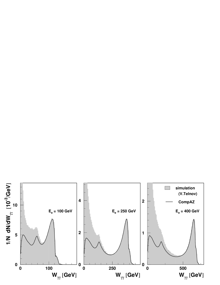
Figure 9: Center-of-mass energy distribution for two colliding photons with $J_{z}=0$. Results obtained with the CompAZ parametrization are compared with the distribution obtained from full simulation of luminosity spectra [7], for three electron beam energies, as indicated in the plot.

In the calculation of the $\gamma\gamma$ luminosity spectrum as a product of two energy distributions (6) possible energy correlations between two beams are neglected. In Fig. 10 the two-dimensional energy distribution obtained from CompAZ, and the ratio of this distribution to the two-photon spectrum obtained from the simulation by V.Telnov [7] are shown. In the high energy part of the spectrum, when both photons have high energies, $y>0.5\;y_{max}$, this ratio is close to 1. This shows that CompAZ properly describes this part of the spectrum and no additional corrections for beam energy correlations are needed. Only for $W_{\gamma\gamma}<\sim 0.3\;W_{max}$ energy correlations become important. CompAZ overestimates the number of collisions with one high energy ($y>0.5\;y_{max}$) and one low energy ($y<0.3\;y_{max}$) photon (the ratio greater than 1), and underestimates the number of collisions involving two low energy photons (the ratio smaller than 1).

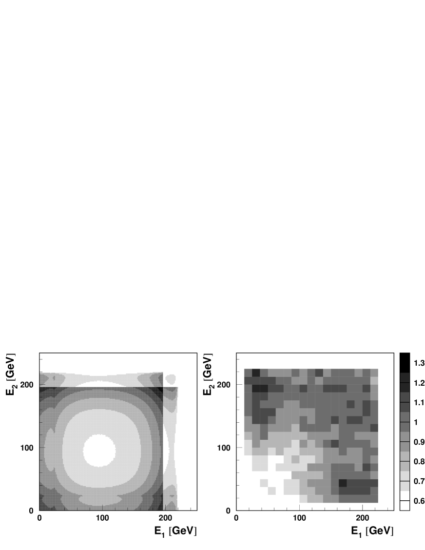
Figure 10: Two-dimensional energy distribution for two colliding photons, obtained from the CompAZ parametrization (left plot) and the ratio of this distribution to the one obtained from full simulation of luminosity spectrum [7] (right plot).

4.4 Applications

As already mentioned in the previous section, dedicated routines are available for fast simulation of $\gamma\gamma$ scattering events with CompAZ. They have been recently used in the simulation of $W^{+}W^{-}$ and $ZZ$ pair-production at the Photon Collider, for different electron beam energies [14]. Distribution of the $\gamma\gamma$ center-of-mass energy, $W_{\gamma\gamma}$ for $\gamma\gamma\rightarrow W^{+}W^{-}$ events generated with PYTHIA, for electron beam energy of 250 GeV, is shown in Fig. 11. Generated events were reweighted for photon polarizations. Sample of events generated using CompAZ is compared with the sample generated with the luminosity spectrum from simulation [6, 7]. Very good agreement is observed. The advantage of CompAZ is that it can be easily used for any beam energy, giving reasonable description of the energy and polarization.

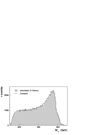
Figure 11: Distribution of the $\gamma\gamma$ center-of-mass energy for $\gamma\gamma\rightarrow W^{+}W^{-}$ events generated with PYTHIA, for electron beam energy of 250 GeV. Sample of events generated using the CompAZ parametrization is compared with the sample generated with the luminosity spectrum from full simulation. Generated events were reweighted for photon polarizations.

CompAZ parametrization can also be used for calculating expected event distributions without the time consuming event generation. Numerical integration is few orders of magnitude faster than the full simulation and can be used to extrapolate results of full simulation to other beam energies. Results from the recent study of the heavy Higgs boson production at the Photon Collider [14], for Higgs mass of 180 GeV ($h\rightarrow W^{+}W^{-}$) and 300 GeV ($h\rightarrow ZZ$) are shown in Fig. 12. Expected invariant mass distributions obtained from the full simulation, based on PYTHIA [15] and fast detector simulation program SIMDET [16], are compared with results obtained by the numerical convolution of the cross section formula for vector boson production in $\gamma\gamma$ scattering with the CompAZ photon energy spectrum and parametrization of the detector resolution. The agreement between both approaches is very good. With numerical integration based on CompAZ, it was possible to calculate the detector level effects expected from the interference between direct $W^{+}W^{-}$ production and $h\rightarrow W^{+}W^{-}$ decay. To estimate the effect with full event and detector simulation very large statistic of events would be required.

5 Summary

Luminosity spectrum obtained from the detailed beam simulation is the best tool for accurate simulation of $\gamma\gamma$ interactions. Recently the new version of CIRCE code became available [17, 18], which contains the Photon Collider luminosity spectra based on simulation by V.Telnov [6, 7]. The CIRCE program [18] gives detailed description of the luminosity spectra in the whole energy range taking properly into account all non-factorizing contributions (energy and polarization correlations). The package includes routines for convenient event generation. However, only three selected electron beam energies have been considered so far ($E_{e}$= 100, 250 and 400 GeV). Moreover, parameters of the Photon Collider assumed in the simulation are only known with accuracy up to 10–20%, as many details of the project are still not fixed. Therefore, other models resulting in the similar (or better) accuracy are also applicable for detailed studies.

We propose the model describing the photon energy spectra of the Photon Collider at TESLA in a simple analytical form, based on the formula for the Compton scattering. Parameters of the model are obtained from the comparison with the full beam simulation by V.Telnov, which includes nonlinear corrections and contributions of higher order processes. Photon energy distribution and polarization, in the high energy part of the spectra, are well reproduced in a wide range of electron beam energies. Model can be used for Monte Carlo simulation of gamma-gamma events. Parametrization is also very useful for numerical cross-section calculations.

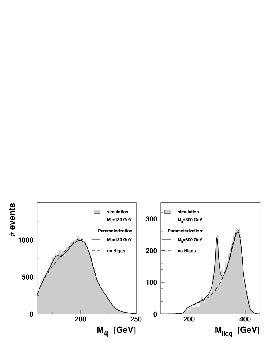
Figure 12: Distribution of the reconstructed invariant mass for $\gamma\gamma\rightarrow W^{+}W^{-}$ events with a SM Higgs-boson mass of 180 GeV and an electron-beam energy of 152.5 GeV (left plot) and for $\gamma\gamma\rightarrow ZZ$ events, with a SM Higgs-boson mass of 300 GeV and an electron-beam energy of 250 GeV (right plot). Results from the simulation based on PYTHIA and on the SIMDET detector simulation (histogram) are compared with the distribution obtained by the numerical convolution of the cross-section formula with the CompAZ photon energy spectra and parametrization of the detector resolution (solid line). The distribution expected without the Higgs contribution is also shown (dashed line).

Appendix A Energy spectrum for Compton scattering

The energy spectrum of the photons resulting from the Compton backscattering of laser light off the high energy electron beam depends on the electron beam and laser polarizations, $P_{e}$ and $P_{L}$, and on the dimension–less parameter $x$:

$$x = \frac{4E_{0}E_{e}}{m_{e}^{2}},$$ (12)

where $E_{e}$ is the electron beam energy, $E_{0}$ the energy of the laser photon and $m_{e}$ is the electron mass. The maximum energy of the scattered photon is

$$E_{max} = \frac{x}{x+1}\;E_{e}.$$ (13)

and the energy spectrum is given by [4]

$$\frac{1}{N}\frac{dN}{dy} = f_{C}(y,x)=$$ (14)

$$= \!{\cal N}_{C}\left[\frac{1}{1-y}-y+(2r-1)^{2}-\!P_{e}P_{L}\;xr(2r-1)(2-y)\right],$$

where $r=y/(x(1-y))$, $y$ is the fraction of the electron energy transfered to the photon

$$0\;\leq\;y=\frac{E_{\gamma}}{E_{e}} \leq \frac{x}{x+1}\;,$$ (15)

and ${\cal N}_{C}$ is the normalization factor given by

$$\frac{1}{{\cal N}_{C}} = \frac{1}{2}+\frac{8}{x}-\frac{1}{2(x+1)^{2}}+\left(1-\frac{4}{x}-\frac{8}{x^{2}}\right)\log(1+x)$$ (16)

$$- P_{e}P_{L}\left[2+\frac{x^{2}}{2(x+1)^{2}}-\left(1+\frac{2}{x}\right)\log(1+x)\right]\;.$$

The degree of polarization of the photons scattered with energy fraction $y$ is given by [4]

$$P_{\gamma}\! = \!\frac{\cal N_{C}}{f_{C}(y,x)}\left\{xrP_{e}\left[1+(1-y)(2r-1)^{2}\right]-(2r-1)P_{L}\left[\frac{1}{1-y}+1-y\right]\right\}.$$

The energy spectrum and polarization of the scattered photons, for $x=4.5$ and 85% polarization of the electron beam (proposed parameters of the TESLA Photon Collider for electron beam energy $E_{e}$=250 GeV), and various helicities of laser beam are shown in Fig. 13.

Figure 13: Energy distribution (left plot) and polarization (right plot) for photons from Compton back-scattering, for different laser beam polarizations $P_{L}$, as indicated in the plot. $x=4.5$ corresponds to laser wave length of 1.06 $\mu m$ and primary electron beam energy of 250 GeV. Electron beam polarization $P_{e}$=85%.

References

- [1] B. Badelek et al., Photon Collider at TESLA, TESLA Technical Design Report Part 6, Chapter 1, DESY-2001-011, ECFA-2001-209,DESY-TESLA-2001-23, DESY-TESLA-FEL-2001-05, Mar. 2001, hep-ex/0108012.
- [2] I. F. Ginzburg, G. L. Kotkin, V. G. Serbo, and V. I. Telnov. Pizma ZhETF, 34:514, 1981. JETP Lett. 34:491, 1982. Preprint INP 81-50, Novosibirsk, 1981.
- [3] I. F. Ginzburg, G. L. Kotkin, V. G. Serbo, and V. I. Telnov. Nucl. Instrum. Meth., 205:47, 1983. Preprint INP 81-102, Novosibirsk, 1981.
- [4] I. F. Ginzburg, G. L. Kotkin, S. L. Panfil, V. G. Serbo, and V. I. Telnov. Nucl. Instrum. Meth., A219:5–24, 1984.
- [5] V. I. Telnov. Nucl. Instrum. Meth., A294:72–92, 1990.
- [6] V. I. Telnov. Nucl. Instrum. Meth., A355:3, 1995.
- [7] V. I. Telnov, A Code for the simulation of luminosities and QED backgrounds at photon colliders, talk presented at Second Workshop of ECFA-DESY study, St.Malo, France, April 2002.
- [8] P. Chen, T. Ohgaki, A. Spitkovsky, T. Takahashi, and K. Yokoya. Nucl. Instrum. Meth., A397:458, 1997. physics/9704012.
- [9] V. Telnov, Nucl. Instrum. Meth., A472:43–60, 2001.
- [10] I.F. Ginzburg and G.L. Kotkin, Eur. Phys J. C13:295–300, 2000.
- [11] V.B. Berestecky, E.M. Lifshitz, L.P. Pitaevsky, Quantum electrodynamics, Nauka, Moscow, 1980.
- [12] M. Galynskii, E. Kuraev, M. Levchuk and V. I. Telnov, Nucl. Instrum. Meth., A472:267-279, 2001.
- [13] http://info.fuw.edu.pl/∼zarnecki/compaz/compaz.html
- [14] P. Nieżurawski, A.F. Żarnecki, M. Krawczyk, Journal of High Energy Physics, JHEP 0211 (2002) 034.
- [15] T. Sjostrand, P. Eden, C. Friberg, L. Lonnblad, G. Miu, S. Mrenna and E. Norrbin, Comp. Phys. Comm. 135 (2001) 238.
- [16] M. Pohl, H. J. Schreiber, DESY-99-030.
- [17] T. Ohl, Comput. Phys. Commun. 101:269, 1997.
- [18] T. Ohl, Circe Version 2.0: Beam Spectra for Simulating Linear Collider and Photon Collider Physics, WUE-ITP-2002-006.