Measurement of the Oscillation Frequency for ${B^{0}}$-${\overline{B}{}^{0}}$ Mixing using Hadronic ${B^{0}}$ Decays

Abstract

The oscillation frequency of ${B^{0}}$-${\overline{B}{}^{0}}$ mixing (${\Delta m_{d}}$) has been measured using 29.1 ${\rm{fb}^{-1}}$ of data collected with the Belle detector at KEKB. This measurement is made through the distributions of the proper decay time difference of $B$ pairs in events tagged as same- and opposite-flavor decays. In each event, one $B$ is fully reconstructed in a flavor-specific hadronic decay mode, while the flavor of the other is extracted through a likelihood calculated from the $b$-flavor information carried in its final decay products. We obtain ${\Delta m_{d}}=(0.528\pm 0.017\pm 0.011)~{}\rm{ps}^{-1}$, where the first error is statistical and the second error is systematic.

PACS: 12.15.Hh, 11.30.Er, 13.25.Hw

KEK preprint 2002-63 Belle preprint 2002-20

, , , , , , , , , , , , , , , , , , , , , , , , , , , , , , , , , , , , , , , , , , , , , , , , , , , , , , , , , , , , , , , , , , , , , , , , , , , , , , , , , , , , , , , , , , , , , , , , , , , , , , , , , , , , , , , , , , , , , , , , , , , , , , , , , , , , , , , , , , , , , , , , , , , , , , , , , , , , , , , , , , , , , , , , , , , , , , , , , , , , , , , , , , , , , , , , , , , , , , , , and

1 Introduction

In the Standard model, ${B^{0}}$-${\overline{B}{}^{0}}$ oscillation occurs through second order weak interactions where the dominant contribution has an internal loop that contains virtual $t$-quarks. As a result, the oscillation frequency ${\Delta m_{d}}$ is related to the Cabibbo-Kobayashi-Maskawa (CKM) matrix elements $V_{td}$ and $V_{tb}$ [1]. Since $|V_{tb}|$ is expected to be very close to 1, a precise measurement of ${\Delta m_{d}}$, in principle, provides a method to determine $|V_{td}|$. Although the extraction of $|V_{td}|$ from ${\Delta m_{d}}$ is currently hampered by theoretical uncertainties on hadronic matrix elements, precision measurements of ${\Delta m_{d}}$ could be important for future determinations of $|V_{td}|$. In addition, ${B^{0}}$-${\overline{B}{}^{0}}$ mixing is one of the sources of $CP$ violation in ${B^{0}}$ decays and a good knowledge of ${\Delta m_{d}}$ is important for precise measurements of these $CP$ asymmetries. Since the first observation of ${B^{0}}$-${\overline{B}{}^{0}}$ mixing [2], a number of measurements of ${\Delta m_{d}}$ have been reported [3]. Recently, asymmetric $B$-factory experiments operated at the $\Upsilon(4S)$ resonance have significantly improved the precision of ${\Delta m_{d}}$ [4].

In this letter, we present a determination of ${\Delta m_{d}}$ from the time evolution of opposite-flavor (OF; ${B^{0}}$${\overline{B}{}^{0}}$) and same-flavor (SF; ${B^{0}}$${B^{0}}$, ${\overline{B}{}^{0}}$${\overline{B}{}^{0}}$) neutral $B$ decays at the $\Upsilon(4S)$ resonance. In the absence of background and detector effects, the time-dependent probabilities of observing OF ($\mathcal{P}^{{\rm OF}}$) and SF ($\mathcal{P}^{{\rm SF}}$) states are given by

$$\mathcal{P}^{{\rm OF}}({\Delta t}) = \frac{1}{4{\tau_{{B^{0}}}}}\exp\left(-\frac{|{\Delta t}|}{{\tau_{{B^{0}}}}}\right)\left[1+\cos({\Delta m_{d}}{\Delta t})\right],$$ (1)

$$\mathcal{P}^{{\rm SF}}({\Delta t}) = \frac{1}{4{\tau_{{B^{0}}}}}\exp\left(-\frac{|{\Delta t}|}{{\tau_{{B^{0}}}}}\right)\left[1-\cos({\Delta m_{d}}{\Delta t})\right],$$ (2)

where ${\tau_{{B^{0}}}}$ is the ${B^{0}}$ lifetime, and ${\Delta t}$ is the proper time difference between the two $B$ meson decays. As the decay width difference of the two mass eigenstates of the ${B^{0}}{\overline{B}{}^{0}}$ system is expected to be very small in the Standard Model [5], we assume in this analysis that it is equal to zero.

The analysis described here is based on a 29.1 ${\rm{fb}^{-1}}$ data sample, which contains $31.3\times 10^{6}$ $B\overline{B}$ pairs, collected with the Belle detector [6] at the asymmetric-energy KEKB storage ring [7]. KEKB collides an 8.0 GeV electron beam and a 3.5 GeV positron beam with a crossing angle of 22 mrad, resulting in a center-of-mass system (cms) moving nearly along the $z$ axis (defined as anti-parallel to the positron beam) with a Lorentz boost of $(\beta\gamma)_{\Upsilon}=0.425$. Since $B$ mesons are nearly at rest in the $\Upsilon(4S)$ cms, the proper time difference ${\Delta t}$ can be approximated as ${\Delta t}\simeq\Delta z/[c(\beta\gamma)_{\Upsilon}],$ where $\Delta z$ is the distance between the decay vertices of the two $B$ mesons in $z$ (typically $200~{}\mu\mathrm{m}$). The measurement involves the reconstruction of the decay of a neutral $B$ meson in a flavor-specific hadronic mode, the determination of the $b$-flavor of the accompanying (tagging) $B$ meson, the reconstruction of the two decay vertices to determine ${\Delta t}$, and a fit of the ${\Delta t}$ distribution taking into account ${\Delta t}$ resolution and backgrounds to extract ${\Delta m_{d}}$. We use the same flavor-tagging method as for the $\sin 2\phi_{1}$ measurement [8], and the same vertex reconstruction and resolution parameters as those used in the lifetime measurements [9].

The Belle detector consists of a three-layer silicon vertex detector (SVD), a 50-layer central drift chamber (CDC), an array of aerogel Cherenkov counters (ACC), time-of-flight scintillation counters (TOF), an electromagnetic calorimeter containing CsI(Tl) crystals (ECL), and 14 layers of 4.7 cm thick iron plates interleaved with a system of resistive plate counters (KLM). All subdetectors except the KLM are located inside a 3.4 m diameter superconducting solenoid which provides a 1.5 T magnetic field. The impact parameter resolutions for charged tracks are measured to be $\sigma_{xy}^{2}=(19)^{2}+(50/(p\beta\sin^{3/2}\theta))^{2}~{}\mu\mathrm{m}^{2}$ in the plane perpendicular to the $z$ axis and $\sigma_{z}^{2}=(36)^{2}+(42/(p\beta\sin^{5/2}\theta))^{2}~{}\mu\mathrm{m}^{2}$ along the $z$ axis, where $\beta=pc/E$, $p$ and $E$ are the momentum (${\rm GeV}/c$) and energy (GeV) of the particle, and $\theta$ is the polar angle from the $z$ axis.

2 Event Selection and Reconstruction

${\overline{B}{}^{0}}$ mesons are fully reconstructed in the decay modes ${\overline{B}{}^{0}}\to{D^{+}}{\pi^{-}}$, ${D^{*+}}{\pi^{-}}$, and ${D^{*+}}{\rho^{-}}$. Charged pion and kaon candidates are required to satisfy selection criteria based on particle-identification likelihood functions derived from specific ionization (d$E$/d$x$) in the CDC, time of flight, and the response of the ACC. Photon candidates are defined as isolated ECL clusters with energy more than 30 MeV that are not matched to any charged track. We reconstruct ${\pi^{0}}$ candidates from pairs of photon candidates with invariant masses between 124 and $146~{}{\rm MeV}/c^{2}$. A mass-constrained fit is performed to improve the ${\pi^{0}}$ momentum resolution. A minimum ${\pi^{0}}$ momentum of $0.2~{}{\rm GeV}/c$ is required. We select ${\rho^{-}}$ candidates as ${\pi^{-}}{\pi^{0}}$ pairs having invariant masses within $\pm 150~{}{\rm MeV}/c^{2}$ of the nominal ${\rho^{-}}$ mass.

Neutral and charged $D$ candidates are reconstructed in the following channels: $D^{0}\to K^{-}{\pi^{+}}$, $K^{-}{\pi^{+}}{\pi^{0}}$, $K^{-}{\pi^{+}}{\pi^{+}}{\pi^{-}}$, and $D^{+}\to K^{-}{\pi^{+}}{\pi^{+}}$. Candidate ${D^{*+}}\to D^{0}{\pi^{+}}$ decays are formed by combining a $D^{0}$ candidate with a slow and positively charged track, for which no particle identification is required. We apply mode-dependent requirements on the reconstructed $D$ mass (ranging from $\pm 15$ to $\pm 58$ MeV/$c^{2}$) and the mass difference between $D^{*+}$ and $D^{0}$ (ranging from $\pm 3$ to $\pm 12$ MeV/$c^{2}$). To reduce continuum background, a mode-dependent selection is applied based on the ratio of the second to zeroth Fox-Wolfram moments [10] and the angle between the thrust axes of the reconstructed and associated $B$ mesons.

We identify $B$ decays based on requirements on the energy difference ${\Delta E}\equiv{E_{B}^{\rm cms}}-{E_{\rm beam}^{\rm cms}}$ and the beam-energy constrained mass ${M_{\rm bc}}\equiv\sqrt{({E_{\rm beam}^{\rm cms}})^{2}-({p_{B}^{\rm cms}})^{2}}$, where ${E_{B}^{\rm cms}}$ and ${p_{B}^{\rm cms}}$ are the cms energy and momentum of the fully reconstructed $B$ candidate, and ${E_{\rm beam}^{\rm cms}}$ is the cms beam energy. If more than one fully reconstructed $B$ candidate is found in the same event, the one with the best combined $\chi^{2}$ for ${\Delta E}$, ${M_{\rm bc}}$, and the invariant mass of the $D$ candidate is chosen. For each channel, a rectangular signal region is defined in the ${\Delta E}$-${M_{\rm bc}}$ plane, corresponding to $\pm 3\sigma$ windows centered on the expected means for ${\Delta E}$ and ${M_{\rm bc}}$. The ${\Delta E}$ resolution is $\sigma=10\sim 30$ MeV, depending on the decay mode and $\sigma\simeq 3~{}{\rm MeV}/c^{2}$ for ${M_{\rm bc}}$ for all modes (5.27 $<{M_{\rm bc}}<$ 5.29 GeV/$c^{2}$ is used). For the determination of background parameters, we use candidates in a background dominated (sideband) region, $-0.1$ ($-0.05$ for $D^{*+}\rho^{-}$) $<{\Delta E}<$ 0.2 GeV and 5.20 $<{M_{\rm bc}}<$ 5.29 GeV/$c^{2}$, and exclude the signal region.

Charged leptons, pions, and kaons that are not associated with the reconstructed hadronic decay are used to identify the flavor of the accompanying $B$ meson. We apply the same method that has been used for our measurement of $\sin 2\phi_{1}$ [8]. Initially, the $b$-flavor determination is performed at the track level. Several categories of well measured tracks that have a charge correlated with the $b$ flavor are selected: high momentum leptons from $b\to$ $c\ell^{-}\overline{\nu}$, lower momentum leptons from $c\to$ $s\ell^{+}\nu$, charged kaons and $\Lambda$ baryons from $b\to$ $c\to$ $s$, high momentum pions originating from decays of the type $B^{0}\to$ $D^{(*)-}X$ (where $X=\pi^{+},\rho^{+}$, $a_{1}^{+},{\rm etc.})$, and slow pions from $D^{*-}\to$ $\overline{D}{}^{0}\pi^{-}$. We use Monte Carlo (MC) simulations to determine a category-dependent variable that indicates whether a track originates from a $B^{0}$ or $\overline{B}{}^{0}$. The values of this variable range from $-1$ for a reliably identified $\overline{B}{}^{0}$ to $+1$ for a reliably identified $B^{0}$ and depend on the tagging particle’s charge, cms momentum, polar angle and particle-identification probability, as well as other kinematic and event shape quantities. The results from the separate track categories are then combined to take into account correlations in the case of multiple track-level tags. We use two parameters, $q$ and $r$, to represent the tagging information. The first, $q$, corresponds to the sign of the $b$ quark charge of the tag-side $B$ meson where $q=+1$ for $\overline{b}$ and hence $B^{0}$, and $q=-1$ for $b$ and ${\overline{B}{}^{0}}$. The parameter $r$ is an event-by-event, MC-determined flavor-tagging dilution factor that ranges from $r=0$ for no flavor discrimination to $r=1$ for unambiguous flavor assignment. It is used only to sort data into six intervals of $r$ (boundaries at 0.25, 0.5, 0.625, 0.75, 0.875), according to flavor purity. More than 99.5% of the events are assigned a non-zero value of $r$.

The decay vertices of the two $B$ mesons in each event are fitted using tracks that have at least one SVD hit in the $r$-$\phi$ plane and at least two SVD hits in the $r$-$z$ plane, under the constraint that they are consistent with the interaction point (IP) profile, smeared in the $r$-$\phi$ plane by $21~{}\mu\mathrm{m}$ to account for the transverse $B$ decay length. The IP profile is represented by a three-dimensional Gaussian, the parameters of which are determined in each run (every 60,000 events in case of the mean position) using hadronic events. The size of the IP region is typically $\sigma_{x}\simeq 100~{}\mu\mathrm{m}$, $\sigma_{y}\simeq 5~{}\mu\mathrm{m}$, and $\sigma_{z}\simeq 3$ mm, where $x$ and $y$ denote horizontal and vertical directions, respectively.

The decay point of the reconstructed ${B^{0}}$ is obtained from the vertex position and momentum vector of the reconstructed $D$ meson and a track (other than the slow ${\pi^{+}}$ candidate from ${D^{*+}}$ decay) that originates from the fully reconstructed $B$ decay. The decay vertex of the tagging $B$ meson is determined from tracks not assigned to the fully reconstructed $B$ meson; however, poorly reconstructed tracks (with a longitudinal position error in excess of $500~{}\mu\mathrm{m}$) as well as tracks likely to come from ${K^{0}_{\rm S}}$ decays (because they either form a ${K^{0}_{\rm S}}$ mass when combined with an another oppositely charged track or miss the fully reconstructed $B$ vertex by more than $500~{}\mu\mathrm{m}$ in the $r$-$\phi$ plane) are not used.

The quality of a fitted vertex is assessed only in the $z$ direction (because of the tight IP constraint in the transverse plane), using the variable $\xi\equiv(1/2n)\sum^{n}_{i}\left[(z_{\rm after}^{i}-z_{\rm before}^{i})/\varepsilon_{\rm before}^{i}\right]^{2}$, where $n$ is the number of tracks used in the fit, $z_{\rm before}^{i}$ and $z_{\rm after}^{i}$ are the $z$ positions of each track (at the closest approach to the origin) before and after the vertex fit, respectively, and $\varepsilon_{\rm before}^{i}$ is the error of $z_{\rm before}^{i}$. A MC study shows that $\xi$ does not depend on the $B$ decay length. We require $\xi<100$ to eliminate poorly reconstructed vertices. About 3% of the fully reconstructed vertices and 1% of the tagging $B$ decay vertices are rejected. The proper-time difference between the fully reconstructed and the associated $B$ decays, ${\Delta t}\equiv t_{\rm rec}-t_{\rm tag}$, is calculated as ${\Delta t}=({z_{\rm{rec}}}-{z_{\rm{tag}}})/[c(\beta\gamma)_{\Upsilon}]$, where ${z_{\rm{rec}}}$ and ${z_{\rm{tag}}}$ are the $z$ coordinates of the fully-reconstructed and associated $B$ decay vertices, respectively. We reject a small fraction ($\sim$0.2%) of the events by requiring $|{\Delta t}|<70$ ps ($\sim$45${\tau_{{B^{0}}}}$).

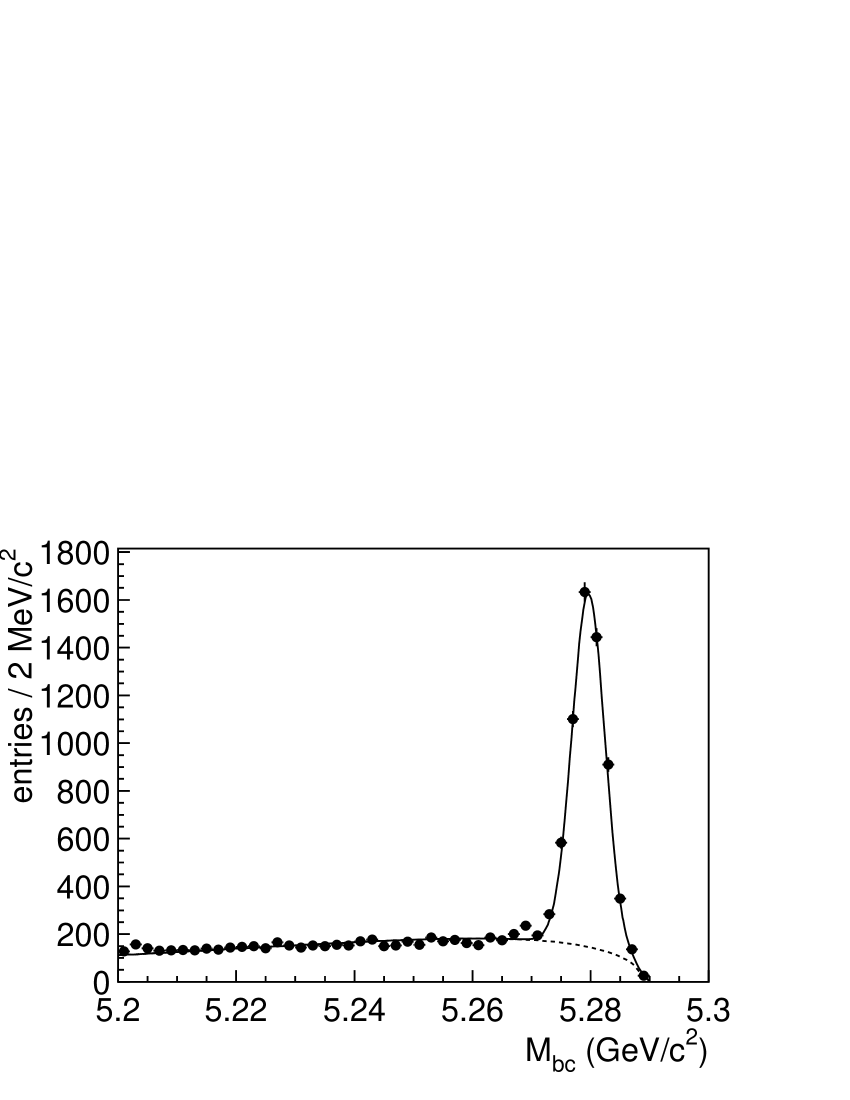
Figure 1: Beam-energy constrained mass distribution of the fully reconstructed $B^{0}$ candidates. The dashed curve shows the background contributions and the solid curve shows the sum of signal and background.

Figure 1 shows the ${M_{\rm bc}}$ distribution for all the candidates found in the ${\Delta E}$ signal region after flavor tagging and vertex reconstruction. We find 2269 $D^{+}\pi^{-}$, 2490 $D^{*+}\pi^{-}$, and 1901 $D^{*+}\rho^{-}$ candidates in the signal region with average purities of 86%, 81%, and 70%, respectively. The flavor-tagging intervals $l=1,2,\cdots 6$ contain 2675, 981, 597, 702, 779, and 926 candidates, respectively.

3 Extraction of $\Delta m_{\bf\it d}$

An unbinned maximum likelihood fit is performed to extract ${\Delta m_{d}}$, based on a likelihood function defined as $L({\Delta m_{d}},w_{1},w_{2},\cdots,w_{6})=\prod_{i}\tilde{P}^{{\rm OF}}({\Delta t}_{i})\times\prod_{j}\tilde{P}^{{\rm SF}}({\Delta t}_{j})$, where the index $i$ ($j$) runs over all selected OF(SF) events in the signal region. The probability density function (PDF), $\tilde{P}^{{\rm OF}({\rm SF})}$, is expressed as

$$\tilde{P}^{{\rm OF}({\rm SF})}({\Delta t}) = f_{\rm sig}[(1-f_{\rm ol})P_{\rm sig}^{{\rm OF}({\rm SF})}({\Delta t};{\Delta m_{d}},w_{l})+f_{\rm ol}f_{\rm sig}^{{\rm OF}({\rm SF})}P_{\rm ol}({\Delta t})]$$ (3)

$$+ (1-f_{\rm sig})[(1-f_{\rm ol})P_{\rm bkg}^{{\rm OF}({\rm SF})}({\Delta t})+f_{\rm ol}f_{\rm bkg}^{{\rm OF}({\rm SF})}P_{\rm ol}({\Delta t})],$$

where $f_{\rm sig}$ is a signal purity, described below, and $w_{l}$ is the wrong tag fraction of the flavor-tagging interval $l$ containing event $i$ or $j$. The signal PDF ($P^{{\rm OF}({\rm SF})}_{\rm sig}$) is the convolution of the true PDF with the resolution function ($R_{\rm sig}$). The background PDF (${P^{{\rm OF}}_{\rm bkg}}$^(SF)) is expressed in a similar way:

$$P_{k}^{{\rm OF}({\rm SF})}({\Delta t})=\int_{-\infty}^{+\infty}\mathrm{d}({{\Delta t}^{\prime}})\mathcal{P}_{k}^{{\rm OF}({\rm SF})}({{\Delta t}^{\prime}})R_{k}({\Delta t}-{{\Delta t}^{\prime}}),$$ (4)

where $k$ = sig, bkg. A small number of signal and background events have large ${\Delta t}$ values. We account for the contribution from these “outliers” by adding a Gaussian component ${P_{\rm ol}}({\Delta t})$ with a width and contribution fraction determined from our $B$ lifetime analysis [9]. The width of the outlier Gaussian is $\sigma_{\rm ol}$ = 36 ps, and the fraction, $f_{\rm ol}$, is 0.06% if both vertices are reconstructed from two or more charged tracks and 3.1% if at least one vertex is reconstructed from a single track constrained with the IP profile. We assume $f_{\rm ol}$ to be the same for signal and background as well as for the OF and SF sub-samples. $f_{k}^{{\rm OF}({\rm SF})}$ is the fraction of OF(SF) events for $k$ (= sig, bkg) and given by $N_{k}^{{\rm OF}({\rm SF})}/(N_{k}^{{\rm OF}}+N_{k}^{{\rm SF}})$, where $N_{k}^{{\rm OF}({\rm SF})}$ is the number of OF(SF) events in the signal region for $k$ from the result of the ${\Delta E}{}$-${M_{\rm bc}}{}$ distribution fit described below.

The signal purity ($f_{\rm sig}$) is determined on an event-by-event basis as a function of ${\Delta E}$ and ${M_{\rm bc}}$. The two-dimensional distribution of these variables including the sideband region is fitted with the sum of a Gaussian function ${F_{\rm sig}}({\Delta E},{M_{\rm bc}})$ to represent the signal, and a background function ${F_{\rm bkg}}({\Delta E},{M_{\rm bc}})$, represented as an ARGUS background function [11] in ${M_{\rm bc}}$ and a first-order polynomial in ${\Delta E}$. The fraction of signal is taken to be $f_{\rm sig}({\Delta E},{M_{\rm bc}})={F_{\rm sig}}/[{F_{\rm sig}}+{F_{\rm bkg}}]$. The fits are done separately for the three $B$ decay modes, and the dependence of the signal fraction on the flavor-tag interval $l$ is included in the overall normalization of $f_{\rm sig}$.

In order to account for wrong tagging, the true signal PDF ($\mathcal{P}_{\rm sig}^{{\rm OF}({\rm SF})}$) is given by replacing $\cos({\Delta m_{d}}{\Delta t})$ with $(1-2w_{l})\cos({\Delta m_{d}}{\Delta t})$ in Eq. 1 (Eq. 2). The resolution function of the signal is constructed by convolving four different contributions: the detector resolutions on ${z_{\rm{rec}}}$ and ${z_{\rm{tag}}}$, the smearing of ${z_{\rm{tag}}}$ due to the inclusion of tracks which do not originate from the associated $B$ vertex, mostly due to charm and $K_{\rm S}$ decays, and the kinematic approximation that the $B$ mesons are at rest in the cms. The resolution is determined on an event-by-event basis, using the estimated uncertainties on the vertex $z$ positions determined from the vertex fit. The parameterization of the resolution depends on whether the vertices are reconstructed with multiple tracks or a single track. A detailed description of the resolution parameterization can be found in Ref. [9]. We use the same parameters for $R_{\rm sig}({\Delta t})$ obtained there for this analysis. The average ${\Delta t}$ resolution for the signal is $\sim$1.56 ps (rms).

The background PDF is modeled as a sum of exponential and prompt components,

$$\mathcal{P}_{\rm bkg}^{{\rm OF}({\rm SF})}({\Delta t}) = f^{{\rm OF}({\rm SF})}_{\rm bkg}\left[f^{\delta}_{\rm bkg}\delta({\Delta t}-\mu_{\delta}^{\rm bkg})+\frac{(1-f^{\delta}_{\rm bkg})}{2{\tau_{\rm bkg}}}e^{-|{\Delta t}-\mu_{\tau}^{\rm bkg}|/{{\tau_{\rm bkg}}}}\right],$$ (5)

convolved with $R_{\rm bkg}({\Delta t})$, which is parameterized as a sum of two Gaussians. Different parameter values are used for $R_{\rm bkg}({\Delta t})$ depending on whether or not both vertices are reconstructed with multiple tracks. The parameters for the background PDF are determined using the ${\Delta E}$-${M_{\rm bc}}$ sideband region for each decay mode. A MC study shows that the fraction of prompt component in the signal region is smaller (by $\sim$10–50% depending on the decay mode) than that in the sideband region. We correct the estimates of $f_{\rm bkg}^{\delta}$ for this effect.

In the final fit, we fix ${\tau_{{B^{0}}}}$ to the world average value [13] and determine ${\Delta m_{d}}$ and $w_{l}$ ($l$=1,6). The fit result is listed in Table 1. Separate fits to the ${D^{+}}{\pi^{-}}$, ${D^{*+}}{\pi^{-}}$, and ${D^{*+}}{\rho^{-}}$ decay modes give consistent ${\Delta m_{d}}$ values: 0.536 $\pm$ 0.027 ps^-1, 0.543 $\pm$ 0.027 ps^-1, and 0.497 $\pm$ 0.032 ps^-1, respectively. Figure 2 shows the ${\Delta t}$ distributions for OF and SF events with the fitted curves superimposed; Fig. 3 shows the asymmetry between OF and SF events, $(N_{{\rm OF}}-N_{{\rm SF}})/(N_{{\rm OF}}+N_{{\rm SF}})$, as a function of $|{\Delta t}|$.

The systematic errors are summarized in Table 2. The dominant sources are the uncertainties in the resolution functions. The fit is repeated after varying the parameters determined from the data (MC) by $\pm 1\sigma$ ($\pm 2\sigma$). The systematic error due to the modeling of the resolution function is estimated by comparing the results with different parameterizations. The systematic error due to the IP constraint is estimated by varying ($\pm 10~{}\mu\mathrm{m}$) the smearing used to account for the transverse $B$ decay length. The IP profile is determined using two different methods and we find no difference between the results. Possible systematic effects due to the track quality selection of the associated $B$ decay vertices are studied by varying each criterion by 10%. The fit quality criterion for reconstructed vertices is varied from $\xi<50$ to $\xi<200$. We check the systematic uncertainty due to outliers by varying the ${\Delta t}$ range to $\pm 40$ ps and $\pm 100$ ps, and find a negligibly small effect. ${\Delta E}$-${M_{\rm bc}}$ signal regions are varied by $\pm 10$ MeV for ${\Delta E}$ and $\pm 3~{}{\rm MeV}/c^{2}$ for ${M_{\rm bc}}$. The parameters determining $f_{\rm sig}$ are varied by $\pm 1\sigma$ to estimate the associated systematic error. We study background components with a MC sample that includes both $B\overline{B}$ and continuum events. We find no significant peaking background in the signal region above the fitted background curve and conclude that the effect of peaking background is negligibly small. The systematic error due to the background shape is estimated by varying its parameters by their errors. In the nominal fit, we do not include any oscillation component in the background; such a component may arise from the ${B^{0}}$ originated background. We repeat the fit with a background PDF including a mixing term, where background parameters are taken from the sideband data. The dependence on the ${B^{0}}$ lifetime is measured by varying the lifetime by $\pm 1\sigma$ from the world average value. The possible bias in the fitting procedure and the effect of SVD alignment error are studied with MC samples; we find no bias. The MC statistical error is associated as a systematic error for these sources.

4 Conclusion

We have presented a new measurement of ${\Delta m_{d}}$ using $29.1~{}{\rm{fb}^{-1}}$ of data collected with the Belle detector at the $\Upsilon(4S)$ energy. An unbinned maximum likelihood fit to the distribution of the proper-time difference of a flavor-tagged sample with one of the neutral $B$ mesons fully reconstructed in hadronic decays yields

$${\Delta m_{d}}=0.528\pm 0.017{\rm(stat)}\pm 0.011{\rm(syst)}{\rm~{}~{}ps}^{-1}.$$

This result has similar precision and is consistent with other recent measurements at asymmetric $B$-factories at the $\Upsilon(4S)$ [4], which are achieving higher precision than those at higher energies. Additionally, this measurement confirms the validity of the $\sin 2\phi_{1}$ measurement performed on the same data sample [8], since it is based on the same flavor-tagging method, and vertexing and fitting procedures.

Table 1: Summary of fit result.

Fit parameter	Fit value	Fit parameter	Fit value
${\Delta m_{d}}$	$0.528\pm 0.017$ ps-1
$w_{1}$	0.478 $\pm$ 0.017	$w_{2}$	0.313 $\pm$ 0.027
$w_{3}$	0.212 $\pm$ 0.030	$w_{4}$	0.187 $\pm$ 0.027
$w_{5}$	0.088 $\pm$ 0.022	$w_{6}$	0.016 $\pm$ 0.013

Table 2: Summary of systematic errors.

Source	Error (ps-1)
Resolution parameters	$0.008$
Resolution parameterizations	$0.003$
IP constraint	$0.001$
Track selection	$0.002$
Vertex selection	$0.003$
${\Delta E}$-${M_{\rm bc}}$ signal box	$0.001$
Signal fraction	$0.001$
Background shape	$0.002$
Mixing in the background	$0.002$
${B^{0}}$ lifetime	$0.002$
Fit bias	$0.005$
Total	$0.011$

Figure 2: Distributions of ${\Delta t}$ for (a) SF and (b) OF events with the fitted curves superimposed. The dashed, dotted, and solid curves show the background, outliers, and the sum of backgrounds and signal, respectively.

Figure 3: Time dependence of the asymmetry between OF and SF events. The curve shows the result of the ${\Delta m_{d}}$ fit.

References

- [1] M. Kobayashi and T. Maskawa, Prog. of Theor. Phys. 49 (1973) 652; N. Cabibbo, Phys. Rev. Lett. 10 (1963) 531.
- [2] H. Albrecht et al., ARGUS Collaboration, Phys. Lett. B192 (1987) 245.
-
[3]
B Oscillations Working Group, see
http://www.cern.ch/LEPBOSC/ and references therein. - [4] K. Abe et al., Belle Collaboration, Phys. Rev. Lett. 86 (2001) 3228; K. Hara et al., Belle Collaboration, to be submitted to Phys. Rev. Lett.; B. Aubert et al., BaBar Collaboration, Phys. Rev. Lett. 88 (2002) 221802; B. Aubert et al., BaBar Collaboration, Phys. Rev. Lett. 88 (2002) 221803.
- [5] A.J. Buras, W. Slominski, and H. Steger, Nucl. Phys. B245 (1984) 369.
- [6] A. Abashian et al., Belle Collaboration, Nucl. Instr. and Meth. A479 (2002) 117.
- [7] E. Kikutani ed., KEK Preprint 2001-157 (2001), to appear in Nucl. Instr. and Meth. A.
- [8] K. Abe et al., Belle Collaboration, Phys. Rev. Lett. 87 (2001) 091802; hep-ex/0202027, to appear in Phys. Rev. D.
- [9] K. Abe et al., Belle Collaboration, Phys. Rev. Lett. 88 (2002) 171801.
- [10] G.C. Fox and S. Wolfram, Phys. Rev. Lett. 41 (1978) 1581.
- [11] ARGUS Collaboration, H. Albrecht et al., Phys. Lett. B241 (1990) 278.
- [12] I. Dunietz, Phys. Lett. B427 (1998) 179.
- [13] D. E. Groom et al. (Particle Data Group), Eur. Phys. J. C15 (2000) 1.