EUROPEAN ORGANIZATION FOR NUCLEAR RESEARCH

CERN-EP-2002-032

14. May 2002

Decay-mode independent searches for new
scalar bosons with the OPAL detector at LEP

The OPAL Collaboration

Abstract

This paper describes topological searches for neutral scalar bosons $\mathrm{S}^{0}$ produced in association with a $\mathrm{Z}^{0}$ boson via the Bjorken process $\mathrm{e}^{+}\mathrm{e}^{-}\to\mathrm{S}^{0}{}\mathrm{Z}^{0}$ at centre-of-mass energies of 91 GeV and 183–209 GeV. These searches are based on studies of the recoil mass spectrum of $\mathrm{Z}^{0}\to\mathrm{e}^{+}\mathrm{e}^{-}$ and $\mu^{+}\mu^{-}$ events and on a search for $\mathrm{S}^{0}\mathrm{Z}^{0}$ with $\mathrm{Z}^{0}\to\nu\bar{\nu}$ and $\mathrm{S}^{0}\to\mathrm{e}^{+}\mathrm{e}^{-}$ or photons. They cover the decays of the $\mathrm{S}^{0}$ into an arbitrary combination of hadrons, leptons, photons and invisible particles as well as the possibility that it might be stable.

No indication for a signal is found in the data and upper limits on the cross section of the Bjorken process are calculated. Cross-section limits are given in terms of a scale factor $k$ with respect to the Standard Model cross section for the Higgs-strahlung process $\mathrm{e}^{+}\mathrm{e}^{-}\to\mathrm{H}^{0}_{\mathrm{SM}}\mathrm{Z}^{0}$.

These results can be interpreted in general scenarios independently of the decay modes of the $\mathrm{S}^{0}$. The examples considered here are the production of a single new scalar particle with a decay width smaller than the detector mass resolution, and for the first time, two scenarios with continuous mass distributions, due to a single very broad state or several states close in mass.

(Submitted to Eur. Phys. J.)

The OPAL Collaboration

G. Abbiendi², C. Ainsley⁵, P.F. Åkesson³, G. Alexander²², J. Allison¹⁶, P. Amaral⁹, G. Anagnostou¹, K.J. Anderson⁹, S. Arcelli², S. Asai²³, D. Axen²⁷, G. Azuelos^18,a, I. Bailey²⁶, E. Barberio⁸, R.J. Barlow¹⁶, R.J. Batley⁵, P. Bechtle²⁵, T. Behnke²⁵, K.W. Bell²⁰, P.J. Bell¹, G. Bella²², A. Bellerive⁶, G. Benelli⁴, S. Bethke³², O. Biebel³², I.J. Bloodworth¹, O. Boeriu¹⁰, P. Bock¹¹, D. Bonacorsi², M. Boutemeur³¹, S. Braibant⁸, L. Brigliadori², R.M. Brown²⁰, K. Buesser²⁵, H.J. Burckhart⁸, J. Cammin³, S. Campana⁴, R.K. Carnegie⁶, B. Caron²⁸, A.A. Carter¹³, J.R. Carter⁵, C.Y. Chang¹⁷, D.G. Charlton^1,b, I. Cohen²², A. Csilling^8,g, M. Cuffiani², S. Dado²¹, G.M. Dallavalle², S. Dallison¹⁶, A. De Roeck⁸, E.A. De Wolf⁸, K. Desch²⁵, M. Donkers⁶, J. Dubbert³¹, E. Duchovni²⁴, G. Duckeck³¹, I.P. Duerdoth¹⁶, E. Elfgren¹⁸, E. Etzion²², F. Fabbri², L. Feld¹⁰, P. Ferrari¹², F. Fiedler³¹, I. Fleck¹⁰, M. Ford⁵, A. Frey⁸, A. Fürtjes⁸, P. Gagnon¹², J.W. Gary⁴, G. Gaycken²⁵, C. Geich-Gimbel³, G. Giacomelli², P. Giacomelli², M. Giunta⁴, J. Goldberg²¹, E. Gross²⁴, J. Grunhaus²², M. Gruwé⁸, P.O. Günther³, A. Gupta⁹, C. Hajdu²⁹, M. Hamann²⁵, G.G. Hanson⁴, K. Harder²⁵, A. Harel²¹, M. Harin-Dirac⁴, M. Hauschild⁸, J. Hauschildt²⁵, C.M. Hawkes¹, R. Hawkings⁸, R.J. Hemingway⁶, C. Hensel²⁵, G. Herten¹⁰, R.D. Heuer²⁵, J.C. Hill⁵, K. Hoffman⁹, R.J. Homer¹, D. Horváth^29,c, R. Howard²⁷, P. Hüntemeyer²⁵, P. Igo-Kemenes¹¹, K. Ishii²³, H. Jeremie¹⁸, P. Jovanovic¹, T.R. Junk⁶, N. Kanaya²⁶, J. Kanzaki²³, G. Karapetian¹⁸, D. Karlen⁶, V. Kartvelishvili¹⁶, K. Kawagoe²³, T. Kawamoto²³, R.K. Keeler²⁶, R.G. Kellogg¹⁷, B.W. Kennedy²⁰, D.H. Kim¹⁹, K. Klein¹¹, A. Klier²⁴, M. Klute³, S. Kluth³², T. Kobayashi²³, M. Kobel³, T.P. Kokott³, S. Komamiya²³, L. Kormos²⁶, R.V. Kowalewski²⁶, T. Krämer²⁵, T. Kress⁴, P. Krieger^6,l, J. von Krogh¹¹, D. Krop¹², M. Kupper²⁴, P. Kyberd¹³, G.D. Lafferty¹⁶, H. Landsman²¹, D. Lanske¹⁴, J.G. Layter⁴, A. Leins³¹, D. Lellouch²⁴, J. Letts¹², L. Levinson²⁴, J. Lillich¹⁰, S.L. Lloyd¹³, F.K. Loebinger¹⁶, J. Lu²⁷, J. Ludwig¹⁰, A. Macpherson^28,i, W. Mader³, S. Marcellini², T.E. Marchant¹⁶, A.J. Martin¹³, J.P. Martin¹⁸, G. Masetti², T. Mashimo²³, P. Mättig^m, W.J. McDonald²⁸, J. McKenna²⁷, T.J. McMahon¹, R.A. McPherson²⁶, F. Meijers⁸, P. Mendez-Lorenzo³¹, W. Menges²⁵, F.S. Merritt⁹, H. Mes^6,a, A. Michelini², S. Mihara²³, G. Mikenberg²⁴, D.J. Miller¹⁵, S. Moed²¹, W. Mohr¹⁰, T. Mori²³, A. Mutter¹⁰, K. Nagai¹³, I. Nakamura²³, H.A. Neal³³, R. Nisius⁸, S.W. O’Neale¹, A. Oh⁸, A. Okpara¹¹, M.J. Oreglia⁹, S. Orito²³, C. Pahl³², G. Pásztor^8,g, J.R. Pater¹⁶, G.N. Patrick²⁰, J.E. Pilcher⁹, J. Pinfold²⁸, D.E. Plane⁸, B. Poli², J. Polok⁸, O. Pooth¹⁴, M. Przybycień^8,j, A. Quadt³, K. Rabbertz⁸, C. Rembser⁸, P. Renkel²⁴, H. Rick⁴, J.M. Roney²⁶, S. Rosati³, Y. Rozen²¹, K. Runge¹⁰, D.R. Rust¹², K. Sachs⁶, T. Saeki²³, O. Sahr³¹, E.K.G. Sarkisyan^8,j, A.D. Schaile³¹, O. Schaile³¹, P. Scharff-Hansen⁸, J. Schieck³², T. Schoerner-Sadenius⁸, M. Schröder⁸, M. Schumacher³, C. Schwick⁸, W.G. Scott²⁰, R. Seuster^14,f, T.G. Shears^8,h, B.C. Shen⁴, C.H. Shepherd-Themistocleous⁵, P. Sherwood¹⁵, G. Siroli², A. Skuja¹⁷, A.M. Smith⁸, R. Sobie²⁶, S. Söldner-Rembold^10,d, S. Spagnolo²⁰, F. Spano⁹, A. Stahl³, K. Stephens¹⁶, D. Strom¹⁹, R. Ströhmer³¹, S. Tarem²¹, M. Tasevsky⁸, R.J. Taylor¹⁵, R. Teuscher⁹, M.A. Thomson⁵, E. Torrence¹⁹, D. Toya²³, P. Tran⁴, T. Trefzger³¹, A. Tricoli², I. Trigger⁸, Z. Trócsányi^30,e, E. Tsur²², M.F. Turner-Watson¹, I. Ueda²³, B. Ujvári^30,e, B. Vachon²⁶, C.F. Vollmer³¹, P. Vannerem¹⁰, M. Verzocchi¹⁷, H. Voss⁸, J. Vossebeld⁸, D. Waller⁶, C.P. Ward⁵, D.R. Ward⁵, P.M. Watkins¹, A.T. Watson¹, N.K. Watson¹, P.S. Wells⁸, T. Wengler⁸, N. Wermes³, D. Wetterling¹¹ G.W. Wilson^16,k, J.A. Wilson¹, G. Wolf²⁴, T.R. Wyatt¹⁶, S. Yamashita²³, V. Zacek¹⁸, D. Zer-Zion⁴, L. Zivkovic²⁴

¹School of Physics and Astronomy, University of Birmingham, Birmingham B15 2TT, UK
²Dipartimento di Fisica dell’ Università di Bologna and INFN, I-40126 Bologna, Italy
³Physikalisches Institut, Universität Bonn, D-53115 Bonn, Germany
⁴Department of Physics, University of California, Riverside CA 92521, USA
⁵Cavendish Laboratory, Cambridge CB3 0HE, UK
⁶Ottawa-Carleton Institute for Physics, Department of Physics, Carleton University, Ottawa, Ontario K1S 5B6, Canada
⁸CERN, European Organisation for Nuclear Research, CH-1211 Geneva 23, Switzerland
⁹Enrico Fermi Institute and Department of Physics, University of Chicago, Chicago IL 60637, USA
¹⁰Fakultät für Physik, Albert-Ludwigs-Universität Freiburg, D-79104 Freiburg, Germany
¹¹Physikalisches Institut, Universität Heidelberg, D-69120 Heidelberg, Germany
¹²Indiana University, Department of Physics, Swain Hall West 117, Bloomington IN 47405, USA
¹³Queen Mary and Westfield College, University of London, London E1 4NS, UK
¹⁴Technische Hochschule Aachen, III Physikalisches Institut, Sommerfeldstrasse 26-28, D-52056 Aachen, Germany
¹⁵University College London, London WC1E 6BT, UK
¹⁶Department of Physics, Schuster Laboratory, The University, Manchester M13 9PL, UK
¹⁷Department of Physics, University of Maryland, College Park, MD 20742, USA
¹⁸Laboratoire de Physique Nucléaire, Université de Montréal, Montréal, Quebec H3C 3J7, Canada
¹⁹University of Oregon, Department of Physics, Eugene OR 97403, USA
²⁰CLRC Rutherford Appleton Laboratory, Chilton, Didcot, Oxfordshire OX11 0QX, UK
²¹Department of Physics, Technion-Israel Institute of Technology, Haifa 32000, Israel
²²Department of Physics and Astronomy, Tel Aviv University, Tel Aviv 69978, Israel
²³International Centre for Elementary Particle Physics and Department of Physics, University of Tokyo, Tokyo 113-0033, and Kobe University, Kobe 657-8501, Japan
²⁴Particle Physics Department, Weizmann Institute of Science, Rehovot 76100, Israel
²⁵Universität Hamburg/DESY, Institut für Experimentalphysik, Notkestrasse 85, D-22607 Hamburg, Germany
²⁶University of Victoria, Department of Physics, P O Box 3055, Victoria BC V8W 3P6, Canada
²⁷University of British Columbia, Department of Physics, Vancouver BC V6T 1Z1, Canada
²⁸University of Alberta, Department of Physics, Edmonton AB T6G 2J1, Canada
²⁹Research Institute for Particle and Nuclear Physics, H-1525 Budapest, P O Box 49, Hungary
³⁰Institute of Nuclear Research, H-4001 Debrecen, P O Box 51, Hungary
³¹Ludwig-Maximilians-Universität München, Sektion Physik, Am Coulombwall 1, D-85748 Garching, Germany
³²Max-Planck-Institute für Physik, Föhringer Ring 6, D-80805 München, Germany
³³Yale University, Department of Physics, New Haven, CT 06520, USA

^a and at TRIUMF, Vancouver, Canada V6T 2A3
^b and Royal Society University Research Fellow
^c and Institute of Nuclear Research, Debrecen, Hungary
^d and Heisenberg Fellow
^e and Department of Experimental Physics, Lajos Kossuth University, Debrecen, Hungary
^f and MPI München
^g and Research Institute for Particle and Nuclear Physics, Budapest, Hungary
^h now at University of Liverpool, Dept of Physics, Liverpool L69 3BX, UK
ⁱ and CERN, EP Div, 1211 Geneva 23
^j and Universitaire Instelling Antwerpen, Physics Department, B-2610 Antwerpen, Belgium
^k now at University of Kansas, Dept of Physics and Astronomy, Lawrence, KS 66045, USA
^l now at University of Toronto, Dept of Physics, Toronto, Canada
^m current address Bergische Universität, Wuppertal, Germany

1 Introduction

In this paper searches for new neutral scalar bosons $\mathrm{S}^{0}$ with the OPAL detector at LEP are described. The new bosons are assumed to be produced in association with a $\mathrm{Z}^{0}$ boson via the Bjorken process $\mathrm{e}^{+}\mathrm{e}^{-}\to\mathrm{\mathrm{S}^{0}{}\mathrm{Z}^{0}}$. Throughout this note, $\mathrm{S}^{0}$ denotes, depending on the context, any new scalar neutral boson, the Standard Model Higgs boson $\mathrm{H}^{0}_{\mathrm{SM}}$ or CP-even Higgs bosons $\mathrm{h}^{0}$ in models that predict more than one Higgs boson.

The analyses are topological searches and are based on studies of the recoil mass spectrum in $\mathrm{Z}^{0}\to\mathrm{e}^{+}\mathrm{e}^{-}$ and $\mu^{+}\mu^{-}$ events and on a search for $\mathrm{S}^{0}\mathrm{Z}^{0}$ events with $\mathrm{S}^{0}\to\mathrm{e}^{+}\mathrm{e}^{-}$ or photons and $\mathrm{Z}^{0}\to\nu\bar{\nu}$. They are sensitive to all decays of $\mathrm{S}^{0}$ into an arbitrary combination of hadrons, leptons, photons and invisible particles, and to the case of a long-lived $\mathrm{S}^{0}$ leaving the detector without interacting. The analyses are applied to LEP 1 $\mathrm{Z}^{0}$ on-peak data (115.4 pb^-1 at $\sqrt{s}=91.2~{}\mbox{GeV}$) and to 662.4 pb^-1 of LEP 2 data collected at centre-of-mass energies in the range of 183 to 209 GeV. In 1990 OPAL performed a decay-mode independent search for light Higgs bosons and new scalars using 6.8 pb^-1 of data with centre-of-mass energies around the $\mathrm{Z}^{0}$ pole [1]. Assuming the Standard Model production cross section, a lower limit on the Higgs boson mass of $11.3~{}\mbox{GeV}$ was obtained. We have re-analysed the LEP 1 on-peak data in order to extend the sensitive region to signal masses up to 55 GeV. Including the data above the $\mathrm{Z}^{0}$ peak (LEP 2) enlarges the sensitivity up to $m_{\mathrm{S}^{0}}\sim 100~{}\mbox{GeV}$. The $\mathrm{S}^{0}$ mass range between 30 and 55 GeV is covered by both the LEP 1 and the LEP 2 analysis.

The results are presented in terms of limits on the scaling factor $k$, which relates the $\mathrm{S}^{0}$$\mathrm{Z}^{0}$ production cross section to the Standard Model (SM) cross section for the Higgs-strahlung process:

$$\sigma_{\mathrm{\mathrm{S}^{0}\mathrm{Z}^{0}}}=k\cdot\sigma_{\mathrm{\mathrm{H}^{0}_{\mathrm{SM}}\mathrm{Z}^{0}}}(m_{\mathrm{\mathrm{H}^{0}_{\mathrm{SM}}}}=m_{\mathrm{\mathrm{S}^{0}}}),$$ (1)

where we assume that $k$ does not depend on the centre-of-mass energy for any given mass $m_{\mathrm{\mathrm{S}^{0}}}$. Since the analysis is insensitive to the decay mode of the $\mathrm{S}^{0}$, these limits can be interpreted in any scenario beyond the Standard Model. Examples of such interpretations are listed in the following.

• The most general case is to provide upper limits on the cross section or scaling factor $k$ for a single new scalar boson independent of its couplings to other particles. We assume that the decay width is small compared to the detector mass resolution. In a more specific interpretation, assuming the $\mathrm{S}^{0}$$\mathrm{Z}^{0}$ production cross section to be identical to the Standard Model Higgs boson one, the limit on $k$ can be translated into a lower limit on the Higgs boson mass.

• For the first time we give limits not only for a single mass peak with small width, but also for a continuous distribution of the signal in a wide mass range. Such continua appear in several recently proposed models, e. g. for a large number of unresolved Higgs bosons about equally spaced in mass (“Uniform Higgs scenario” [3]), or models with additional SU(3)${}_{\mathrm{C}}\times$SU(2)${}_{\mathrm{L}}\times$U(1)_Y singlet fields which interact strongly with the Higgs boson (“Stealthy Higgs scenario” [4]). These two models are described in more detail in the next section.

2 Continuous Higgs scenarios

2.1 The Uniform Higgs scenario

This model, as described in Ref. [3], assumes a broad enhancement over the background expectation in the $M_{\mathrm{X}}$ mass distribution for the process $\mathrm{e}^{+}\mathrm{e}^{-}\to\mathrm{Z}^{0}\mathrm{X}$. This enhancement is due to numerous additional neutral Higgs bosons $\mathrm{h^{0}_{i}}$ with masses $m_{\mathrm{A}}\leq m(\mathrm{h^{0}_{i}})\leq m_{\mathrm{B}}$, where $m_{\mathrm{A}}$ and $m_{\mathrm{B}}$ indicate the lower and upper bound of the mass spectrum. The squared coupling, $g^{2}$, of the Higgs states $\mathrm{h^{0}_{i}}$ to the $\mathrm{Z}^{0}$ is modified by a factor $k_{i}$ compared to the Standard Model $\mathrm{H}^{0}$$\mathrm{Z}^{0}$ coupling: $g^{2}_{\mathrm{Z}^{0}\mathrm{h^{0}_{i}}}=k_{i}\cdot g^{2}_{\mathrm{Z}^{0}\mathrm{h}^{0}_{\mathrm{SM}}}$.

If the Higgs states are assumed to be closer in mass than the experimental mass resolution, then there is no need to distinguish between separate $k_{i}$. In this case the Higgs states and their reduction factors $k_{i}$ can be combined into a coupling density function, $\tilde{K}(m)=\mathrm{d}k/\mathrm{d}m$. The model obeys two sum rules which in the limit of unresolved mass peaks can be expressed as integrals over this coupling density function:

$$\int\limits_{0}^{\infty}\mathrm{d}m\;\tilde{K}(m) = 1$$ (2)

$$\int\limits_{0}^{\infty}\mathrm{d}m\;\tilde{K}(m){m}^{2} \leq m^{2}_{\mathrm{C}},$$ (3)

where $\tilde{K}(m)\geq 0$ and $m_{\mathrm{C}}$ is a perturbative mass scale of the order of 200 GeV. The value of $m_{\mathrm{C}}$ is model dependent and can be derived by requiring that there is no Landau pole up to a scale $\Lambda$ where new physics occurs [3]. If neither a continuous nor a local excess is found in the data, Equation 2 can be used to place constraints on the coupling density function $\tilde{K}(m)$. For example, if $\tilde{K}(m)$ is assumed to be constant over the interval [$m_{\mathrm{A}}$, $m_{\mathrm{B}}$] and zero elsewhere,

$$\tilde{K}(m) = 1/\left(m_{\mathrm{B}}-m_{\mathrm{A}}\right)\quad\mathrm{for}~{}m_{\mathrm{A}}\leq m\leq m_{\mathrm{B}},$$

$$= 0\quad\mathrm{elsewhere,}$$

then certain choices for the interval [$m_{\mathrm{A}}$, $m_{\mathrm{B}}$] can be excluded. From this and from Equation 3 lower limits on the mass scale $m_{\mathrm{C}}$ can be derived.

2.2 The Stealthy Higgs scenario

This scenario predicts the existence of additional SU(3)${}_{\mathrm{C}}\times$SU(2)${}_{\mathrm{L}}\times$U(1)_Y singlet fields (phions), which would not interact via the strong or electro-weak forces, thus coupling only to the Higgs boson [4]. Therefore these singlets would reveal their existence only in the Higgs sector by offering invisible decay modes to the Higgs boson. The width of the Higgs resonance can become large if the number of such singlets, $N$, or the coupling $\omega$ is large, thus yielding a broad spectrum in the mass recoiling against the reconstructed $\mathrm{Z}^{0}$. The interaction term between the Higgs and the additional phions in the Lagrangian is given by

$$\mathscr{L}_{\mathrm{interaction}}=-\frac{\omega}{2\sqrt{N}}\vec{\varphi}^{2}\phi^{\dagger}\phi,$$ (4)

where $\phi$ is the Standard Model Higgs doublet, $\omega$ is the coupling constant, and $\vec{\varphi}$ is the vector of the new phions. An analytic expression for the Higgs width can be found in the limit $N\to\infty$:

$$\Gamma_{\mathrm{H}}(m_{\mathrm{H}})=\Gamma_{\mathrm{SM}}(m_{\mathrm{H}})+\frac{\omega^{2}v^{2}}{32\,\pi\,m_{\mathrm{H}}},$$ (5)

where $v$ is the vacuum expectation value of the Higgs field. This expression results when setting other model parameters to zero, including the mass of the phions [4]. The cross section for the Higgs-strahlung process can be calculated from Equations 9 and 10 of reference [4].

In section 5.2.3 we derive limits on the Stealthy Higgs model which can be compared to expected limits from dedicated $\mathrm{H}^{0}\to$ invisible searches, which are estimated in Ref. [4] for the same scenario. By simulating signal spectra for different Higgs widths $\Gamma_{\mathrm{H}}$ we set limits in the $\omega$-$m_{\mathrm{H}}$ plane in the large $N$ limit.

3 Data sets and Monte Carlo samples

The analyses are based on data collected with the OPAL detector at LEP during the runs in the years 1991 to 1995 at the $\mathrm{Z}^{0}$ peak (LEP 1) and on data taken in the years 1997 to 2000 at centre-of-mass energies between 183 and 209 GeV (LEP 2). The integrated luminosity used is 115.4 pb^-1 for the LEP 1 energy and 662.4 pb^-1 for the LEP 2 energies, as detailed in Table 1. A description of the OPAL detector can be found elsewhere [5].

To estimate the detection efficiency for a signal from a new scalar boson and the amount of background from SM processes, several Monte Carlo samples are used. Signal events are simulated for masses from 1 keV to 110 GeV in a large variety of decay modes with the HZHA [6] generator. The signal efficiencies are determined for all possible decays of a Standard Model Higgs boson (quarks, gluons, leptons, photons), for the decays into ‘invisible’ particles (e. g. Lightest Supersymmetric Particles) $\mathrm{S}^{0}\to\chi^{0}\chi^{0}$ as well as for ‘nearly invisible’ decays, $\mathrm{S}^{0}\to\chi^{0}_{2}\chi^{0}_{1}$, where the $\chi^{0}_{2}$ decays into a $\chi^{0}_{1}$ plus a photon or a virtual $\mathrm{Z}^{0}$, and for decays $\mathrm{S}^{0}\to\mathrm{AA}$ with A$\to$ cc, gg or $\tau\tau$, where A is the CP-odd Higgs boson in supersymmetric extensions of the Standard Model. For simulation of background processes the following generators are used: BHWIDE [7], TEEGG [8] (($\mathrm{Z}/\gamma)^{*}\to\mathrm{e}^{+}\mathrm{e}^{-}(\gamma)$), KORALZ [9], KK2F [10] (both $\mu^{+}\mu^{-}(\gamma)$ and $\tau^{+}\tau^{-}(\gamma)$), JETSET [11], PYTHIA [11] (q$\bar{\mathrm{q}}(\gamma)$), GRC4F [12] (four-fermion processes), PHOJET [13], HERWIG [14], Vermaseren [15] (hadronic and leptonic two-photon processes), NUNUGPV [16] ($\nu\bar{\nu}\gamma$) and RADCOR [17] ($\gamma\gamma$). For all Monte Carlo generators other than HERWIG, the hadronisation is done using JETSET. The luminosity of the main background Monte Carlo samples is at least 4 times the statistics of the data for the two-fermion background, 50 times for the four-fermion background and 5 times for the two-photon background. The signal Monte Carlo samples contain 500–1000 events per mass and decay mode. The generated events are passed through a detailed simulation of the OPAL detector [18] and are reconstructed using the same algorithms as for the real data.

4 Decay-mode independent searches for e⁺e${}^{-}\to$S⁰Z⁰

The event selection is intended to be efficient for the complete spectrum of possible $\mathrm{S}^{0}$ decay modes. As a consequence it is necessary to consider a large variety of background processes. Suppression of the background is performed using the smallest amount of information possible for a particular decay of the $\mathrm{S}^{0}$. The decays of the $\mathrm{Z}^{0}$ into electrons and muons are the channels with highest purity, and therefore these are used in this analysis. They are referred to as the electron and the muon channel, respectively. The signal process can be tagged by identifying events with an acoplanar, high momentum electron or muon pair. We use the term ‘acoplanar’ for lepton pairs if the two leptons and the beam axis are not consistent with lying in a single plane.

Different kinematics of the processes in the LEP 1 and the LEP 2 analysis lead to different strategies for rejecting the background. At LEP 2 the invariant mass of the two final-state leptons in the signal channels is usually consistent with the $\mathrm{Z}^{0}$ mass, while this is not true for a large part of the background. Therefore a cut on the invariant mass rejects a large amount of background. Remaining two-fermion background from radiative processes can partially be removed by using a photon veto without losing efficiency for photonic decays of the $\mathrm{S}^{0}$. In the LEP 1 analysis the invariant mass of the lepton pair cannot be constrained. Therefore, stronger selection cuts have to be applied to suppress the background, resulting in an insensitivity to the decays $\mathrm{S}^{0}\to$ photons and at low masses also to $\mathrm{S}^{0}\to\mathrm{e}^{+}\mathrm{e}^{-}$. Hence, these decay modes are recovered in a search dedicated to $\mathrm{e}^{+}\mathrm{e}^{-}\to\mathrm{S}^{0}\mathrm{Z}^{0}$ with $\mathrm{Z}^{0}\to\nu\bar{\nu}$ and $\mathrm{S}^{0}\to$ photons (or photons plus invisible particles) or electrons at low masses $m_{\mathrm{S}^{0}}<500~{}\mbox{MeV}$.

4.1 Event selection for $\mathrm{e}^{+}\mathrm{e}^{-}\to$ S⁰Z⁰ with $\mathrm{Z}^{0}\to\mathrm{e}^{+}\mathrm{e}^{-}$ or $\mu^{+}\mu^{-}$

The analysis starts with a preselection of events that contain at least two charged particles identified as electrons or muons. A particle is identified as an electron or muon, if it is identified by at least one of the two methods:

• The standard OPAL procedures for electron and muon identification [19]. These routines were developed to identify leptons in a hadronic environment. Since the signal events contain primarily isolated leptons, a second method with a higher efficiency is also used:

• A track is classified as an electron if the ratio $E/p$ is greater than 0.8, where $p$ is the track momentum and $E$ the associated electromagnetic energy. Furthermore the energy loss d$E$/d$x$ in the central tracking chamber has to be within the central range of values where 99 % of the electrons with this momentum are expected. Muons are required to have $E/p<0.2$ and at least three hits in total in the muon chambers plus the last three layers of the hadronic calorimeter.

The two tracks must have opposite charge and high momentum. Depending on the recoil mass of the lepton pair, the LEP 1 analysis requires a momentum of the higher energy lepton above 20–27 GeV in the electron channel and above 20–30 GeV in the muon channel. The momentum of the lower energy lepton has to be greater than 10–20 GeV in both channels.

For electrons these cuts apply to the energy deposited in the electromagnetic calorimeter, and for the muons to the momentum measured in the tracking system. At LEP 2 energies the lepton momenta have a weaker dependence on the recoil mass, therefore fixed cuts are used which are adjusted for the different centre-of-mass energies: $E_{1}>0.22\cdot\mbox{$\sqrt{s}$}$, $E_{2}>0.11\cdot\mbox{$\sqrt{s}$}$ for electrons and $p_{1}>0.22\cdot\mbox{$\sqrt{s}$}$, $p_{2}>0.12\cdot\mbox{$\sqrt{s}$}$ for muons, where $E_{1}$, $p_{1}$ and $E_{2}$, $p_{2}$ are the energy and momentum of the lepton with the higher and lower momentum, respectively.

The two leptons must be isolated from the rest of the event. The isolation angle $\alpha_{\mathrm{iso}}$ of a lepton candidate is defined as the maximum angle for which the energy $E_{\mathrm{cone}}$ contained within a cone of half-angle $\alpha_{\mathrm{iso}}$ around the direction of the lepton at the vertex is less than 1 GeV. $E_{\mathrm{cone}}$ is the energy of all tracks and electromagnetic clusters not associated to a track within the cone, excluding the energy of the lepton itself. Leptons at small angles to the beam axis ($|\cos\theta|>0.9$ in the electron channel and $|\cos\theta|>0.94$ in the muon channel) are not used due to detector inefficiencies and mismodelling in this region. These cuts also serve to reduce the background from two-fermion and two-photon processes. We ignore lepton candidates inside a $\mathrm{0.3}^{\circ}$ azimuthal angle to the anode planes of the jet chamber since they are not well described in the detector simulation. If more than one electron or muon pair candidate with opposite charge is found, for the LEP 1 analysis the two leptons with the highest momentum, and for the LEP 2 analysis the pair with invariant mass closest to $m_{\mathrm{Z}^{0}}$ are taken as $\mathrm{Z}^{0}$ decay products.

The background to the $\mathrm{S}^{0}$ $\ell^{+}\ell^{-}$ signal arises from several processes which are suppressed as described below:

• In $(\mathrm{Z}/\gamma)^{*}\to\mathrm{e}^{+}\mathrm{e}^{-},\mu^{+}\mu^{-}$ events without initial or final state radiation the leptons are produced in a back-to-back topology. We reject these events by cutting on the acoplanarity angle $\phi_{a}$ which is defined as $\pi-\phi_{\mathrm{open}}$, where $\phi_{\mathrm{open}}$ is the opening angle between the two lepton tracks in the plane perpendicular to the beam axis. For the LEP 1 analysis the acoplanarity angle is multiplied by the average of the $\sin\theta$ of the tracks in order to account for the larger influence of the track direction resolution on the acoplanarity angle for tracks with small $\sin\theta$. The modified acoplanarity angle is termed $\alpha$. The cuts are $0.11~{}\mathrm{rad}<\alpha<2.0$ rad and $\phi_{a}>0.15$—$0.20$ rad (depending on the centre-of-mass energy).

• In two-photon processes, where the incoming electron and positron are scattered at low angles, usually one or both of the electrons are undetected. Events of this type usually have large missing momentum with the missing momentum vector, $\vec{p}_{\mathrm{miss}}$, pointing at low angles to the beam axis. In $(\mathrm{Z}/\gamma)^{*}\to\mathrm{e}^{+}\mathrm{e}^{-},\mu^{+}\mu^{-}$ events with initial-state radiation the photons usually remain undetected at low angles. The requirement $|\cos\theta(\vec{p}_{\mathrm{miss}})|<0.98$ for the LEP 1 analysis and $|\cos\theta(\vec{p}_{\mathrm{miss}})|<0.95$ for the LEP 2 analysis reduces background from these two sources.

• The semileptonic decays of b- or c-mesons provide another source of leptons which can be misidentified as direct $\mathrm{Z}^{0}$ decay products. This background is reduced by requiring the leptons to be isolated from the rest of the event. We require one of the isolation angles of the two lepton candidates to be greater than $\mathrm{20}^{\circ}$ and the other one to be greater than $\mathrm{10}^{\circ}$ for the LEP 1 analysis and to be greater than $\mathrm{15}^{\circ}$ and $\mathrm{10}^{\circ}$, respectively, for the LEP 2 analysis.

Up to this point the analyses for LEP 1 and LEP 2 energies are essentially identical, but they are tuned separately, as detailed in Table 2. The different features of signal and background at LEP 1 and LEP 2 energies are taken into account with the following cuts.

4.1.1 Cuts used only in the LEP 1 selection

• Since the electron or muon pair originates from a $\mathrm{Z}^{0}$ its invariant mass is high in comparison to a typical pair of isolated leptons in hadronic background. We therefore require the lepton pair invariant mass to exceed 20 GeV.

• At this stage the cut selection is still sensitive to all decay modes of the $\mathrm{S}^{0}$. The main background, however, arises from electron and muon pairs accompanied by energetic photon radiation. Reduction of this kind of background is made by applying cuts on photons and electrons recognised as coming from a photon conversion.
      Events with less than four tracks are vetoed if there is an unassociated cluster in the electromagnetic calorimeter with an energy greater than 1 GeV outside a $\mathrm{10}^{\circ}$ cone around a lepton candidate (photon veto). They are also vetoed if the energy in the forward calorimeters, corresponding to the polar angle region 47–200 mrad, exceeds 2 GeV (forward veto). In order to reject events where the photon converts into an electron-positron pair, events with one, two or three tracks in addition to the lepton are excluded if at least one of them is identified as a track from a conversion (conversion veto). The conversion finder is based on an artificial neural network [20].
      The photon and the conversion veto are at the expense of sensitivity for decays $\mathrm{S}^{0}\to$ photons (or photons plus invisible particles) in the whole mass region and for $\mathrm{S}^{0}\to\mathrm{e}^{+}\mathrm{e}^{-}$ at low masses ($m_{\mathrm{S}^{0}}<500~{}\mbox{MeV}$). In order to retain sensitivity to these decay modes, they are taken into account in a search dedicated to $\mathrm{e}^{+}\mathrm{e}^{-}\to\mathrm{S}^{0}\mathrm{Z}^{0}$ with $\mathrm{Z}^{0}\to\nu\bar{\nu}$ and $\mathrm{S}^{0}\to$ photons (or photons plus invisible particles) and for $m_{\mathrm{S}^{0}}<500~{}\mbox{MeV}$ also to electrons as described in section 4.2.

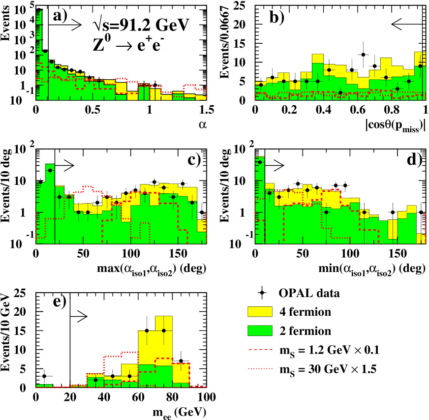
Figure 1: Cut variables for $\mathrm{Z}^{0}\to\mathrm{e}^{+}\mathrm{e}^{-}$ at $\sqrt{s}$ = 91.2 GeV. The OPAL data are indicated by dots with error bars (statistical error), the four-fermion background by the light grey histograms and the two-fermion background by the medium grey histograms. The signal distributions from a 1.2 GeV $\mathrm{S}^{0}$ are plotted as dashed lines and those from a 30 GeV $\mathrm{S}^{0}$ as dotted lines, respectively. The signal histograms are normalised corresponding to 0.1 and 1.5 times of the Standard Model Higgs-strahlung cross section and show the decay channel $\mathrm{S}^{0}\to\mathrm{gg}$. Each variable is shown with the cuts applied before the cut on this variable is done, respecting the order of cuts in Table 3. The arrows indicate the accepted regions. The histograms in Figure a) have non-constant bin widths.

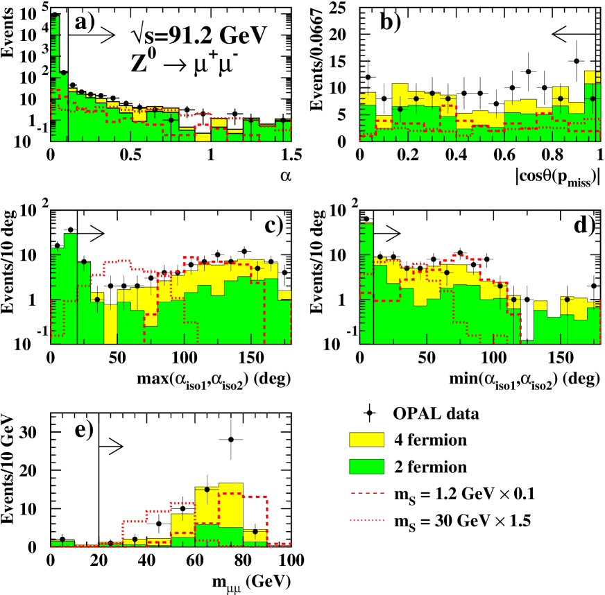
Figure 2: Cut variables for $\mathrm{Z}^{0}\to\mu^{+}\mu^{-}$ at $\sqrt{s}$ = 91.2 GeV. The OPAL data are indicated by dots with error bars (statistical error), the four-fermion background by the light grey histograms and the two-fermion background by the medium grey histograms. The signal distributions from a 1.2 GeV $\mathrm{S}^{0}$ are plotted as dashed lines and those from a 30 GeV $\mathrm{S}^{0}$ as dotted lines, respectively. The signal histograms are normalised corresponding to 0.1 and 1.5 times of the Standard Model Higgs-strahlung cross section and show the decay channel $\mathrm{S}^{0}\to\mathrm{gg}$. Each variable is shown with the cuts applied before the cut on this variable is done, respecting the order of cuts in Table 3. The arrows indicate the accepted regions. The histograms in Figure a) have non-constant bin widths.

All cuts are listed in Table 2 and the number of events after each cut is given in Table 3. The distributions of the cut variables in data and Monte Carlo are shown in Figures 1 and 2. After the selection 45 events remain in the channel $\mathrm{Z}^{0}\to\mathrm{e}^{+}\mathrm{e}^{-}$, with  $\mathrm{55.2}\pm\mathrm{3.0\,(stat.)}\pm\mathrm{3.0\,(syst.)}$ events expected from SM background (the evaluation of the systematic uncertainties is described in section 4.1.4). In the channel $\mathrm{Z}^{0}\to\mu^{+}\mu^{-}$, 66 events remain in the data with  $\mathrm{53.6}\pm\mathrm{2.7\,(stat.)}\pm\mathrm{2.1\,(syst.)}$ expected from SM background.

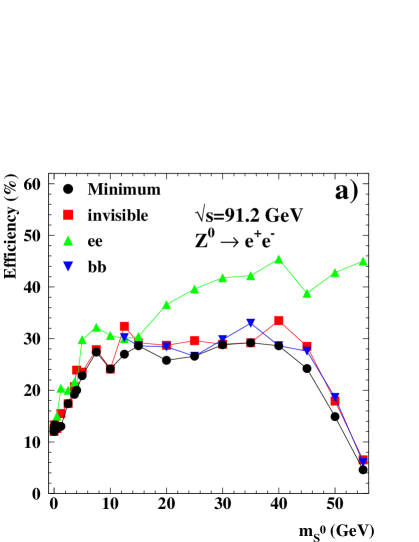
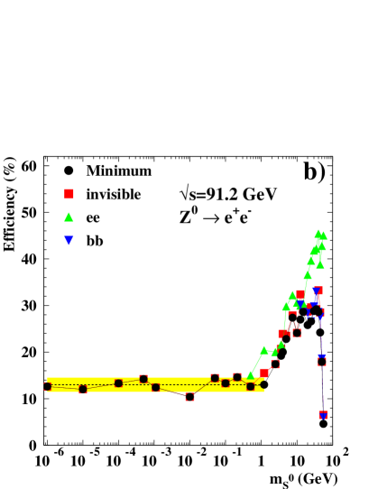
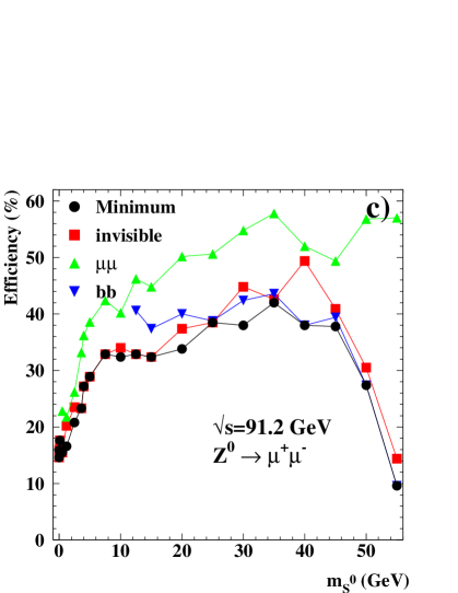
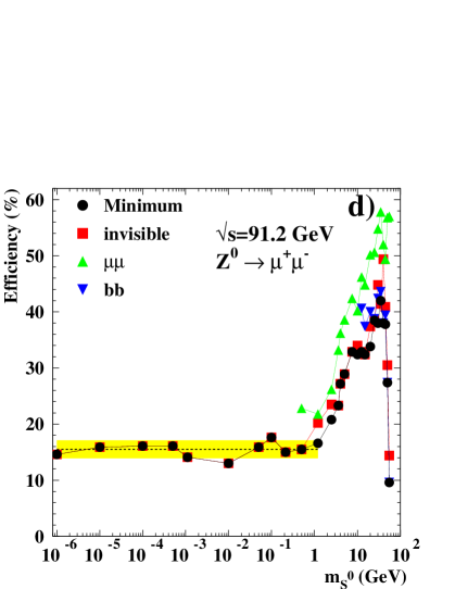
Figure 3: The efficiency versus the $\mathrm{S}^{0}$ mass at $\sqrt{s}=91.2$ GeV for a subset of decay modes of $\mathrm{S}^{0}$: a)+b) $\mathrm{Z}^{0}\to\mathrm{e}^{+}\mathrm{e}^{-}$ in linear and logarithmic mass scale; c)+d) $\mathrm{Z}^{0}\to\mu^{+}\mu^{-}$ in linear and logarithmic mass scale. The minimum efficiencies which are used in the limits are also shown. In the low mass region, below the threshold for the decays of the $\mathrm{S}^{0}$ into a pair of SM fermions, only the decays into photons or invisible particles are possible. For $m_{\mathrm{S}^{0}}\lesssim\Gamma_{\mathrm{Z}^{0}}$ the efficiency is almost flat. This is indicated by the dashed line which marks the average efficiency for $m_{\mathrm{S}^{0}}\leq 1$ GeV. The shaded bands show the typical error on the efficiencies in this region.

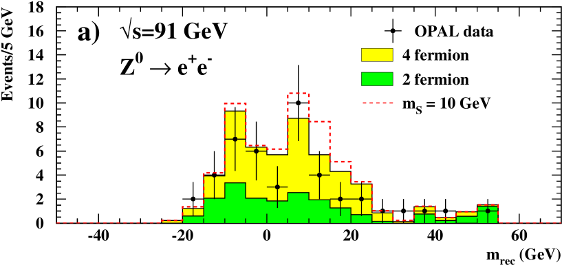
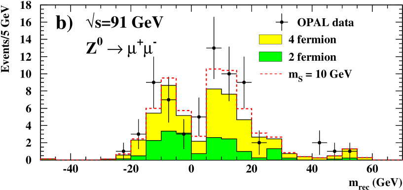
Figure 4: The recoil mass spectra from $\sqrt{s}=$91.2 GeV a) for the decays $\mathrm{Z}^{0}\to\mathrm{e}^{+}\mathrm{e}^{-}$ and b) for $\mathrm{Z}^{0}\to\mu^{+}\mu^{-}$. OPAL data are indicated by dots with error bars (statistical error), the four-fermion background by the light grey histograms and the two-fermion background by the dark grey histograms. The dashed lines for the signal distributions are plotted on top of the background distributions with normalisation corresponding to the cross section excluded at 95% confidence level from the combination of both channels.

Figure 3 shows the efficiency versus the $\mathrm{S}^{0}$ mass for some example decay modes. The signal efficiency is at least 20% in the electron channel and at least 27% in the muon channel for $\mathrm{S}^{0}$ masses between 4 and 45 GeV. At masses below the kinematic threshold for the decay of the $\mathrm{S}^{0}$ into $\mathrm{e}^{+}\mathrm{e}^{-}$ ($\sim 1~{}\mbox{MeV}$) only decays into photons or invisible particles are possible. For each $\mathrm{S}^{0}$ mass hypothesis the smallest efficiency of all decay channels studied (also shown in Figure 3) is used in the limit calculation. The analysis is sensitive to a large range of $\mathrm{S}^{0}$ masses, down to masses $m_{\mathrm{S}^{0}}$ well below $\Gamma_{\mathrm{Z}^{0}}$, where the cross section increases significantly. For this mass range mainly soft bosons $\mathrm{S}^{0}$ with energy $E_{\mathrm{S}^{0}}<\Gamma{{}_{\mathrm{Z}}^{0}}$ are emitted, but the spectrum exhibits a significant tail to large energies, which yields a detectable event topology. Figure 4 shows the recoil mass spectrum to the $\mathrm{Z}^{0}$ decay products for both channels at $\sqrt{s}$ = 91.2 GeV. The recoil mass squared is calculated from

$$m_{\mathrm{rec}}^{2}=\left(\sqrt{s}-E_{\ell\ell}\right)^{2}-p_{\ell\ell}^{2},$$ (6)

where $E_{\ell\ell}$ and $p_{\ell\ell}$ are the energy and the momentum sum of the two lepton tracks, and $\sqrt{s}$ is the centre-of-mass energy. The momentum sum is calculated from the track momentum of the $\mathrm{Z}^{0}$ decay products in the muon channel and from the track momentum and energy deposition of the electrons in the electromagnetic calorimeter in the electron channel.

4.1.2 Cuts used only in the LEP 2 selection

In the analysis for LEP 2 energies, signal and background characteristics differ significantly from those at LEP 1.

• The most important difference compared to the LEP 1 analysis is the fact that in signal processes an on-shell $\mathrm{Z}^{0}$ boson is produced. The selection requires the invariant mass $m_{\ell\ell}$ of the lepton pair to be consistent with the $\mathrm{Z}^{0}$ mass. Due to the limited detector mass resolution, invariant masses within $m_{\mathrm{Z}^{0}}\pm 8~{}\mbox{GeV}$ and $m_{\mathrm{Z}^{0}}\pm 10~{}\mbox{GeV}$ are accepted for the electron and the muon channel, respectively.

• The dominant background at this stage originates from leptonic $\mathrm{Z}^{0}$ decays with photon radiation in the initial state. At centre-of-mass energies above $m_{\mathrm{Z}^{0}}$ the cross section for radiating one (or more) high energy initial-state photon(s) is enhanced if the effective centre-of-mass energy of the electron-positron pair after photon emission is close to the $\mathrm{Z}^{0}$ mass. Such events are called ‘radiative returns’ to the $\mathrm{Z}^{0}$ pole. These background events are characterised by an acolinear and sometimes acoplanar lepton pair and one or more high energy photons. Such events are rejected by a $\gamma$-veto: if there is only one cluster in the electromagnetic calorimeter not associated to a track and the energy $E_{\mathrm{unass}}$ of the cluster exceeds 60 GeV, then the event is rejected. Events with two tracks and more than 3 GeV energy deposition in the forward calorimeters (covering the polar angle region 47–200 mrad) are also vetoed. The cross section for two fermion production is much smaller at LEP 2 than at LEP 1 so events with final state radiation are not such an important background as in the LEP 1 case.

• In the remaining background from two-photon processes and $(\mathrm{Z}/\gamma)^{*}\to\mathrm{e}^{+}\mathrm{e}^{-},\mu^{+}\mu^{-}$ with initial-state radiation the leptons carry considerable momentum along the beam axis. We reject these events by requiring $|p^{z}_{1}+p^{z}_{2}|<50~{}\mbox{GeV}$ where $p^{z}_{i}$ are the $z$-components of the momentum of the two lepton candidates.

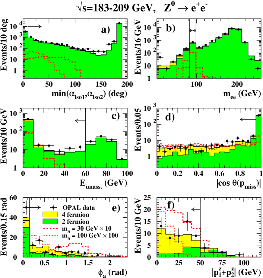
Figure 5: Cut variables for $\mathrm{Z}^{0}\to\mathrm{e}^{+}\mathrm{e}^{-}$ at $\sqrt{s}=183$–$209~{}\mbox{GeV}$. The OPAL data are indicated by dots with error bars (statistical error), the four-fermion background by the light grey histograms and the two-fermion background by the medium grey histograms. The signal distributions from a 30 GeV $\mathrm{S}^{0}$ are plotted as dashed lines and those from a 100 GeV $\mathrm{S}^{0}$ as dotted lines, respectively. The signal histograms are normalised to 10 and 100 times of the Standard Model Higgs-strahlung cross section, respectively, and show the decays $\mathrm{S}^{0}\to\mathrm{gg}$. Each variable is shown with the cuts applied before the cut on this variable is done, respecting the order of cuts in Table 4. The arrows indicate the accepted regions.

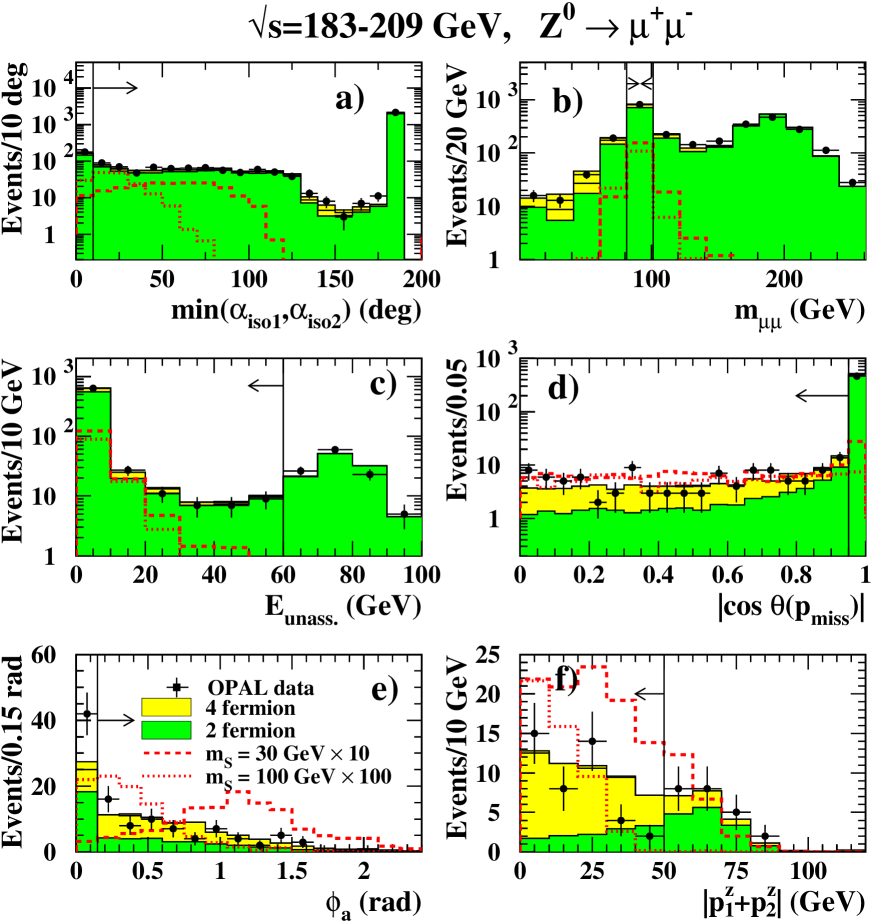
Figure 6: Cut variables for $\mathrm{Z}^{0}\to\mu^{+}\mu^{-}$ at $\sqrt{s}=183$–$209~{}\mbox{GeV}$. The OPAL data are indicated by dots with error bars (statistical error), the four-fermion background by the light grey histograms and the two-fermion background by the medium grey histograms. The signal distributions from a 30 GeV $\mathrm{S}^{0}$ are plotted as dashed lines and those from a 100 GeV $\mathrm{S}^{0}$ as dotted lines, respectively. The signal histograms are normalised to 10 and 100 times of the Standard Model Higgs-strahlung cross section, respectively, and show the decays $\mathrm{S}^{0}\to\mathrm{gg}$. Each variable is shown with the cuts applied before the cut on this variable is done, respecting the order of cuts in Table 4. The arrows indicate the accepted regions.

All cuts are listed in Table 2 and the number of events after each cut is given in Table 4. The distributions of the cut variables in data and Monte Carlo are shown in Figures 5 and 6 for data taken at $\sqrt{s}$= 183–209 GeV. A total of 54 events remain in the data of 183–209 GeV in the channel $\mathrm{Z}^{0}\to\mathrm{e}^{+}\mathrm{e}^{-}$, with  $\mathrm{46.9}\pm\mathrm{0.6\,(stat.)}\pm\mathrm{3.3\,(syst.)}$ events expected from SM background (the evaluation of the systematic uncertainties is described in section 4.1.4). In the channel $\mathrm{Z}^{0}\to\mu^{+}\mu^{-}$, 43 events remain in the data with  $\mathrm{51.6}\pm\mathrm{0.3\,(stat.)}\pm\mathrm{2.6\,(syst.)}$ expected from SM background. The signal efficiency is at least 24% in the electron channel and at least 30% in the muon channel for $\mathrm{S}^{0}$ masses between 30 and 90 GeV.

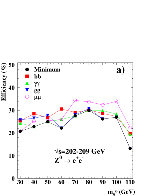
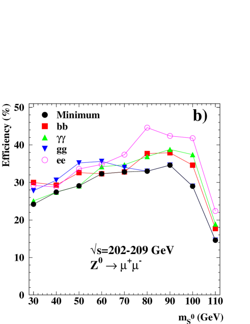
Figure 7: The efficiency versus the $\mathrm{S}^{0}$ mass at $\sqrt{s}=202$–$209$ GeV for a subset of decay modes of $\mathrm{S}^{0}$ a) in the $\mathrm{Z}^{0}\to\mathrm{e}^{+}\mathrm{e}^{-}$ and b) $\mathrm{Z}^{0}\to\mu^{+}\mu^{-}$ channel. The minimum efficiencies which are used in the limits are given as well. For the other LEP 2 centre-of-mass energies the signal efficiencies are similar.

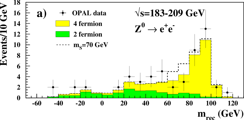
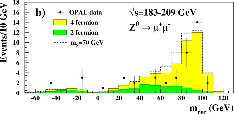
Figure 8: The recoil mass spectrum from 183–209 GeV a) for the decays $\mathrm{Z}^{0}\to\mathrm{e}^{+}\mathrm{e}^{-}$ and b) for $\mathrm{Z}^{0}\to\mu^{+}\mu^{-}$ (lower plot). OPAL data are indicated by dots with error bars (statistical error), the four-fermion background by the light grey histograms and the two-fermion background by the medium grey histograms. The dashed lines for the signal distributions are plotted on top of the background distributions with normalisation corresponding to the excluded cross section from the combination of both channels.

Figure 7 shows the efficiency versus the $\mathrm{S}^{0}$ mass at $\sqrt{s}=202$–$209~{}\mbox{GeV}$ for some example decays as well as the minimum efficiencies which are used in the limit calculation. The efficiencies for 183–202 GeV have similar values for $m_{\mathrm{S}^{0}}<100~{}\mbox{GeV}$. For the lower centre-of-mass energies the efficiency decreases faster for higher masses due to kinematic effects, primarily the cut on the acoplanarity angle. Figure 8 shows the recoil mass spectrum for both channels summed from 183–209 GeV.

4.1.3 Correction on background and signal efficiencies

In all channels a correction is applied to the number of expected background events and the signal efficiencies due to noise in the detectors in the forward region which is not modelled by the Monte Carlo. The correction factor is derived from the study of random beam crossings. The fraction of events that fail the veto on activity in the forward region is 7.5 % for LEP 1 and 3.1 % for LEP 2. Since the veto is applied only to events with less than or equal to four tracks, the corrections on the expected background in the actual analyses are typically only 1.8–3.5 %. For the signal efficiencies the full correction is applied to the decay channels where appropriate.

4.1.4 Systematic uncertainties

The systematic uncertainty of the lepton identification efficiency is studied in a control sample of events with two collinear tracks of which at least one is tagged as an electron or muon. The systematic uncertainty is obtained from the difference of the identification efficiencies for the other track between data and Monte Carlo.

The tracking systematics are studied by changing the track resolution in the Monte Carlo by a relative fraction of 5% in $d_{0}$ and $\phi$ and by 10% in $z_{0},\kappa$ and $\cot\theta$, which corresponds to the typical difference in the resolution of these parameters in data and Monte Carlo. The difference in signal and background expectation compared to the one obtained from the unchanged track resolution is taken as the systematic uncertainty.

The reconstruction of the energy deposition in the electromagnetic calorimeter and the momentum in the tracking system of the lepton candidates is investigated with the help of the mean values $\bar{x}_{dat}$ and $\bar{x}_{MC}$ of the distributions of $p$ and $E$ from the collinear lepton pair control sample for data and Monte Carlo expectation. The analyses are repeated with the cuts on $p$ and $E$ being changed by the difference $|\bar{x}_{dat}-\bar{x}_{MC}|$. The deviations in the number of expected events compared to the original cuts are taken as the systematic uncertainties.

The uncertainty from the lepton isolation angle $\alpha_{\mathrm{iso}}$ is studied in different ways for the LEP 1 and LEP 2 analysis. In the LEP 1 selection a control sample of hadronic events is selected. Random directions are then chosen in the event, and the angles $\alpha_{\mathrm{iso}}$ of the vectors pointing to these directions are determined. The cut on $\alpha_{\mathrm{iso}}$ is varied by the difference of the mean of the data and the Monte Carlo distributions of the control sample. In the LEP 2 selection the uncertainty is obtained in a similar way but from the isolation of the lepton in W⁺W${}^{-}\to\mathrm{q\bar{q}}\ell\nu$ events.

Correct modelling of photon radiation and conversions is a crucial ingredient of the decay-mode independent searches. For LEP 1, the effect of the description of photon radiation in the Monte Carlo is estimated from the difference in the number of events between data and background expectation after removing the photon and conversion veto. At least one identified photon or conversion is required for the tested events. In the muon channel at LEP 2 energies two different Monte Carlo generators are used for the two-fermion background, and the difference between the background prediction of the two generators is taken as the systematic uncertainty of the photon modelling. For the electron channel only one generator is available. Here, the uncertainty is determined from the comparison of the number of events in the data and Monte Carlo sets in a side band of the distribution of the lepton pair invariant mass where no signal is expected. This test is dominated by the statistical uncertainties of the side-band sub-sample.

In the analysis the four-fermion Monte Carlo samples are reweighted to account for low mass resonances (e.g. $\rho,\omega,\phi,J/\psi$) and the running of $\alpha_{\mathrm{em}}(q^{2})$. The uncertainty from this reweighting is assessed to be 50% of the change of the expected background after switching off the reweighting.

All uncertainties for a particular centre-of-mass energy are assumed to be uncorrelated and the individual contributions are added in quadrature for the total systematic uncertainty. The dominant systematic uncertainties in the LEP 1 background expectation come from the description of photon radiation and photon conversions in the Monte Carlo as well as from the uncertainty of the four-fermion cross section. The precision of the predicted signal efficiency is mainly limited by the description of the lepton isolation.

In the LEP 2 selection the modelling of the radiative returns has a large impact on the total systematic uncertainty, both in the electron and the muon channel. In the electron channel the uncertainty from the isolation angle criterion and in the muon channel the uncertainty of the muon identification efficiency are also significant.

For the LEP 2 data, the evaluation of the systematic uncertainties at each single centre-of-mass energy is limited by Monte Carlo statistics. Therefore they are investigated for the total set of Monte Carlo samples with $\sqrt{s}=183$–$209~{}\mbox{GeV}$.

The numbers of expected background events for the LEP 1 and LEP 2 analyses, broken down by the different centre-of-mass energies, are listed in Table 5 for the channels $\mathrm{Z}^{0}\to\mathrm{e}^{+}\mathrm{e}^{-}$ and $\mathrm{Z}^{0}\to\mu^{+}\mu^{-}$. The numbers include systematic errors discussed above and the statistical error from the limited Monte Carlo samples. Also the number of expected events from a 30 GeV Standard Model Higgs boson is shown. A detailed overview of the different systematic uncertainties is given in Table 6.

4.2 Event selection for $\mathrm{e}^{+}\mathrm{e}^{-}$ $\to$ S⁰Z${}^{0}\to$ $n\cdot\gamma\,\nu\overline{\nu}$, $\mathrm{e}^{+}\mathrm{e}^{-}\nu\overline{\nu}$

In this section a search for $\mathrm{e}^{+}\mathrm{e}^{-}$ $\to$ S⁰Z${}^{0}\to$ $n\cdot\gamma\,\nu\overline{\nu}$ or $\mathrm{e}^{+}\mathrm{e}^{-}\nu\overline{\nu}$ (the latter for $m_{\mathrm{S}^{0}}<500~{}\mbox{MeV}$) at $\sqrt{s}=91.2~{}\mbox{GeV}$ is described. The removal of radiative backgrounds in the selection described in section 4.1.1 rejects the $\mathrm{S}^{0}$ decays into photons (due to the photon veto) and, in the mass region $m_{\mathrm{S}^{0}}<500~{}\mbox{MeV}$, also the decays into electrons (due to the conversion veto). The selection for S⁰Z${}^{0}\to$ S⁰$\nu\overline{\nu}$ is included to recuperate the sensitivity to the photon and electron decay modes and therefore to remain decay-mode independent.

4.2.1 Event selection

In signal events the $\mathrm{S}^{0}$ is radiated off the $\mathrm{Z}^{0}$ with some kinetic energy and a certain amount of transverse momentum. Therefore the total visible energy $E_{\mathrm{vis}}$ in the electromagnetic calorimeter is required to exceed 12 GeV and the transverse momentum $p_{T}$ reconstructed from the event is required to exceed 6 GeV. Since the $\mathrm{Z}^{0}$ decays into neutrinos which carry energy out of the detector, the total amount of visible energy is reduced. The selection requires $E_{\mathrm{vis}}<60~{}\mbox{GeV}$.

Several cuts are applied to reduce the background from processes with topologies different from the signal. The selection allows only events with zero ($n\cdot\gamma\,\nu\overline{\nu}$-channel) or two ($\mathrm{e}^{+}\mathrm{e}^{-}$ $\nu\overline{\nu}$-channel) identified electrons, using the same electron identification routines as described in section 4.1. The next selection cuts are intended to further reduce background from cosmic rays or beam halo particles. Events triggered by cosmic rays or beam halo particles are characterised by extended clusters in the electromagnetic calorimeter, hits in the hadron calorimeter and muon chambers and a signal from the time-of-flight counter that shows a significant discrepancy from its expected value. We therefore require no hit in the muon chambers and at most two hits in the hadron calorimeter. No more than one cluster with an energy deposition larger than 2 GeV is allowed in the hadron calorimeter. The number of lead glass blocks in each cluster in the electromagnetic calorimeter must be less than 15. The difference between the measured time of flight and the expected time for a particle coming from the interaction point is required to be less than 2 ns.

The remaining background is mostly from $\mathrm{e}^{+}\mathrm{e}^{-}\to\nu\bar{\nu}\gamma$ events, where the photon is usually emitted at small angles to the beam axis. A hard cut on the angular distribution of clusters in the electromagnetic calorimeter and the forward calorimeters (polar angle region 47–200 mrad) is applied. For this purpose the polar angle of the energy vector $\vec{E}$ is defined as

$$\theta_{\vec{E}}=\sum_{i=1,n}\frac{E_{i}\cdot\theta_{i}}{E_{\mathrm{vis}}}.$$

The sum runs over all clusters $i$ (with polar angle $\theta_{i}$). Cuts applied on the energy vector and the individual clusters are $|\cos\theta_{\vec{E}}|<0.65$ and $|\cos\theta_{i}|<0.9$. The energy in the forward calorimeters must be less than 2 GeV.

Events with two electrons must satisfy some additional requirements. The tracks must be identified as electrons with opposite charge. The angle $\Delta\phi$ between the tracks must be less than $\mathrm{10}^{\circ}$, the invariant mass $m_{\ell\ell}$ must be less than 2 GeV, and a transverse momentum $p_{T}>7~{}\mbox{GeV}$ of the event is required. Events are rejected if there are any additional clusters other than those associated with one of the two tracks.

A correction due to random detector occupancy is applied as described in section 4.1.3. The full correction of $-7.5\,\%$ is used since the forward detector veto applies to all events.

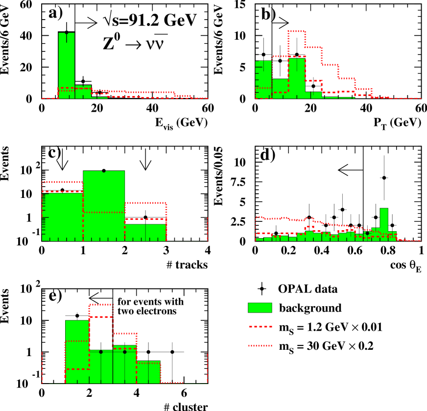
Figure 9: Some of the cut variables for $\mathrm{Z}^{0}\to\nu\bar{\nu}$ at $\sqrt{s}$ = 91.2 GeV. The last plot (number of clusters) is one of the additional cut variables which are used in events with two electrons. The OPAL data are indicated by dots with error bars (statistical error), and the total background by the grey histograms. The distributions from a 1.2 GeV and a 30 GeV signal are plotted as dashed and dotted lines, respectively. The signal histograms are normalised corresponding to 0.01 times and 0.2 times the Standard Model Higgs-strahlung cross section and show the decay channel $\mathrm{S}^{0}\to\gamma\gamma$. Each variable is shown with all cuts but the cut on the variable itself. The arrows indicate the accepted regions.

After all cuts 15 events are selected from the data with a background prediction of $11.3\pm 1.1({\mathrm{stat.}})\pm 0.2({\mathrm{syst.}})$, where the uncertainties are evaluated as described below. Figure 9 shows the distribution of the cut variables in data and Monte Carlo.

There is no statistically significant excess in this channel, and the shape of the distributions of the cut variables in data and Monte Carlo are in good agreement. Furthermore the product of the signal efficiency and the $\mathrm{Z}^{0}\to\nu\overline{\nu}$ decay branching ratio is substantially higher than for the $\mathrm{S}^{0}$ $\ell^{+}\ell^{-}$-channels, and the predicted background is much less. Hence, the channel $\mathrm{Z}^{0}\to\nu\overline{\nu}$ has much higher sensitivity than the electron and the muon channel. It does not contribute to the actual limits, provided that the systematic uncertainties are not much larger than in the other channels. For a conservative limit calculation only the channels with lowest sensitivity are used.

The search channel described in this section recovers sensitivity to the decay modes $\mathrm{S}^{0}\to n\cdot\gamma$ and at low masses $m_{\mathrm{S}^{0}}$ to the decay $\mathrm{S}^{0}\to\mathrm{e}^{+}\mathrm{e}^{-}$ to which the analysis described in section 4.1.1 had no sensitivity. However, the requirement $E_{\mathrm{vis}}>12~{}\mbox{GeV}$ in this channel can lead to an insensitivity to decays $\mathrm{S}^{0}\to\chi^{0}_{2}\chi^{0}_{1}\to\gamma\chi^{0}_{1}\chi^{0}_{1}$ for certain combinations of $m_{\mathrm{S}^{0}},m_{\chi^{0}_{2}}$ and $m_{\chi^{0}_{1}}$ for the whole LEP 1 analysis.

4.2.2 Systematic uncertainties

Uncertainties in this channel predominantly come from the energy calibration of the electromagnetic calorimeters. In reference [21] it is shown that an electromagnetic cluster has a calibration uncertainty of 25 MeV. Since the number of clusters in the electromagnetic calorimeter for selected data and Monte Carlo events is less than five, the deviation of the expected number of background events and the signal efficiencies after shifting the cuts on the visible energy $E_{\mathrm{vis}}$ and the transverse momentum $p_{T}$ by four times 25 MeV is used as a systematic uncertainty. The deviation is found to be 1.4 %. From the same reference [21] we take the systematic uncertainties on the time-of-flight signal (0.5 %). Other sources for systematic uncertainties are the luminosity (0.5 %), the limited Monte Carlo statistics (10.0 % for background and 2.2 % for the signal) and, for events where the $\mathrm{S}^{0}$ decays into electrons, the uncertainty on the electron identification efficiency (0.8 %). Summing these individual sources up in quadrature, estimates of the total uncertainty in the background of 10.0 %(stat.)$+$1.8 %(syst.) and in the signal of 2.2 %(stat.)$+$1.6 %(syst.) are obtained. Given the expected number of signal and background events, this is much less than the level where the channel starts contributing to the limit calculation.

5 Results

The results of the decay-mode independent searches are summarised in Table 5, which compares the numbers of observed candidates with the background expectations. The total number of observed candidates from all channels combined is 208, while the Standard Model background expectation amounts to $207.3\pm 4.1(\mathrm{stat.})\pm 11.1(\mathrm{syst.})$. For each individual search channel there is good agreement between the expected background events and observed candidates. As no significant excess over the expected background is observed in the data, limits on the cross section for the Bjorken process $\mathrm{e}^{+}\mathrm{e}^{-}\to$ $\mathrm{S}^{0}$$\mathrm{Z}^{0}$ are calculated.

The limits are presented in terms of a scale factor $k$, which relates the cross section for $\mathrm{S}^{0}$$\mathrm{Z}^{0}$ to the Standard Model one for the Higgs-strahlung process $\mathrm{e}^{+}\mathrm{e}^{-}\to$ $\mathrm{H}^{0}_{\mathrm{SM}}$$\mathrm{Z}^{0}$ as defined in Equation 1. The 95% CL upper bound on $k$ is obtained from a test statistic for the signal hypothesis, by using the weighted event-counting method described in [22]: In each search channel, given by the different centre-of-mass energies and the $\mathrm{Z}^{0}$ decay modes considered, the observed recoil mass spectrum is compared to the spectra of the background and the signal. The latter is normalised to $\varepsilon\cdot\mathrm{BR}\cdot{\cal{L}}\cdot k\cdot\sigma_{\mathrm{\mathrm{H}^{0}\mathrm{Z}^{0}}}$, where $\varepsilon$ is the minimum signal detection efficiency out of all tested decay modes, BR is the branching ratio of the $\mathrm{Z}^{0}$ decay mode considered in this channel and $\cal{L}$ is the integrated luminosity recorded for that channel. The efficiencies for arbitrary $\mathrm{S}^{0}$ masses are interpolated from the efficiencies at masses for which Monte Carlo samples were generated. Every event in each of these mass spectra and each search channel is given a weight depending on its expected ratio of signal over background, $s/b$, at the given recoil mass. For every assumed signal $\mathrm{S}^{0}$ mass these weights are a function of the signal cross section, which is taken to be $k$ times the Standard Model Higgs cross section for the same $\mathrm{S}^{0}$ mass. Finally, from the sum of weights for the observed number of events, an upper limit $k^{95}$ for the scale factor is determined at the 95% confidence level.

The systematic uncertainties on the background expectations and signal selection efficiencies are incorporated using the method described in [23].

The limits are given for three different scenarios:

1. Production of a single new scalar S⁰.

2. The Uniform Higgs scenario.

3. The Stealthy Higgs scenario.

5.1 Production of a single new scalar S⁰

In the most general interpretation of our results, a cross-section limit is set on the production of a new neutral scalar boson $\mathrm{S}^{0}$ in association with a $\mathrm{Z}^{0}$ boson. To calculate the limit we use the mass distributions of which the sums are shown in Figure 4 and 8 for OPAL data, the expected background and the signal.

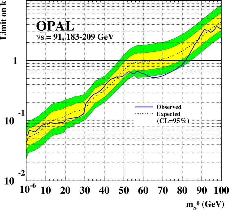
Figure 11: The upper limit on the scale factor $k$ on the cross section for the production of a new scalar boson in the Higgs-strahlung-process (solid line). The dot-dashed line represents the expected median for background-only experiments. Both limits are calculated at the 95 % confidence level. The dark (light) shaded bands indicate the 68% (95%) probability intervals centred on the median expected values. For masses $m_{\mathrm{S}^{0}}\lesssim 1~{}\mbox{GeV}$ the limits are constant. The lowest signal mass tested is $10^{-6}~{}\mbox{GeV}$.

In Figure 11 we present the limits obtained for scalar masses down to the lowest generated signal mass of 1 keV. They are valid for the decays of the $\mathrm{S}^{0}$ into hadrons, leptons, photons and invisible particles (which may decay inside the detector) as well as for the case in which the $\mathrm{S}^{0}$ has a sufficiently long lifetime to escape the detector without interacting or decaying. A decay of the $\mathrm{S}^{0}$ into invisible particles plus photons, however, can lead to a reduced sensitivity in the mass region where the sensitivity of the analyses is dominated by the LEP 1 data (see section 4.2.1). The observed limits are given by the solid line, while the expected sensitivity, determined from a large number of Monte Carlo experiments with only background, is indicated by the dotted line. The shaded bands indicate the one and two sigma deviations from the expected sensitivity. Values of $k>0.1$ are excluded for values of $m_{\mathrm{S}^{0}}$ below 19 GeV, whereas $k>1$ is excluded from the data for $m_{\mathrm{S}^{0}}$ up to 81 GeV, independent of the decay modes of the $\mathrm{S}^{0}$ boson. This means that the existence of a Higgs boson produced at the SM rate can be excluded up to this mass even from decay-mode independent searches. For masses of the new scalar particle well below the width of the $\mathrm{Z}^{0}$, i.e. $m_{\mathrm{S}^{0}}\lesssim 1~{}\mbox{GeV}$, the obtained limits remain constant at the level of $k^{95}_{\mathrm{obs.}}=0.067$, and $k^{95}_{\mathrm{exp.}}=0.051$.

The discrepancy between the expected and the observed limits is within one standard deviation for masses below 52 GeV and for masses above 82 GeV. The deviation of about two sigma in the mass range 52–82 GeV is due to a deficit of selected data events in the recoil mass spectrum of both the electron and muon channels.

5.2 Limits on signal mass continua

5.2.1 The Uniform Higgs scenario

We simulated signal spectra for the Uniform Higgs scenario for $\tilde{K}=\mathrm{constant}$ over the interval [$m_{\mathrm{A}}$, $m_{\mathrm{B}}$] and zero elsewhere. Both the lower mass bound $m_{\mathrm{A}}$ and the upper bound $m_{\mathrm{B}}$ are varied between 1 GeV and 350 GeV (with the constraint $m_{\mathrm{A}}\leq m_{\mathrm{B}}$). In a similar way to the previous section we get an upper limit on the integral in Equation 2.

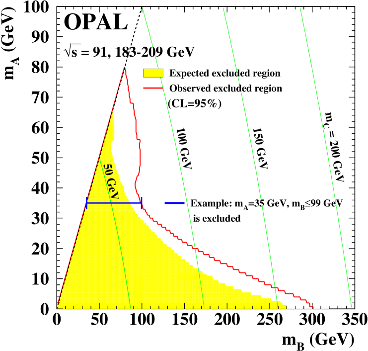
Figure 12: Exclusion limits for the Uniform Higgs scenario at the 95 % confidence level. All mass intervals ($m_{\mathrm{A}}$, $m_{\mathrm{B}}$) within the area bordered by the dark line are excluded from the data. The shaded area marks the mass points which are expected to be excluded if there were only background. The light grey curves indicate isolines for several values of $m_{\mathrm{C}}$. All intervals $(m_{\mathrm{A}},m_{\mathrm{B}})$ to the right of each isoline are theoretically disallowed from Equation 3. By definition, only intervals $(m_{\mathrm{A}},m_{\mathrm{B}})$ right to the dashed diagonal line are valid, i.e. $m_{\mathrm{A}}\leq m_{\mathrm{B}}$.

Figure 12 shows the mass points ($m_{\mathrm{A}}$,$m_{\mathrm{B}}$) for which the obtained 95 % CL limit on $\int\mathrm{d}m\,\tilde{K}$ is less than one. These are the signal mass ranges $m_{\mathrm{A}}\leq m_{\mathrm{h^{0}_{i}}}\leq m_{\mathrm{B}}$ which can be excluded assuming a constant $\tilde{K}$.

If $m_{\mathrm{A}}=m_{\mathrm{B}}$, then the signal spectrum reduces to the mass distribution of a single boson. Excluded points on the diagonal $m_{\mathrm{A}}=m_{\mathrm{B}}$ are therefore the same masses as in Figure 11 for which $k<1$. The horizontal line illustrates an example for excluded mass ranges: The line starts on the diagonal at $m_{\mathrm{A}}=m_{\mathrm{B}}=35~{}\mbox{GeV}$ and ends at $m_{\mathrm{B}}=99~{}\mbox{GeV}$. This value of $m_{\mathrm{B}}$ is the highest upper mass bound which can be excluded for this value of $m_{\mathrm{A}}$. All mass ranges with an upper bound $m_{\mathrm{B}}$ below 99 GeV are also excluded for $m_{\mathrm{A}}=35~{}\mbox{GeV}$. The highest excluded value of $m_{\mathrm{B}}$ ($m_{\mathrm{B}}=301~{}\mbox{GeV})$ is achieved for $m_{\mathrm{A}}$ set to 0 GeV.

Using the two sum rules from section 2.1, lower limits on the perturbative mass scale $m_{\mathrm{C}}$ can be derived. For each excluded value of $m_{\mathrm{A}}$ we take the highest excluded value of $m_{\mathrm{B}}$ and determine the lower bound of $m_{\mathrm{C}}$ according to Equation 3. The excluded mass ranges for $m_{\mathrm{C}}$, assuming a constant $\tilde{K}$, are shown in Figure 13.

5.2.2 Bin-by-bin limits

The limits presented in section 5.2.1 are specific to the case where the coupling density is constant in the interval [$m_{\mathrm{A}}$, $m_{\mathrm{B}}$] and zero elsewhere. The data can also be used to exclude other forms of $\tilde{K}(m)$. To provide practical information for such tests, we have measured $\tilde{K}(m)$ in mass bins with a width comparable to the experimental mass resolution. The typical resolution of the recoil mass in the LEP 1 analysis varies between 1 and 5 GeV in the mass region between 10 and 55 GeV. In the LEP 2 analysis the width is between 3 and 15 GeV for recoil masses between 20 and 100 GeV. The width gets smaller at higher recoil masses. The results of the measurement of $\tilde{K}(m)$ are given in Table 7 together with the corresponding statistical and systematic uncertainties.

From these measured numbers of $\tilde{K}(m)$, one can obtain upper limits on the integral $\int\mathrm{d}m\,\tilde{K}(m)$ for any assumed shape of $\tilde{K}(m)$ using a simple $\chi^{2}$ fitting procedure. To account for mass resolution effects, we provide a correction matrix (Table 8). To test a certain theory with a distribution of $\tilde{K}(m)$ values in the 10 measured bins from Table 7, written as a vector $\vec{\kappa}=\left(\tilde{K}_{1},\ldots,\tilde{K}_{10}\right)$, the corrected vector $\vec{\kappa}^{\prime}=\hat{C}\vec{\kappa}$ can then be fitted to the measured values. In the fit the systematic uncertainties, which are small compared to the statistical errors, can be assumed to be fully correlated bin-by-bin.

5.2.3 The Stealthy Higgs scenario

To set limits on the Stealthy Higgs scenario we have simulated the spectrum of a Higgs boson with a width according to Equation 5 and Ref. [4].

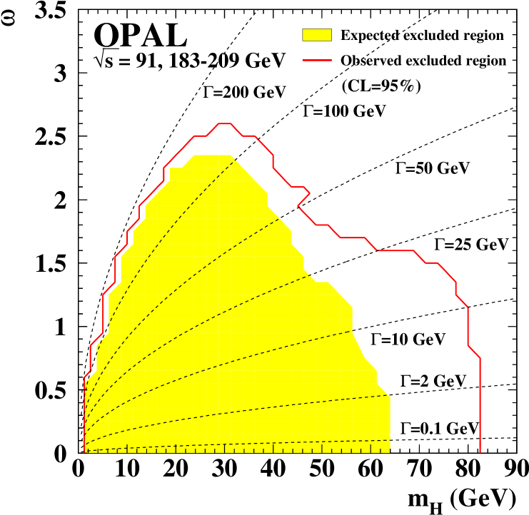
Figure 14: Excluded parameter regions for the simplified Stealthy Higgs scenario at the 95 % confidence level. The solid line marks the region which is excluded from the data. The shaded area marks the region which would be excluded if the data corresponded exactly to the background-only prediction. The dashed lines indicate the Higgs width depending on $m_{\mathrm{H}}$ and $\omega$.

The excluded regions in the $\omega$-$m_{\mathrm{H}}$ parameter space are shown in Figure 14. To illustrate the Higgs width according to Equation 5, for a given mass $m_{\mathrm{H}}$ and coupling $\omega$ ‘isolines’ for some sample widths are added to the plot. The vertical edge in the exclusion contour at $m_{\mathrm{H}}=81~{}(62)~{}\mbox{GeV}$ in the observed (expected) limits reflects the detector mass resolution in $\Delta m$: For a fixed mass $m_{\mathrm{H}}$ the exclusion power is the same for all couplings $\omega$ that yield $\Gamma_{\mathrm{H}}\lesssim\Delta m$, and the limits for $\omega\to 0$ reproduce the limits for a single narrow $\mathrm{S}^{0}$ in Figure 11. The maximal excluded region of the coupling $\omega$ is achieved for masses around 30 GeV, where $\omega$ can be excluded up to $\omega=2.7$. For lower masses the sensitivity drops due to the rapidly increasing width of the Higgs boson, and for higher masses due to the decreasing signal cross section.

6 Conclusions

Searches for new neutral scalar bosons $\mathrm{S}^{0}$ decaying to hadrons of any flavour, to leptons, photons invisible particles and other modes have been performed based on the data collected at $\sqrt{s}$ = $m_{\mathrm{Z}}$ and 183 to 209 GeV by studying the recoil mass spectrum of $\mathrm{Z}^{0}\to\mathrm{e}^{+}\mathrm{e}^{-},\mu^{+}\mu^{-}$ in $\mathrm{S}^{0}$$\mathrm{Z}^{0}$ production and the channel where the $\mathrm{Z}^{0}$ decays into $\nu\overline{\nu}$ and the $\mathrm{S}^{0}$ into photons or $\mathrm{e}^{+}\mathrm{e}^{-}$. No significant excess of candidates in the data over the expected Standard Model background has been observed. Therefore upper limits on the production cross section for associated production of $\mathrm{S}^{0}$ and $\mathrm{Z}^{0}$, with arbitrary $\mathrm{S}^{0}$ decay modes, were set at the 95 % confidence level. Upper limits in units of the Standard Model Higgs-strahlung cross section of $k<0.1$ for $1~{}\mbox{keV}<m_{\mathrm{S}^{0}}<19~{}\mbox{GeV}$ and $k<1$ for $m_{\mathrm{S}^{0}}<81~{}\mbox{GeV}$ were obtained. In further interpretations, limits on broad continuous signal mass shapes to which previous analyses at LEP had no or only little sensitivity were set for the first time. Two general scenarios in the Higgs sector were investigated: A uniform scenario, when the signal arises from many unresolved Higgs bosons, and a Stealthy Higgs model, when the Higgs resonance width is large due to large Higgs-phion couplings.

$\sqrt{s}$ (GeV)	year	integrated luminosity (pb-1)
91.2	1989–95	115.4
183	1997	56.1
189	1998	177.7
192	1999	28.8
196	1999	73.2
200	1999	74.2
202	1999	36.5
202–206	2000	83.1
206–209	2000	132.4

Table 1: Overview of the analysed integrated data luminosities.

LEP 1: $\mathrm{Z}^{0}\to\mathrm{e}^{+}\mathrm{e}^{-},\mu^{+}\mu^{-}$
0.	Preselection	see text
1.	Modified acoplanarity	$0.11~{}\mathrm{rad}<\alpha<2.0~{}\mathrm{rad}$
2.	Polar angle of missing momentum vector	$|\cos\theta(\vec{p}_{\mathrm{miss}})|<0.98\quad$for $p_{\mathrm{miss}}>2~{}\mbox{GeV}$
3.	Isolation of lepton tracks	$\max(\alpha_{\mathrm{iso}_{1}},\alpha_{\mathrm{iso}_{2}})>20^{\circ}$
		$\min(\alpha_{\mathrm{iso}_{1}},\alpha_{\mathrm{iso}_{2}})>10^{\circ}$
4.	Invariant mass of the lepton pair	$20~{}\mbox{GeV}<m_{\ell\ell}<100~{}\mbox{GeV}$
5.	Photon and Conversion veto	see text
LEP 2: $\mathrm{Z}^{0}\to\mathrm{e}^{+}\mathrm{e}^{-},\mu^{+}\mu^{-}$
0.	Preselection	see text
1.	Acoplanarity	$\phi_{a}>$ 0.15–0.20 rad
2.	Polar angle of missing momentum vector	$|\cos\theta(\vec{p}_{\mathrm{miss}})|<0.95\quad$for $p_{\mathrm{miss}}>5~{}\mbox{GeV}$
3.	Isolation of lepton tracks	$\max(\alpha_{\mathrm{iso}_{1}},\alpha_{\mathrm{iso}_{2}})>15^{\circ}$
		$\min(\alpha_{\mathrm{iso}_{1}},\alpha_{\mathrm{iso}_{2}})>10^{\circ}$
4.	Invariant mass of the lepton pair	$|m_{\mathrm{e}^{+}\mathrm{e}^{-}}-m_{\mathrm{Z}^{0}}|<8~{}\mbox{GeV}$
		$|m_{\mu^{+}\mu^{-}}-m_{\mathrm{Z}^{0}}|<10~{}\mbox{GeV}$
5.	Photon veto	see text
6.	Momentum in z-direction	$|p^{z}_{1}+p^{z}_{2}|<$ 50 GeV
LEP 1: $\mathrm{Z}^{0}\to\nu\overline{\nu}$
1.	Cosmic muon and beam halo veto	see text
2.	Number of identified electron tracks	$N_{e}=$ 0 or 2
3.	Visible energy in electromagnetic calorimeter	$E_{\mathrm{Ecal}}>12~{}\mbox{GeV},<60~{}\mbox{GeV}$
4.	Transverse momentum of event	$p_{T}>6~{}\mbox{GeV}$
5.	Direction of energy vector	$|\cos\theta_{\vec{E}}|<0.65$
6.	Energy in forward detector	$E_{\mathrm{Fdet}}<2~{}\mbox{GeV}$
Additional cuts for events with two electron tracks
7.	Angle between tracks	$\Delta\phi<10^{\circ}$
8.	Transverse momentum of event	$p_{T}>7~{}\mbox{GeV}$
9.	Unassociated clusters in electromagnetic calorimeter	$N_{\mathrm{unass.}}=0$

Table 2: A summary of the selection criteria.

$\mbox{$\sqrt{s}$}=91.2~{}\mbox{GeV}$
Cut	Data	Total	2-fermion	4-fermion	2-photon	Signal
		bkg.				($m_{\mathrm{S}^{0}}$=30 GeV)
Electron channel
Preselection	122431	129115	128490	586.3	38.9	46.2 %
$\alpha$	1560	1694	1628	58	8	33.4 %
$|\cos\theta_{p_{\mathrm{miss}}}|$	1500	1628	1571	55	2	32.8 %
Lepton isolation	1368	1466	1414	50	2	28.6 %
$M_{\ell\ell}$	1362	1462	1410	50	2	28.6 %
Photon+Conversion veto	45	55.2	20.5	34.4	0.3	28.6 %
Muon channel
Preselection	109552	115001	114475	459.1	66.6	54.0 %
$\alpha$	1575	1601	1526	58	17	40.2 %
$|\cos\theta_{p_{\mathrm{miss}}}|$	1549	1575	1512	57	6	40.0 %
Lepton isolation	1403	1470	1412	52	6	37.4 %
$M_{\ell\ell}$	1397	1467	1410	51	6	37.4 %
Photon+Conversion veto	66	53.6	17.0	35.4	1.2	35.0 %

Cut	Data	Total	$\nu\bar{\nu}\gamma$	leptons	other	Signal
		bkg.
Missing energy channel
Events with 0 tracks						$m_{\mathrm{S}^{0}}$=5 GeV, $\mathrm{S}^{0}\to\gamma\gamma$
Preselection	73	68.5	63.5	4.8	0.3	44.2 %
$|\cos\theta_{\vec{E}}|<0.65$	54	51.1	48.1	2.7	0.3	38.4 %
$E_{\mathrm{Ecal}}>12~{}\mbox{GeV}$	14	10.7	9.8	0.6	0.3	30.0 %
Events with 2 tracks						$m_{\mathrm{S}^{0}}$=100 MeV, $\mathrm{S}^{0}\to\mathrm{e}^{+}\mathrm{e}^{-}$
Preselection	30	21.6	4.5	11.6	5.5	29.2 %
$|\cos\theta_{\vec{E}}|<0.65$	17	14.4	3.7	9.5	1.2	25.7 %
$\Delta\phi<\mathrm{10}^{\circ}$	13	7.9	3.6	3.7	0.6	25.7 %
$m_{\mathrm{e}^{+}\mathrm{e}^{-}}<2~{}\mbox{GeV}$	12	7.9	3.6	3.7	0.6	25.7 %
Charge $q_{1}\cdot q_{2}=-1$	10	6.3	3.6	2.1	0.6	25.2 %
$N_{unass.}=0$	4	4.0	3.4	0.0	0.6	23.7 %
$p_{T}>7~{}\mbox{GeV}$	3	2.5	2.5	0.0	0.0	20.9 %
$E_{\mathrm{Ecal}}>12~{}\mbox{GeV}$	1	0.5	0.5	0.0	0.0	14.8 %

Table 3: Cutflow tables for the LEP 1 analysis: Number of selected events after each cut. As an example the efficiencies for the signal process with $\mathrm{S}^{0}\to\mathrm{b\overline{b}}$ are given for the lepton channels, and with $\mathrm{S}^{0}\to\gamma\gamma$ and $\mathrm{S}^{0}\to\mathrm{e}^{+}\mathrm{e}^{-}$ for the missing energy channel. The preselection in the missing energy channel includes the cuts 1, 4, 6 from the $\mathrm{Z}^{0}\to\nu\overline{\nu}$ channel in Table 2, $E_{\mathrm{total}}>4~{}\mbox{GeV}$ and $|\cos\theta_{i}|<0.9$ (see Section 4.2.1).

$\mbox{$\sqrt{s}$}=183$–$209~{}\mbox{GeV}$
Cut	Data	Total	2-fermion	4-fermion	2-photon	Signal
		bkg.				($m_{\mathrm{S}^{0}}$=90 GeV)
Electron channel
Preselection	27708	28183.5	27720.0	378.0	85.5	49.1 %
Lepton isolation	24176	24803.9	24410.6	314.3	79.0	42.1 %
$M_{\ell\ell}$	708	639.1	547.9	73.0	18.2	37.7 %
Photon-veto	470	477.1	393.8	67.9	15.4	37.7 %
$|\cos\theta_{p_{\mathrm{miss}}}|$	118	106.3	57.4	45.7	3.2	34.8 %
Acoplanarity	67	63.1	25.4	37.2	0.5	28.7 %
$|p^{z}_{1}+p^{z}_{2}|$	54	46.9	12.8	33.7	0.4	28.7 %
Muon channel
Preselection	3042	3115.6	2818.8	212.2	84.6	64.7 %
Lepton isolation	2866	2948.5	2669.5	195.9	83.1	55.7 %
$M_{\ell\ell}$	803	842.4	733.3	88.5	20.7	49.3 %
Photon-veto	575	629.3	532.0	80.9	16.4	49.3 %
$|\cos\theta_{p_{\mathrm{miss}}}|$	111	101.5	45.8	52.3	3.4	45.5 %
Acoplanarity	66	72.0	26.7	44.3	1.0	37.5 %
$|p^{z}_{1}+p^{z}_{2}|$	43	51.6	12.2	38.6	0.8	37.5 %

Table 4: Cutflow tables for the LEP 2 analysis: Number of selected events after each cut. As an example the efficiencies for the signal process $\mathrm{S}^{0}\mathrm{Z}^{0}\to\mathrm{b\overline{b}}\,\ell^{+}\ell^{-}$ are also given. The efficiencies are the average of the values at 183–209 GeV.

$\sqrt{s}$ (GeV)	Data	Total	2-fermion	4-fermion	2-photon	Signal
		bkg.				($m_{\mathrm{S}^{0}}$=30 GeV)
	Electron channel
91.2	45	55.2 $\pm\mathrm{3.0}\pm\mathrm{3.0}$	20.5	34.4	0.3	15.61 $\pm\mathrm{0.31}\pm\mathrm{0.47}$
183	7	3.6 $\pm\mathrm{0.1}\pm\mathrm{0.3}$	1.4	2.1	0.1	0.91 $\pm\mathrm{0.02}\pm\mathrm{0.03}$
189	18	13.7 $\pm\mathrm{0.4}\pm\mathrm{1.0}$	4.2	9.5	0.0	2.42 $\pm\mathrm{0.04}\pm\mathrm{0.09}$
192	0	2.2 $\pm\mathrm{0.1}\pm\mathrm{0.2}$	0.7	1.5	0.0	0.37 $\pm\mathrm{0.01}\pm\mathrm{0.01}$
196	6	5.7 $\pm\mathrm{0.2}\pm\mathrm{0.4}$	2.0	3.7	0.0	0.87 $\pm\mathrm{0.01}\pm\mathrm{0.03}$
200	4	4.8 $\pm\mathrm{0.2}\pm\mathrm{0.3}$	1.2	3.5	0.1	0.81 $\pm\mathrm{0.01}\pm\mathrm{0.03}$
202	5	2.5 $\pm\mathrm{0.1}\pm\mathrm{0.2}$	0.6	1.9	0.0	0.39 $\pm\mathrm{0.01}\pm\mathrm{0.01}$
202–206	5	5.0 $\pm\mathrm{0.2}\pm\mathrm{0.4}$	0.7	4.2	0.1	0.86 $\pm\mathrm{0.01}\pm\mathrm{0.03}$
206–209	9	9.4 $\pm\mathrm{0.3}\pm\mathrm{0.7}$	2.0	7.3	0.1	1.34 $\pm\mathrm{0.02}\pm\mathrm{0.05}$
$\sum(\geq$ 183)	54	46.9 $\pm\mathrm{0.6}\pm\mathrm{3.5}$	12.8	33.7	0.4	7.97 $\pm\mathrm{0.06}\pm\mathrm{0.25}$
	Muon channel
91.2	66	53.6 $\pm\mathrm{2.7}\pm\mathrm{2.1}$	17.0	35.4	1.2	21.55 $\pm\mathrm{0.45}\pm\mathrm{0.69}$
183	5	4.4 $\pm\mathrm{0.1}\pm\mathrm{0.2}$	1.6	2.7	0.1	1.20 $\pm\mathrm{0.01}\pm\mathrm{0.05}$
189	9	13.7 $\pm\mathrm{0.1}\pm\mathrm{0.7}$	4.0	9.5	0.2	2.96 $\pm\mathrm{0.03}\pm\mathrm{0.11}$
192	2	2.5 $\pm\mathrm{0.1}\pm\mathrm{0.1}$	0.6	1.9	0.0	0.46 $\pm\mathrm{0.01}\pm\mathrm{0.02}$
196	6	6.1 $\pm\mathrm{0.1}\pm\mathrm{0.3}$	1.2	4.7	0.2	0.96 $\pm\mathrm{0.01}\pm\mathrm{0.04}$
200	5	5.7 $\pm\mathrm{0.1}\pm\mathrm{0.3}$	1.3	4.3	0.1	0.89 $\pm\mathrm{0.01}\pm\mathrm{0.03}$
202	3	2.9 $\pm\mathrm{0.1}\pm\mathrm{0.1}$	0.6	2.3	0.0	0.43 $\pm\mathrm{0.01}\pm\mathrm{0.02}$
202–206	9	6.0 $\pm\mathrm{0.1}\pm\mathrm{0.3}$	0.9	5.0	0.1	1.00 $\pm\mathrm{0.01}\pm\mathrm{0.04}$
206–209	4	10.3 $\pm\mathrm{0.1}\pm\mathrm{0.5}$	2.0	8.2	0.1	1.53 $\pm\mathrm{0.02}\pm\mathrm{0.06}$
$\sum(\geq$ 183)	43	51.6 $\pm\mathrm{0.3}\pm\mathrm{2.5}$	12.2	38.6	0.8	9.43 $\pm\mathrm{0.06}\pm\mathrm{0.37}$
	Missing energy channel
$\sqrt{s}$ (GeV)	Data	Total	$\nu\bar{\nu}\gamma$	$n\cdot\gamma$	other	Signal
		bkg.				($m_{\mathrm{S}^{0}}$=30 GeV)
91.2	15	11.3 $\pm\mathrm{1.1}\pm\mathrm{0.2}$	10.3	0.3	0.7	175.07 $\pm\mathrm{3.85}\pm\mathrm{2.80}$

Table 5: Summary of selected data events, background Monte Carlo and signal expectation for a 30 GeV Standard Model Higgs boson in the decay-mode independent searches. The first error is statistical and the second error is systematic.

Electron channel – uncertainties in %
	91 GeV		183–209 GeV
Source	Bkg.	Sig.	Bkg.	Sig.
Electron-ID	0.8	0.8	1.3	1.3
Energy	—	—	1.2	1.5
Isolation angle	1.3	2.6	4.3	2.8
Trk. resolution	2.3	1.3	2.2	1.3
ISR/FSR	2.4	—	4.7	—
$\alpha_{\mathrm{em}}$	4.0	—	0.4	—
Luminosity	0.5		0.2	—
Total systematics	5.4	3.0	7.0	3.7
Statistics	5.5	2.0	3.1	0.9

Muon channel – uncertainties in %
	91 GeV		183–209 GeV
Source	Bkg.	Sig.	Bkg.	Sig.
Muon-ID	1.5	1.5	2.8	2.8
Momentum	—	—	1.9	1.3
Isolation angle	0.2	2.1	1.7	2.0
Trk. resolution	2.7	1.9	2.2	1.1
ISR/FSR	2.0	—	2.3	—
$\alpha_{\mathrm{em}}$	1.2	—	0.2	—
Luminosity	0.5	—	0.2	—
Total systematics	3.9	3.2	5.0	3.8
Statistics	5.1	2.1	1.7	1.0

Table 6: Systematic uncertainties in percent for background and signal. For $\sqrt{s}=91~{}\mbox{GeV}$ the uncertainties are given for $m_{\mathrm{S}^{0}}=30~{}\mbox{GeV}$, for $\sqrt{s}>91~{}\mbox{GeV}$ they are shown for $m_{\mathrm{S}^{0}}=60~{}\mbox{GeV}$.

	Measurement of $\tilde{K}$ in bins of 10 GeV width
Bin	1	2	3	4	5	6	7	8	9	10
Mass (GeV)	0–10	10–20	20–30	30–40	40–50	50–60	60–70	70–80	80–90	90–100
$\vphantom{\rule{0.0pt}{9.68745pt}}\tilde{K}$ $\times 10^{3}\quad(\mbox{GeV}^{-1})$	$2.1$	$-2.4$	$-4.9$	$-2.8$	$-7.1$	$5.8$	$-33.5$	$-45.2$	$-18.6$	$200.2$
$\vphantom{\rule{0.0pt}{9.68745pt}}\Delta(\tilde{K})_{\mathrm{stat.}}$ $\times 10^{3}\quad(\mbox{GeV}^{-1})$	$2.9$	$4.4$	$4.8$	$6.4$	$14.3$	$23.7$	$21.7$	$30.5$	$66.9$	$166.4$
$\vphantom{\rule{0.0pt}{9.68745pt}}\Delta(\tilde{K})_{\mathrm{sys.}}$ $\times 10^{3}\quad(\mbox{GeV}^{-1})$	$0.9$	$0.9$	$0.6$	$0.5$	$1.3$	$3.3$	$4.5$	$7.0$	$16.5$	$37.4$

Table 7: Bin-wise measurement of $\tilde{K}$ for the mass range 0–100 GeV with $\Delta m=10~{}\mbox{GeV}$. To fit a theoretical distribution $\tilde{K}$ to these values, the correction matrix $\hat{C}$ from Table 8 must be applied first.

$$\hat{C}=\left(\begin{array}[]{cccccccccc}0.33&0.04&0.02&0.01&0.00&0.00&0.00&0.00&0.00&0.00\\ 0.41&0.53&0.02&0.01&0.00&0.00&0.00&0.00&0.00&0.00\\ 0.17&0.27&0.11&0.04&0.01&0.00&0.00&0.00&0.00&0.00\\ 0.09&0.11&0.14&0.17&0.05&0.01&0.00&0.00&0.00&0.00\\ 0.00&0.05&0.17&0.21&0.28&0.09&0.01&0.00&0.00&0.00\\ 0.00&0.00&0.16&0.20&0.27&0.34&0.11&0.01&0.00&0.00\\ 0.00&0.00&0.11&0.14&0.16&0.29&0.37&0.09&0.01&0.00\\ 0.00&0.00&0.10&0.10&0.10&0.15&0.25&0.43&0.06&0.00\\ 0.00&0.00&0.09&0.07&0.07&0.08&0.11&0.27&0.46&0.03\\ 0.00&0.00&0.09&0.07&0.05&0.04&0.06&0.11&0.32&0.32\\ \end{array}\right)$$

Table 8: Correction matrix for mass resolution. For a given theory to be tested with a distribution of $\tilde{K}$ values in the 10 mass bins, $\vec{\kappa}=\left(\tilde{K}_{1},\ldots,\tilde{K}_{10}\right)$, the vector $\vec{\kappa}$ has to be multiplied by the matrix $\hat{C}$ to account for mass resolution effects. The corrected vector $\vec{\kappa}^{\prime}=\hat{C}\vec{\kappa}$ can then be fitted to the measured values of $\tilde{K}$ from Table 7.

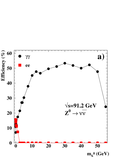
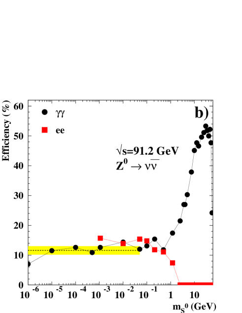
Figure 10: The efficiency versus the $\mathrm{S}^{0}$ mass at $\sqrt{s}=91$ GeV for the decay $\mathrm{S}^{0}\mathrm{Z}^{0}\to\gamma\gamma\nu\overline{\nu}$ and $\mathrm{S}^{0}\mathrm{Z}^{0}\to\mathrm{e}^{+}\mathrm{e}^{-}\nu\overline{\nu}$. a) in linear mass scale and b) in logarithmic mass scale. The dashed line indicates the average of the efficiencies for $m_{\mathrm{S}^{0}}\leq 50~{}\mbox{MeV}$. The shaded bands show the typical error on the efficiencies in this region.

Figure 13: Exclusion limits on the perturbative mass scale $m_{\mathrm{C}}$ for constant $\tilde{K}$. The solid line represents the limits obtained from the data, and the dotted line shows the expected limit if there were only background. Values for $m_{\mathrm{C}}$ below the lines are excluded by this analysis at the 95 % confidence level.

References

- [1] The OPAL Collaboration, P.D. Acton et al., Phys. Lett. B268 (1991) 122.
-
[2]
G.G. Hanson, Proceedings of the XX International Symposium on Lepton
and Photon Interactions at High Energies, Rome, Italy, July 23–28, 2001;
The ALEPH Collaboration, A. Heister et al., Phys. Lett. B526 (2002) 191;
The DELPHI Collaboration, P. Abreu et al., Phys. Lett. B499 (2001) 23;
The L3 Collaboration, P. Achard et al., Phys. Lett. B517 (2001) 319;