EUROPEAN ORGANIZATION FOR NUCLEAR RESEARCH

CERN-EP-2002-031

10 May 2002

Measurement of the Charm
Structure Function $F_{2,\mathrm{c}}^{\gamma}$
of the Photon at LEP

The OPAL Collaboration

Abstract

The production of charm quarks is studied in deep-inelastic electron-photon scattering using data recorded by the OPAL detector at LEP at nominal $\mathrm{e}^{+}\mathrm{e}^{-}$ centre-of-mass energies from 183 to 209 GeV. The charm quarks have been identified by full reconstruction of charged ${\mathrm{D}^{\star}}$ mesons using their decays into ${\mathrm{D}^{0}}\pi$ with the ${\mathrm{D}^{0}}$ observed in two decay modes with charged particle final states, ${\rm K}\pi$ and ${\rm K}\pi\pi\pi$. The cross-section $\sigma^{{\mathrm{D}^{\star}}}$ for production of charged ${\mathrm{D}^{\star}}$ in the reaction $\mathrm{e}^{+}\mathrm{e}^{-}\to\mathrm{e}^{+}\mathrm{e}^{-}\,{\mathrm{D}^{\star}}\,X$ is measured in a restricted kinematical region using two bins in Bjorken $x$, $0.0014<x<0.1$ and $0.1<x<0.87$. From $\sigma^{{\mathrm{D}^{\star}}}$ the charm production cross-section $\sigma(\mathrm{e}^{+}\mathrm{e}^{-}\to\mathrm{e}^{+}\mathrm{e}^{-}\,\mathrm{c\bar{c}}\,X)$ and the charm structure function of the photon $F_{2,\mathrm{c}}^{\gamma}$ are determined in the region $0.0014<x<0.87$ and $5<Q^{2}<100$ $\mathrm{GeV}^{2}$. For $x>0.1$ the perturbative QCD calculation at next-to-leading order agrees perfectly with the measured cross-section. For $x<0.1$ the measured cross-section is $43.8\pm 14.3\pm 6.3\pm 2.8$ $\mathrm{pb}$ with a next-to-leading order prediction of $17.0\,^{+\,2.9}_{-\,2.3}$ $\mathrm{pb}$.

(Submitted to Physics Letters B)

G. Abbiendi², C. Ainsley⁵, P.F. Åkesson³, G. Alexander²², J. Allison¹⁶, P. Amaral⁹, G. Anagnostou¹, K.J. Anderson⁹, S. Arcelli², S. Asai²³, D. Axen²⁷, G. Azuelos^18,a, I. Bailey²⁶, E. Barberio⁸, R.J. Barlow¹⁶, R.J. Batley⁵, P. Bechtle²⁵, T. Behnke²⁵, K.W. Bell²⁰, P.J. Bell¹, G. Bella²², A. Bellerive⁶, G. Benelli⁴, S. Bethke³², O. Biebel³², I.J. Bloodworth¹, O. Boeriu¹⁰, P. Bock¹¹, D. Bonacorsi², M. Boutemeur³¹, S. Braibant⁸, L. Brigliadori², R.M. Brown²⁰, K. Buesser²⁵, H.J. Burckhart⁸, J. Cammin³, S. Campana⁴, R.K. Carnegie⁶, B. Caron²⁸, A.A. Carter¹³, J.R. Carter⁵, C.Y. Chang¹⁷, D.G. Charlton^1,b, I. Cohen²², A. Csilling^8,g, M. Cuffiani², S. Dado²¹, G.M. Dallavalle², S. Dallison¹⁶, A. De Roeck⁸, E.A. De Wolf⁸, K. Desch²⁵, M. Donkers⁶, J. Dubbert³¹, E. Duchovni²⁴, G. Duckeck³¹, I.P. Duerdoth¹⁶, E. Elfgren¹⁸, E. Etzion²², F. Fabbri², L. Feld¹⁰, P. Ferrari¹², F. Fiedler³¹, I. Fleck¹⁰, M. Ford⁵, A. Frey⁸, A. Fürtjes⁸, P. Gagnon¹², J.W. Gary⁴, G. Gaycken²⁵, C. Geich-Gimbel³, G. Giacomelli², P. Giacomelli², M. Giunta⁴, J. Goldberg²¹, E. Gross²⁴, J. Grunhaus²², M. Gruwé⁸, P.O. Günther³, A. Gupta⁹, C. Hajdu²⁹, M. Hamann²⁵, G.G. Hanson⁴, K. Harder²⁵, A. Harel²¹, M. Harin-Dirac⁴, M. Hauschild⁸, J. Hauschildt²⁵, R. Hawkings⁸, R.J. Hemingway⁶, C. Hensel²⁵, G. Herten¹⁰, R.D. Heuer²⁵, J.C. Hill⁵, K. Hoffman⁹, R.J. Homer¹, D. Horváth^29,c, R. Howard²⁷, P. Hüntemeyer²⁵, P. Igo-Kemenes¹¹, K. Ishii²³, H. Jeremie¹⁸, P. Jovanovic¹, T.R. Junk⁶, N. Kanaya²⁶, J. Kanzaki²³, G. Karapetian¹⁸, D. Karlen⁶, V. Kartvelishvili¹⁶, K. Kawagoe²³, T. Kawamoto²³, R.K. Keeler²⁶, R.G. Kellogg¹⁷, B.W. Kennedy²⁰, D.H. Kim¹⁹, K. Klein¹¹, A. Klier²⁴, S. Kluth³², T. Kobayashi²³, M. Kobel³, T.P. Kokott³, S. Komamiya²³, L. Kormos²⁶, R.V. Kowalewski²⁶, T. Krämer²⁵, T. Kress⁴, P. Krieger^6,l, J. von Krogh¹¹, D. Krop¹², M. Kupper²⁴, P. Kyberd¹³, G.D. Lafferty¹⁶, H. Landsman²¹, D. Lanske¹⁴, J.G. Layter⁴, A. Leins³¹, D. Lellouch²⁴, J. Letts¹², L. Levinson²⁴, J. Lillich¹⁰, S.L. Lloyd¹³, F.K. Loebinger¹⁶, J. Lu²⁷, J. Ludwig¹⁰, A. Macpherson^28,i, W. Mader³, S. Marcellini², T.E. Marchant¹⁶, A.J. Martin¹³, J.P. Martin¹⁸, G. Masetti², T. Mashimo²³, P. Mättig^m, W.J. McDonald²⁸, J. McKenna²⁷, T.J. McMahon¹, R.A. McPherson²⁶, F. Meijers⁸, P. Mendez-Lorenzo³¹, W. Menges²⁵, F.S. Merritt⁹, H. Mes^6,a, A. Michelini², S. Mihara²³, G. Mikenberg²⁴, D.J. Miller¹⁵, S. Moed²¹, W. Mohr¹⁰, T. Mori²³, A. Mutter¹⁰, K. Nagai¹³, I. Nakamura²³, H.A. Neal³³, R. Nisius⁸, S.W. O’Neale¹, A. Oh⁸, A. Okpara¹¹, M.J. Oreglia⁹, S. Orito²³, C. Pahl³², G. Pásztor^8,g, J.R. Pater¹⁶, G.N. Patrick²⁰, J.E. Pilcher⁹, J. Pinfold²⁸, D.E. Plane⁸, B. Poli², J. Polok⁸, O. Pooth¹⁴, M. Przybycień^8,j, A. Quadt³, K. Rabbertz⁸, C. Rembser⁸, P. Renkel²⁴, H. Rick⁴, J.M. Roney²⁶, S. Rosati³, Y. Rozen²¹, K. Runge¹⁰, D.R. Rust¹², K. Sachs⁶, T. Saeki²³, O. Sahr³¹, E.K.G. Sarkisyan^8,j, A.D. Schaile³¹, O. Schaile³¹, P. Scharff-Hansen⁸, J. Schieck³², T. Schoerner-Sadenius⁸, M. Schröder⁸, M. Schumacher³, C. Schwick⁸, W.G. Scott²⁰, R. Seuster^14,f, T.G. Shears^8,h, B.C. Shen⁴, C.H. Shepherd-Themistocleous⁵, P. Sherwood¹⁵, G. Siroli², A. Skuja¹⁷, A.M. Smith⁸, R. Sobie²⁶, S. Söldner-Rembold^10,d, S. Spagnolo²⁰, F. Spano⁹, A. Stahl³, K. Stephens¹⁶, D. Strom¹⁹, R. Ströhmer³¹, S. Tarem²¹, M. Tasevsky⁸, R.J. Taylor¹⁵, R. Teuscher⁹, M.A. Thomson⁵, E. Torrence¹⁹, D. Toya²³, P. Tran⁴, T. Trefzger³¹, A. Tricoli², I. Trigger⁸, Z. Trócsányi^30,e, E. Tsur²², M.F. Turner-Watson¹, I. Ueda²³, B. Ujvári^30,e, B. Vachon²⁶, C.F. Vollmer³¹, P. Vannerem¹⁰, M. Verzocchi¹⁷, H. Voss⁸, J. Vossebeld⁸, D. Waller⁶, C.P. Ward⁵, D.R. Ward⁵, P.M. Watkins¹, N.K. Watson¹, P.S. Wells⁸, T. Wengler⁸, N. Wermes³, D. Wetterling¹¹ G.W. Wilson^16,k, J.A. Wilson¹, G. Wolf²⁴, T.R. Wyatt¹⁶, S. Yamashita²³, V. Zacek¹⁸, D. Zer-Zion⁴, L. Zivkovic²⁴

¹School of Physics and Astronomy, University of Birmingham, Birmingham B15 2TT, UK
²Dipartimento di Fisica dell’ Università di Bologna and INFN, I-40126 Bologna, Italy
³Physikalisches Institut, Universität Bonn, D-53115 Bonn, Germany
⁴Department of Physics, University of California, Riverside CA 92521, USA
⁵Cavendish Laboratory, Cambridge CB3 0HE, UK
⁶Ottawa-Carleton Institute for Physics, Department of Physics, Carleton University, Ottawa, Ontario K1S 5B6, Canada
⁸CERN, European Organisation for Nuclear Research, CH-1211 Geneva 23, Switzerland
⁹Enrico Fermi Institute and Department of Physics, University of Chicago, Chicago IL 60637, USA
¹⁰Fakultät für Physik, Albert-Ludwigs-Universität Freiburg, D-79104 Freiburg, Germany
¹¹Physikalisches Institut, Universität Heidelberg, D-69120 Heidelberg, Germany
¹²Indiana University, Department of Physics, Swain Hall West 117, Bloomington IN 47405, USA
¹³Queen Mary and Westfield College, University of London, London E1 4NS, UK
¹⁴Technische Hochschule Aachen, III Physikalisches Institut, Sommerfeldstrasse 26-28, D-52056 Aachen, Germany
¹⁵University College London, London WC1E 6BT, UK
¹⁶Department of Physics, Schuster Laboratory, The University, Manchester M13 9PL, UK
¹⁷Department of Physics, University of Maryland, College Park, MD 20742, USA
¹⁸Laboratoire de Physique Nucléaire, Université de Montréal, Montréal, Quebec H3C 3J7, Canada
¹⁹University of Oregon, Department of Physics, Eugene OR 97403, USA
²⁰CLRC Rutherford Appleton Laboratory, Chilton, Didcot, Oxfordshire OX11 0QX, UK
²¹Department of Physics, Technion-Israel Institute of Technology, Haifa 32000, Israel
²²Department of Physics and Astronomy, Tel Aviv University, Tel Aviv 69978, Israel
²³International Centre for Elementary Particle Physics and Department of Physics, University of Tokyo, Tokyo 113-0033, and Kobe University, Kobe 657-8501, Japan
²⁴Particle Physics Department, Weizmann Institute of Science, Rehovot 76100, Israel
²⁵Universität Hamburg/DESY, II Institut für Experimental Physik, Notkestrasse 85, D-22607 Hamburg, Germany
²⁶University of Victoria, Department of Physics, P O Box 3055, Victoria BC V8W 3P6, Canada
²⁷University of British Columbia, Department of Physics, Vancouver BC V6T 1Z1, Canada
²⁸University of Alberta, Department of Physics, Edmonton AB T6G 2J1, Canada
²⁹Research Institute for Particle and Nuclear Physics, H-1525 Budapest, P O Box 49, Hungary
³⁰Institute of Nuclear Research, H-4001 Debrecen, P O Box 51, Hungary
³¹Ludwig-Maximilians-Universität München, Sektion Physik, Am Coulombwall 1, D-85748 Garching, Germany
³²Max-Planck-Institut für Physik, Föhringer Ring 6, D-80805 München, Germany
³³Yale University, Department of Physics, New Haven, CT 06520, USA

^a and at TRIUMF, Vancouver, Canada V6T 2A3
^b and Royal Society University Research Fellow
^c and Institute of Nuclear Research, Debrecen, Hungary
^d and Heisenberg Fellow
^e and Department of Experimental Physics, Lajos Kossuth University, Debrecen, Hungary
^f and MPI München
^g and Research Institute for Particle and Nuclear Physics, Budapest, Hungary
^h now at University of Liverpool, Dept of Physics, Liverpool L69 3BX, UK
ⁱ and CERN, EP Div, 1211 Geneva 23
^j and Universitaire Instelling Antwerpen, Physics Department, B-2610 Antwerpen, Belgium
^k now at University of Kansas, Dept of Physics and Astronomy, Lawrence, KS 66045, USA
^l now at University of Toronto, Dept of Physics, Toronto, Canada
^m current address Bergische Universität, Wuppertal, Germany

1 Introduction

Much of the present knowledge of the structure of the photon has been obtained from deep-inelastic electron-photon scattering at $\mathrm{e}^{+}\mathrm{e}^{-}$ colliders [1]. With the high statistics available at LEP2, it is possible to investigate the flavour composition of the hadronic structure function $F_{2}^{\gamma}$. The easiest flavour component of $F_{2}^{\gamma}$ to measure directly is the charm part $F_{2,\mathrm{c}}^{\gamma}$, because charmed hadrons like the ${\mathrm{D}^{\star}}$ meson are produced with a large cross-section and can be identified by the well established method of full reconstruction of decays of charged ${\mathrm{D}^{\star}}$ mesons.

The measurement is based on deep-inelastic electron-photon scattering, ${\rm e}(k)\,\gamma(p)\rightarrow{\rm e}(k^{\prime})\,\mathrm{c\bar{c}}\,X$, proceeding via the exchange of a virtual photon, $\gamma^{*}(q)$, (the symbols in brackets denote the four-momentum vectors of the particles). Experimentally, for these events one electron is observed in the detector together with a hadronic final state, and the second electron, which is only slightly deflected, leaves the detector unobserved. The determination of $F_{2,\mathrm{c}}^{\gamma}$ exploits the fact that the differential cross-section of this reaction as function of $Q^{2}=-q^{2}$ and Bjorken $x$, defined as $x={Q^{2}}/{(2p\cdot q)}$, is proportional to $F_{2,\mathrm{c}}^{\gamma}(x,Q^{2})$.

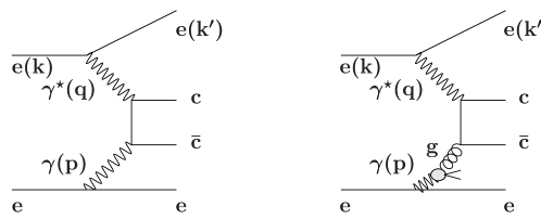
Figure 1: Examples of leading order diagrams contributing to a) the point-like, and b) the hadron-like part of $F_{2,\mathrm{c}}^{\gamma}$.

For a given gluon distribution function, the contribution to $F_{2}^{\gamma}$ from charm quarks can be calculated in perturbative QCD, thanks to the sufficiently large scale established by the charm mass, and predictions have been evaluated at next-to-leading order (NLO) accuracy in [2]. As for light quarks, $F_{2,\mathrm{c}}^{\gamma}$ receives contributions from the point-like and the hadron-like components of the photon structure, as shown schematically in Figure 1. These two contributions are predicted to have different dependences on $x$, with the hadron-like component dominating at very low values of $x$ and the point-like part accounting for most of $F_{2,\mathrm{c}}^{\gamma}$ at $x>0.1$.

The analysis presented here is an extension of the measurement of $F_{2,\mathrm{c}}^{\gamma}$ presented in [3], using basically the same analysis strategy, but a much larger data sample and refined Monte Carlo models. It is based on data recorded by the OPAL experiment in the years 1997–2000, with an integrated luminosity of ${\cal L}=654.1$ $\mathrm{pb}^{-1}$ for nominal $\mathrm{e}^{+}\mathrm{e}^{-}$ centre-of-mass energies, $\sqrt{s_{\rm ee}}$, from 183 to 209 GeV, with a luminosity weighted average of $\sqrt{s_{\rm ee}}=196.6$ GeV.

2 The OPAL detector

A detailed description of the OPAL detector can be found in [4], and therefore only a brief account of the main features relevant to the present analysis is given here.

The central tracking system is located inside a solenoidal magnet which provides a uniform axial magnetic field of 0.435 T along the beam axis. The magnet is surrounded by a lead-glass electromagnetic calorimeter (ECAL) and a hadronic sampling calorimeter (HCAL). Outside the HCAL, the detector is surrounded by muon chambers. There are similar layers of detectors in the endcaps. The region around the beam pipe on both sides of the detector is covered by the forward calorimeters and the silicon-tungsten luminometers.

Starting with the innermost components, the tracking system consists of a high precision silicon microvertex detector [5], a precision vertex drift chamber, a large volume jet chamber with 159 layers of axial anode wires, and a set of $z$ chambers measuring the track coordinates along the beam direction. The transverse momenta $p_{\mathrm{t}}$ of tracks with respect to the $z$ direction of the detector are measured with a precision of $\sigma_{p_{\mathrm{t}}}/p_{\mathrm{t}}=\sqrt{0.02^{2}+(0.0015\cdot p_{\mathrm{t}})^{2}}$ ($p_{\mathrm{t}}$ in GeV) in the central region, where $|\cos\theta|<0.73$. The jet chamber also provides energy loss, ${\mathrm{d}}E/{\mathrm{d}}x$, measurements which are used for particle identification.

The ECAL covers the complete azimuthal range for polar angles satisfying $|\cos\theta|<0.98$. The barrel section, which covers the polar angle range $|\cos\theta|<0.82$, consists of a cylindrical array of 9440 lead-glass blocks with a depth of $24.6$ radiation lengths. The endcap sections (EE) consist of 1132 lead-glass blocks at each end with a depth of more than $22$ radiation lengths, covering the polar angle region of $0.82<|\cos\theta|<0.98$.

The forward calorimeters (FD) at each end of the OPAL detector consist of cylindrical lead-scintillator calorimeters with a depth of 24 radiation lengths divided azimuthally into 16 segments. The electromagnetic energy resolution is about $18\%/\sqrt{E}$ ($E$ in GeV). The acceptance of the forward calorimeters covers the angular range between 47 and 140 mrad from the beam direction. Three planes of proportional tube chambers at 4 radiation lengths depth in the calorimeter measure the direction of electron showers with a precision of approximately 1 mrad.

The silicon tungsten detectors (SW) [6] are located in front of the forward calorimeters at each end of the OPAL detector. Their clear acceptance covers a polar angular region between 33 and 59 mrad. Each calorimeter consists of 19 layers of silicon detectors and 18 layers of tungsten, corresponding to a total of 22 radiation lengths. Each silicon layer consists of 16 wedge-shaped silicon detectors. The electromagnetic energy resolution is about $25\%/\sqrt{E}$ ($E$ in GeV). The radial position of electron showers in the SW calorimeter can be determined with a typical resolution of 0.06 mrad in the polar angle $\theta$. The SW detector provides the luminosity measurement.

3 Monte Carlo simulation

The Monte Carlo models HERWIG6.1 [7] and PYTHIA6.1 [8], both based on leading order (LO) matrix elements and parton showers, are used to model the deep-inelastic electron-photon scattering events $\mathrm{e}^{+}\mathrm{e}^{-}\to\mathrm{e}^{+}\mathrm{e}^{-}\mathrm{c\bar{c}}\,X$. For both Monte Carlo models, the charm quark mass is chosen to be $m_{\mathrm{c}}=1.5$ GeV.

In HERWIG6.1, the cross-section is evaluated separately for the point-like and hadron-like contributions using matrix elements for massive quarks, together with the GRV parametrisation [9] for the gluon distribution of the photon. This is an improvement compared to the analysis presented in [3], where HERWIG5.9 was used with matrix elements for massless quarks only. For that model the effect of the charm quark mass was accounted for only rather crudely by not simulating events with hadronic masses of less than $2m_{\rm c}$. The fragmentation into hadrons is based on the cluster model for HERWIG6.1, using the OPAL tune.

To obtain an estimate of the dependence of the measurements on the details of the modelling of ${\mathrm{D}^{\star}}$ production and fragmentation, a second model, based on the PYTHIA program, is used. The spectrum of photons with varying virtualities is generated in PYTHIA [10]. The point-like and the hadron-like processes, which in PYTHIA are denoted by direct and resolved, are then simulated separately using the matrix elements for the production of massive charm quarks, $\gamma\gamma\to\mathrm{c\bar{c}}$ (subprocess ISUB=85) and $\gamma{\rm g}\to\mathrm{c\bar{c}}$ (subprocess ISUB=84). Since these matrix elements are valid only for real photons ($Q^{2}=0$) the $Q^{2}$ dependence of the cross-sections is not expected to be correctly modelled. The cross-sections for both contributions are therefore taken from HERWIG, and PYTHIA is only used for shape comparisons. In PYTHIA the fragmentation into hadrons is simulated using the Lund string model.

All Monte Carlo events were passed through the full simulation of the OPAL detector [11]. They are analysed using the same reconstruction algorithms as applied to the data.

4 Kinematics and data selection

To measure $F_{2,\mathrm{c}}^{\gamma}(x,Q^{2})$, the distribution of events in $x$ and $Q^{2}$ is needed. These variables are related to the experimentally measurable quantities $E_{\mathrm{tag}}$ and $\theta_{\rm tag}$ by:

$$Q^{2}=2\,E_{\mathrm{b}}\,E_{\mathrm{tag}}\,(1-\cos\theta_{\rm tag})$$ (1)

and

$$x=\frac{Q^{2}}{Q^{2}+W^{2}+P^{2}}\,,$$ (2)

where $E_{\mathrm{b}}$ is the energy of the beam electrons, $E_{\mathrm{tag}}$ and $\theta_{\rm tag}$ are the energy and polar angle of the deeply inelastically scattered electron, $W^{2}$ is the invariant mass squared of the hadronic final state, and $P^{2}=-p^{2}$ is the negative value of the virtuality squared of the quasi-real photon. It is required that the associated electron is not seen in the detector. This ensures that $P^{2}\ll Q^{2}+W^{2}$, therefore $P^{2}$ is neglected when calculating $x$ from Equation 2. The electron mass is neglected throughout.

Deep-inelastic electron-photon scattering candidate events are selected as follows:

• The calorimeter cluster with the highest energy in either SW or FD is taken as the electron candidate. The polar angle $\theta_{\rm tag}$ is measured with respect to the original beam direction. An electron candidate is required to have $E_{\mathrm{tag}}>0.5E_{\mathrm{b}}$ and $33<\theta_{\rm tag}<55$ mrad (SW) or $60<\theta_{\rm tag}<120$ mrad (FD).

• To ensure that the virtuality of the quasi-real photon is small, the highest energy electromagnetic cluster in the SW and FD detectors in the hemisphere opposite the scattered electron must have an energy $E_{\mathrm{a}}\leq 0.25\,E_{\mathrm{b}}$ (the anti-tag condition).

• At least three tracks must be found in the tracking chambers. A track is required to have a minimum transverse momentum with respect to the beam axis of 0.12 $\mathrm{GeV}$, and to fulfill standard quality criteria [3].

• To reduce background from $\mathrm{e}^{+}\mathrm{e}^{-}$ annihilation events with charged ${\mathrm{D}^{\star}}$ mesons in the final state, the sum of the energy of all calorimeter clusters in the ECAL is required to be less than 0.5$E_{\mathrm{b}}$. Electromagnetic calorimeter clusters have to pass an energy threshold of 0.1 $\mathrm{GeV}$ for the barrel section and 0.25 $\mathrm{GeV}$ for the endcap sections.

• To reduce the $\mathrm{e}^{+}\mathrm{e}^{-}$ annihilation background further, the visible invariant mass of the event, $W_{\mathrm{vis}}$, should be less than 0.65$E_{\mathrm{b}}$. The invariant mass $W_{\mathrm{vis}}$ is calculated using the momenta of tracks and using the energies and positions of clusters measured in the ECAL, the HCAL, the FD and the SW calorimeters. Clusters in the SW and FD in the hemisphere of the tagged electron are excluded. A matching algorithm [12] is applied to avoid double counting the energy of particles that produce both tracks and clusters. All tracks, except for the kaon candidate identified in the ${\mathrm{D}^{\star}}$ reconstruction, are assumed to be pions.

• A fully reconstructed charged ${\mathrm{D}^{\star}}$ candidate has to be present. The transverse momentum of the ${\mathrm{D}^{\star}}$ with respect to the beam axis, $p_{\mathrm{t}}^{{\mathrm{D}^{\star}}}$, should fulfill $p_{\mathrm{t}}^{{\mathrm{D}^{\star}}}>1(3)$ $\mathrm{GeV}$ for SW(FD)-tagged events, and the pseudorapidity $\eta^{{\mathrm{D}^{\star}}}$ should be in the range $|\eta^{{\mathrm{D}^{\star}}}|<1.5$. The ${\mathrm{D}^{\star}}$ mesons are identified using their decay into ${\mathrm{D}^{0}}\pi$ with the ${\mathrm{D}^{0}}$ observed in two decay modes with charged particle final states, ${\rm K}\pi$ and ${\rm K}\pi\pi\pi$. The following quality criteria are applied to the ${\mathrm{D}^{0}}$ candidate. For the kaon candidate, the ${\mathrm{d}}E/{\mathrm{d}}x$ probability for the kaon hypothesis should exceed 10$\%$, and for all pion candidates the pion probability should be above 0.5$\%$. In addition, the mass of the ${\mathrm{D}^{0}}$ candidate should lie in the window 1.79–1.94 $\mathrm{GeV}$, and the cosine of the angle between the kaon momentum in the ${\mathrm{D}^{0}}$ rest frame and the ${\mathrm{D}^{0}}$ momentum in the laboratory frame should be below 0.9. The cut on the cosine of the angle reduces the background which peaks at 1, whereas the pseudo-scalar ${\mathrm{D}^{0}}$ decays isotropically in its rest frame.

With these cuts 1653 events are selected in the data having $\Delta m<0.21$ $\mathrm{GeV}$, where $\Delta m$ is the difference between the ${\mathrm{D}^{\star}}$ and ${\mathrm{D}^{0}}$ candidate masses. They are shown in Figure 2. The number of events reconstructed in the signal region defined by $0.1424<\Delta m<0.1484$ $\mathrm{GeV}$ is 115. No event with more than one ${\mathrm{D}^{\star}}$ candidate in the signal region has been found in the data.

Using Monte Carlo simulations, the expected background to the deep-inelastic electron-photon scattering events from all other Standard Model physics processes that potentially contain final state ${\mathrm{D}^{\star}}$ mesons is found to be about one event and is neglected. The background from random coincidences between off-momentum beam electrons faking a scattered electron and photon-photon scattering events without an observed electron has been estimated to be below 1.4 events and has been neglected. Thus, only the combinatorial background from deep-inelastic electron-photon scattering events $\mathrm{e}^{+}\mathrm{e}^{-}\to\mathrm{e}^{+}\mathrm{e}^{-}\mathrm{q\bar{q}}$ with ${\rm q}={\rm u},{\rm d},{\rm s}\mbox{ and }{\rm c}$ has to be subtracted from the data. The production of bottom quarks is suppressed compared to charm production due to the larger mass and smaller charge and is negligible [1].

5 Results

5.1 Comparison of data and theoretical predictions

Figure 2 shows the difference between the ${\mathrm{D}^{\star}}$ and ${\mathrm{D}^{0}}$ candidate masses for both decay channels combined. A clear peak is observed around the mass difference between the ${\mathrm{D}^{\star}}$ and the ${\mathrm{D}^{0}}$ meson, which is $\Delta m_{0}=0.1454$ $\mathrm{GeV}$ [13]. The number of signal events, $N_{\rm rec}^{{\mathrm{D}^{\star}}}$, has been obtained from an unbinned maximum likelihood fit to this distribution. Similar fits are performed in two regions of $x_{\mathrm{vis}}$, calculated from Equation 2 using $W_{\mathrm{vis}}$ and the measured value of $Q^{2}$. The fit function contains a Gaussian for the signal and a power law function of the form $a\cdot(\Delta m-m_{\pi})^{b}$, for the background contribution. Because the number of signal events is small, the mean value of the Gaussian is kept fixed to the PDG value in the fit. The width and the normalisation are determined by the fit, which gives $55.3\pm 11.0$ signal events, with $23.6\pm 7.4$ and $31.4\pm 8.1$ events for $x_{\mathrm{vis}}<0.1$ and $x_{\mathrm{vis}}>0.1$, where the uncertainties are statistical. The fitted width is $0.70\pm 0.16$ $\mathrm{MeV}$ when using the whole sample. The quality of the fit is satisfactory. The $\chi^{2}$ between the fitted curve and the data in Figure 2 is 94 for 71 non-empty bins. The corresponding $\chi^{2}$ for events with $x_{\mathrm{vis}}<0.1$ and $x_{\mathrm{vis}}>0.1$ are 71 and 93.

The result of the fit for all events is shown in Figure 2 together with the absolute prediction of the combinatorial background measured from the data using events with a wrong-charge pion for the ${\mathrm{D}^{\star}}\to{\mathrm{D}^{0}}\pi$ decays. The fit agrees with this second estimate of the combinatorial background. The numbers of signal events for $x_{\mathrm{vis}}<0.1$ and $x_{\mathrm{vis}}>0.1$ predicted by the HERWIG model are $12.1\pm 0.6$ and $30.0\pm 1.1$, where the uncertainties are statistical.

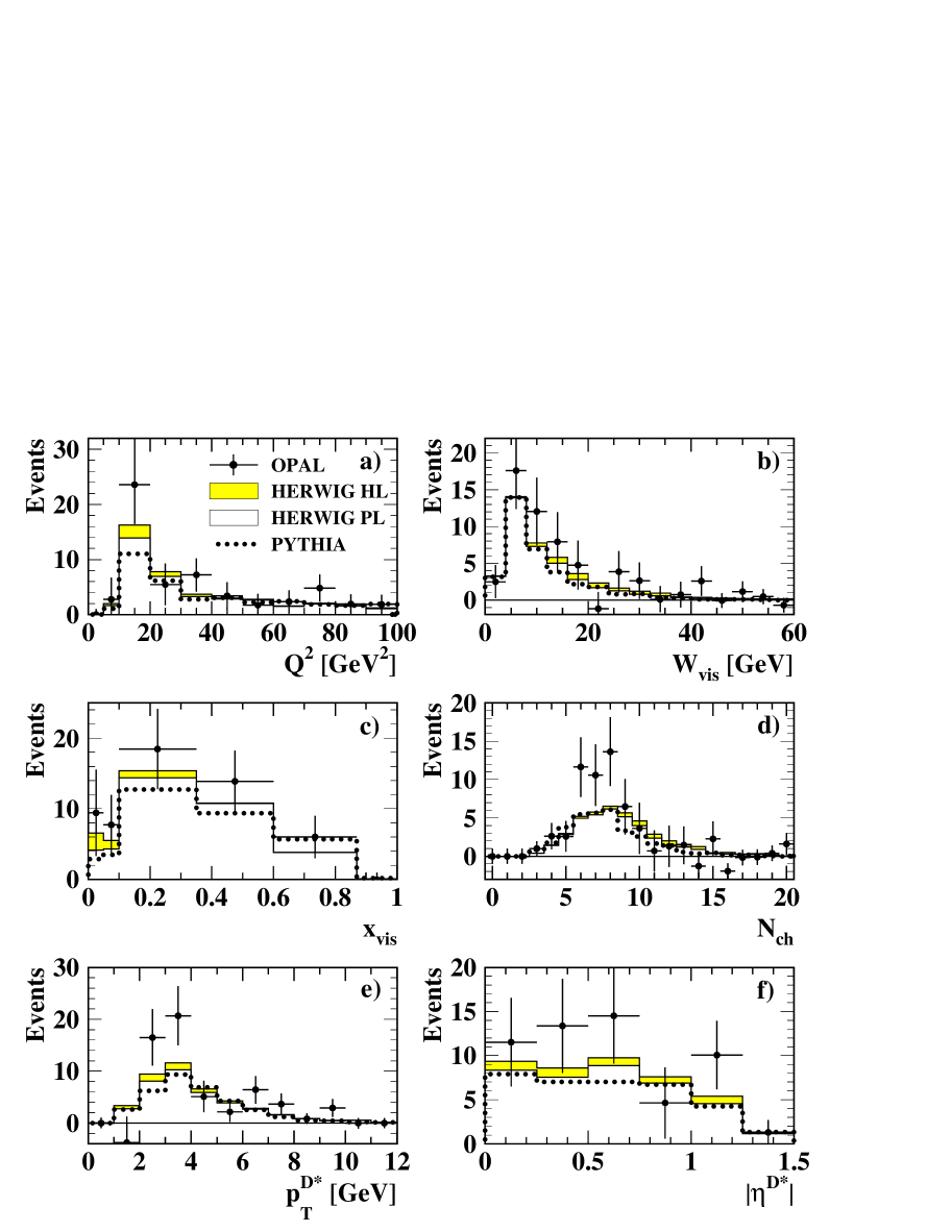
Figure 3: Background subtracted data distributions compared to predictions based on the HERWIG and PYTHIA programs. For HERWIG the hadron-like component is shown as a shaded histogram on top of the open histogram representing the point-like component. The Monte Carlo predictions are normalised to the data luminosity. Shown are a) $Q^{2}$, b) the visible invariant mass, $W_{\mathrm{vis}}$, c) $x_{\mathrm{vis}}$, d) the charged multiplicity, $N_{\mathrm{ch}}$, e) the transverse momentum of the ${\mathrm{D}^{\star}}$ with respect to the beam axis, $p_{\mathrm{t}}^{{\mathrm{D}^{\star}}}$, and f) the absolute value of the pseudorapidity $|\eta^{{\mathrm{D}^{\star}}}|$. The data are shown by points with error bars representing the statistical error.

Figure 3 shows, for the signal events, the distributions of four global event quantities, $Q^{2}$, $W_{\mathrm{vis}}$, $x_{\mathrm{vis}}$ and the charged multiplicity $N_{\mathrm{ch}}$, and two variables related to the kinematics of the ${\mathrm{D}^{\star}}$ candidates, $p_{\mathrm{t}}^{{\mathrm{D}^{\star}}}$ and $|\eta^{{\mathrm{D}^{\star}}}|$. The signal events are shown for the $\Delta m$ region $0.1424<\Delta m<0.1484$ $\mathrm{GeV}$, after subtracting the combinatorial background in that region. The normalisation of the background is given by the result of the fit for the complete sample. The shape of the background distributions is taken from the data using both the events with the wrong-charge combinations and the events with the correct charge combinations that fulfill $0.16<\Delta m<0.21$ $\mathrm{GeV}$, see Figure 2. It has been verified from Monte Carlo that in this range the distributions shown are independent of $\Delta m$. Subtracting the background this way is statistically more precise than using only the events with the wrong-charge combinations in the signal region. The data are compared to the prediction of the HERWIG and PYTHIA Monte Carlo models, normalised to the data luminosity. For the HERWIG prediction the hadron-like component (HERWIG HL) is shown on top of the point-like component (HERWIG PL). Overall, the HERWIG model describes the data distributions quite well, and the shape of the PYTHIA prediction is also consistent with the data.

In what follows, the cross-sections has been calculated based on the HERWIG prediction, while the PYTHIA program was used as a second Monte Carlo model to estimate the uncertainty stemming from the Monte Carlo description of the data.

5.2 Determination of the charm production cross-section

The inclusive cross-section $\sigma^{{\mathrm{D}^{\star}}}$ has been extracted in a well-measured kinematic region where $p_{\mathrm{t}}^{{\mathrm{D}^{\star}}}>1$ $\mathrm{GeV}$ for an electron scattering angle of $33-55$ mrad, or $p_{\mathrm{t}}^{{\mathrm{D}^{\star}}}>3$ $\mathrm{GeV}$ for $60-120$ mrad, $|\eta^{{\mathrm{D}^{\star}}}|<1.5$ and $5<Q^{2}<100$ $\mathrm{GeV}^{2}$, using almost the whole accessible $Q^{2}$ range defined by $\theta_{\rm tag}$ and $E_{\mathrm{tag}}$.

As in the previous investigation [3], the analysis is performed in two bins in $x$, $0.0014<x<0.1$ and $0.1<x<0.87$. The $x$ range is limited by the $Q^{2}$ range, by the minimum kinematically allowed invariant mass $W=3.88$ $\mathrm{GeV}$ needed for the production of a ${\mathrm{D}^{\star}}$ meson together with a second charmed hadron, and by the event selection cut on $W_{\mathrm{vis}}$. To take into account the detector acceptance and resolution in $x$ the data are corrected using a $2\times 2$ matrix, which contains the information of the correlation between the measured value $x_{\mathrm{vis}}$ and the generated $x$ for the two bins in $x$ as given by Monte Carlo. The effects due to the migration in $Q^{2}$ are small compared to those in $x$, and are neglected.

For a given ${\mathrm{D}^{\star}}$ decay channel the selection efficiency for $x<0.1$ is given by the ratio of the number of reconstructed ${\mathrm{D}^{\star}}$ mesons originating from events with $x<0.1$ to all generated ${\mathrm{D}^{\star}}$ mesons in that channel with $x<0.1$ in the restricted kinematic region defined above. For HERWIG6.1, the selection efficiencies for $x<0.1$ are $(16\pm 1)\%$ and $(12\pm 1)\%$ for the point-like and hadron-like components. For $x>0.1$ they are $(19\pm 1)\%$ and $(19\pm 5)\%$ respectively. Combining the two components yields efficiencies of $(15\pm 1)\%$ and $(19\pm 1)\%$ for $x<0.1$ and $x>0.1$. The corresponding selection efficiencies for the PYTHIA sample are $(14\pm 1)\%$ and $(20\pm 1)\%$. This means that in each bin the predicted efficiencies from the HERWIG and PYTHIA models are consistent, so the size of their error of about 10$\%$ is taken as the systematic uncertainty on the efficiency.

Table 1a) summarises the measured values of $\sigma^{{\mathrm{D}^{\star}}}$ for ${\mathrm{D}^{\star}}$ production in the restricted kinematic region defined above:

$$\sigma^{{\mathrm{D}^{\star}}}=\frac{N_{\rm cor}^{{\mathrm{D}^{\star}}}}{{\rm BR}\cdot{\cal L}}.$$ (3)

It is calculated from the number of ${\mathrm{D}^{\star}}$ events, $N_{\rm cor}^{{\mathrm{D}^{\star}}}$, obtained from $N_{\rm rec}^{{\mathrm{D}^{\star}}}$ determined by the likelihood fit to the full sample, together with the $2\times 2$ matrix correction based on the HERWIG model. The statistical correlation between the two data points is $-28\%$. For the combined ${\mathrm{D}^{\star}}$ branching ratios for the 3-prong and 5-prong decay modes, ${\rm BR}=7.66\pm 0.22\,\%$ [13] is used.

The present measurement makes use of the estimation of the systematic error in [3] with some small changes. The statistical error from the background subtraction is treated differently and is now included in the statistical error of the number of signal events determined by the fit. For each of the $x$ regions, a total correlated systematic uncertainty of 10$\%$, as evaluated in [3], is attributed to the sum of the uncertainties stemming from the branching ratios, the imperfectness of the modelling of the central tracking detectors, the kaon identification and the variation of the energy scale of the electron candidate.

For the determination of the cross-section of charm production, $\sigma(\mathrm{e}^{+}\mathrm{e}^{-}\to\mathrm{e}^{+}\mathrm{e}^{-}\,\mathrm{c\bar{c}}\,X)$, the Monte Carlo models are used for extrapolation. This allows $\sigma(\mathrm{e}^{+}\mathrm{e}^{-}\to\mathrm{e}^{+}\mathrm{e}^{-}\,\mathrm{c\bar{c}}\,X)$ to be calculated via the relation

$$\sigma(\mathrm{e}^{+}\mathrm{e}^{-}\to\mathrm{e}^{+}\mathrm{e}^{-}\,\mathrm{c\bar{c}}\,X) = \frac{1}{2\cdot f({\mathrm{c}}\to{\mathrm{D}^{\star}})}\cdot\sigma(\mathrm{e}^{+}\mathrm{e}^{-}\to\mathrm{e}^{+}\mathrm{e}^{-}\,{\mathrm{D}^{\star}}\,X)$$ (4)

$$= \frac{1}{2\cdot f({\mathrm{c}}\to{\mathrm{D}^{\star}})}\cdot{\cal R}^{\mathrm{MC}}\cdot\sigma^{{\mathrm{D}^{\star}}}.$$

The value used for the charm to ${\mathrm{D}^{\star}}$ hadronisation fraction, $f({\mathrm{c}}\to{\mathrm{D}^{\star}})$, is taken to be $0.235\pm 0.007\pm 0.007$, independent of $x$. It has been estimated in [14] by averaging results obtained in $\mathrm{e}^{+}\mathrm{e}^{-}$ annihilation at LEP1 as well as at lower $\mathrm{e}^{+}\mathrm{e}^{-}$ centre-of-mass energies. The extrapolation factor ${\cal R}^{\mathrm{MC}}$ is defined as the ratio of the number of all generated ${\mathrm{D}^{\star}}$ mesons in the full kinematic region of $p_{\mathrm{t}}^{{\mathrm{D}^{\star}}}$ and $|\eta^{{\mathrm{D}^{\star}}}|$ divided by the number of generated ${\mathrm{D}^{\star}}$ mesons in the restricted region. For $x<0.1$ the ${\cal R}^{\mathrm{MC}}$ values for the HERWIG and PYTHIA models are $6.15\pm 0.03$ and $6.23\pm 0.03$, while for $x>0.1$ the corresponding numbers are $4.73\pm 0.02$ and $4.59\pm 0.02$, where the errors are statistical. The central values of the extrapolated cross-sections are obtained using the HERWIG numbers, and the differences between the HERWIG and PYTHIA predictions have been taken as estimates of the extrapolation errors.

In Figure 4a) and Table 1b), the measured cross-sections $\sigma(\mathrm{e}^{+}\mathrm{e}^{-}\to\mathrm{e}^{+}\mathrm{e}^{-}\,\mathrm{c\bar{c}}\,X)$ are compared to the calculation of [2] performed in LO and NLO and to the prediction from HERWIG. The NLO prediction uses $m_{\mathrm{c}}=1.5$ $\mathrm{GeV}$. The renormalisation and factorisation scales are chosen to be $\mu^{2}_{\rm r}=\mu^{2}_{\rm f}=Q^{2}$. The calculation is obtained for the sum of the point-like and hadron-like contributions to $F_{2,\mathrm{c}}^{\gamma}$, where for the calculation of the hadron-like part the GRV-NLO parametrisation is used. These GRV-NLO parton distributions of the photon have been found to describe the OPAL jet data [15]. The NLO corrections are predicted to be small for the whole $x$ range. The NLO calculation is shown in Figure 4 as a band representing the uncertainty of the theoretical prediction, evaluated by varying the charm quark mass between 1.3 and 1.7 GeV and by changing the renormalisation and factorisation scales in the range $Q^{2}/4\leq\mu^{2}_{\rm r}=\mu^{2}_{\rm f}\leq 4Q^{2}$, taking the largest difference from the central value as the error. The HERWIG prediction falls within the uncertainty band of the NLO calculation.

For $x>0.1$, the predicted NLO cross-section in Figure 4a) agrees well with the data. For $x<0.1$, the situation is different. The NLO calculation predicts the hadron-like and point-like component to be of about equal size, and the sum is smaller than what is observed for the data.

The point-like contribution can be calculated with small uncertainties, i.e. in LO it depends only on $m_{\mathrm{c}}$. The prediction for the hadron-like part is more uncertain, especially because it depends on the gluon distribution of the photon, for which experimental information is limited. Given the good agreement at large $x$ between the data and the NLO prediction, dominated by the point-like component, the NLO point-like prediction has been subtracted from the measured cross-section in the region $0.0014<x<0.1$. This leads to the value of $34.5\pm 14.3\pm 6.9$ $\mathrm{pb}$ for the hadron-like contribution to the cross-section, which is to be compared with the NLO prediction of $7.7\,^{+\,2.2}_{-\,1.6}$ $\mathrm{pb}$, when using the GRV-NLO parton distributions of the photon.

5.3 Extraction of $F_{2,\mathrm{c}}^{\gamma}$

The value of the charm structure function $F_{2,\mathrm{c}}^{\gamma}(x,Q^{2})/\alpha$ of the photon, averaged over the corresponding bin in $x$, and given at a fixed value of $Q^{2}$, is determined by

$$F_{2,\mathrm{c}}^{\gamma}(x,Q^{2})/\alpha=\sigma(\mathrm{e}^{+}\mathrm{e}^{-}\to\mathrm{e}^{+}\mathrm{e}^{-}\,\mathrm{c\bar{c}}\,X)\cdot\left(\frac{F_{2,\mathrm{c}}^{\gamma}(x,Q^{2})/\alpha}{\sigma(\mathrm{e}^{+}\mathrm{e}^{-}\to\mathrm{e}^{+}\mathrm{e}^{-}\,\mathrm{c\bar{c}}\,X)}\right)_{\rm NLO},$$ (5)

where the ratio $(F_{2,\mathrm{c}}^{\gamma}(x,Q^{2})/\alpha/\sigma(\mathrm{e}^{+}\mathrm{e}^{-}\to\mathrm{e}^{+}\mathrm{e}^{-}\,\mathrm{c\bar{c}}\,X))_{\rm NLO}$ is given by the NLO calculation of [2]. This approach assumes that for a bin of $x$ the ratio of the structure function, averaged over $x$ and evaluated at the average $Q^{2}$ value of the data, and the cross-section within the region of $Q^{2}$, are the same for the data and the NLO calculation. The measurement is given at $Q^{2}=20$ $\mathrm{GeV}^{2}$, which roughly corresponds to the average value of $Q^{2}$ observed for the data. The $F_{2,\mathrm{c}}^{\gamma}(x,Q^{2})/\alpha$ values are listed in Table 1c) and shown in Figure 4b) on a logarithmic scale in $x$.

In addition to the structure function of the full NLO calculation, the predicted hadron-like component is also shown in Figure 4b). This contribution is very small for $x>0.1$ and therefore in this region the NLO calculation is a perturbative prediction which depends only on the charm quark mass and the strong coupling constant. This prediction agrees perfectly with the data.

To illustrate the shape of $F_{2,\mathrm{c}}^{\gamma}$ the data are also compared to the GRS-LO [16] prediction and to the point-like component alone, both shown for $Q^{2}=20$ $\mathrm{GeV}^{2}$. The point-like contribution is small at low $x$. The data span a rather large range in $Q^{2}$, in which the change of the predicted $F_{2,\mathrm{c}}^{\gamma}$ is large. The maximum value of $F_{2,\mathrm{c}}^{\gamma}$ for $x>0.1$ rises by about a factor of five between the lower boundary of $Q^{2}=5$ $\mathrm{GeV}^{2}$ and the higher boundary of $Q^{2}=100$ $\mathrm{GeV}^{2}$. In addition, the mass threshold, $W=2m_{\mathrm{c}}$, introduces a $Q^{2}$ dependent upper limit in $x$ which, in the $Q^{2}$ range studied, varies from $x=0.35$ to $x=0.9$.

To be able to compare the data directly with the curves from the GRS-LO predictions the points are placed at those $x$ positions that correspond to the average predicted $F_{2,\mathrm{c}}^{\gamma}$ within the bin [17]. These $x$ values are calculated both for the full $F_{2,\mathrm{c}}^{\gamma}$ and for the point-like component alone. The data points are located at the mean of the two values and the horizontal error bar indicates their difference. For $x>0.1$ the difference is invisible in Figure 4b).

For $x<0.1$ the hadron-like contribution to $F_{2,\mathrm{c}}^{\gamma}(x,Q^{2})/\alpha$, determined as for the cross-section, amounts to $0.154\pm 0.059\pm 0.029$, to be compared with the NLO prediction of $0.026\,^{+\,0.007}_{-\,0.005}$.

6 Conclusions

The production of charm quarks is studied in deep-inelastic electron-photon scattering using data recorded by the OPAL detector at LEP at nominal $\mathrm{e}^{+}\mathrm{e}^{-}$ centre-of-mass energies from 183 to 209 GeV in the years 1997–2000. The result is based on 654.1 $\mathrm{pb}^{-1}$ of data with a luminosity weighted average centre-of-mass energy of $196.6$ GeV. The measurement is an extension of the result presented in [3], using basically the same analysis strategy, but with improved Monte Carlo models and higher statistics. The two OPAL results are consistent and the new measurement supersedes the result in [3].

The cross-section $\sigma^{{\mathrm{D}^{\star}}}$ for ${\mathrm{D}^{\star}}$ production in the reaction $\mathrm{e}^{+}\mathrm{e}^{-}\to\mathrm{e}^{+}\mathrm{e}^{-}\,{\mathrm{D}^{\star}}\,X$ is measured in the deep-inelastic scattering regime for a restricted region where $p_{\mathrm{t}}^{{\mathrm{D}^{\star}}}>1$ $\mathrm{GeV}$ for an electron scattering angle of $33-55$ mrad, or $p_{\mathrm{t}}^{{\mathrm{D}^{\star}}}>3$ $\mathrm{GeV}$ for $60-120$ mrad, $|\eta^{{\mathrm{D}^{\star}}}|<1.5$ and $5<Q^{2}<100$ $\mathrm{GeV}^{2}$, divided into two bins in $x$, $0.0014<x<0.1$ and $0.1<x<0.87$. Within errors the cross-sections can be described by the HERWIG model. From $\sigma^{{\mathrm{D}^{\star}}}$ the cross-section $\sigma(\mathrm{e}^{+}\mathrm{e}^{-}\to\mathrm{e}^{+}\mathrm{e}^{-}\,\mathrm{c\bar{c}}\,X)$ is obtained by extrapolation in the same bins of $x$ and $Q^{2}$, using Monte Carlo.

The charm structure function $F_{2,\mathrm{c}}^{\gamma}(x,Q^{2})/\alpha$ of the photon is evaluated at $Q^{2}=20$ $\mathrm{GeV}^{2}$ for the same bins of $x$. For $x>0.1$, the perturbative QCD calculation at next-to-leading order agrees perfectly with the measurement. For $x<0.1$ the point-like component, however calculated, lies below the data. Subtracting the NLO point-like prediction, a measured value for the hadron-like part of $0.154\pm 0.059\pm 0.029$ is obtained.

a)	$\sigma^{{\mathrm{D}^{\star}}}$ [pb]
	$0.0014<x<0.1$	$0.1<x<0.87$
OPAL	$3.1\pm 1.0\pm 0.5$	$2.6\pm 0.9\pm 0.3$
HERWIG	1.13 (0.71 + 0.43)	2.05 (2.02 + 0.03)
b)	$\sigma(\mathrm{e}^{+}\mathrm{e}^{-}\to\mathrm{e}^{+}\mathrm{e}^{-}\,\mathrm{c\bar{c}}\,X)$ [pb]
	$0.0014<x<0.1$	$0.1<x<0.87$
OPAL	$43.8\pm 14.3\pm 6.3\pm 2.8$	$26.2\pm 8.8\pm 3.2\pm 1.3$
HERWIG	17.0 (8.5 +38.4)	27.4 (27.1 + 0.4)
LO	16.0 (8.1 +37.9)	26.7 (26.3 + 0.4)
NLO	$17.0\,^{+\,2.9}_{-\,2.3}$ ($9.3\,^{+\,0.8}_{-\,0.6}$ + $7.7\,^{+\,2.2}_{-\,1.6}$)	$30.8\,^{+\,7.1}_{-\,5.7}$ ($30.4\,^{+\,6.9}_{-\,5.5}$ + $0.4\,^{+\,0.2}_{-\,0.1}$)
c)	$F_{2,\mathrm{c}}^{\gamma}(x,Q^{2})/\alpha$
	$0.0014<x<0.1$	$0.1<x<0.87$
OPAL	$0.180\pm 0.059\pm 0.026\pm 0.012$	$0.084\pm 0.028\pm 0.010\pm 0.004$
LO	0.065	0.084
NLO	$0.070\,^{+\,0.011}_{-\,0.008}$ ($0.044\,^{+\,0.004}_{-\,0.003}$ + $0.026\,^{+\,0.007}_{-\,0.005}$)	$0.099\,^{+\,0.023}_{-\,0.019}$ ($0.098\,^{+\,0.023}_{-\,0.019}$ + 0.001)

Table 1: a) The cross-section $\sigma^{{\mathrm{D}^{\star}}}$ in the restricted region, b) the cross-section $\sigma(\mathrm{e}^{+}\mathrm{e}^{-}\to\mathrm{e}^{+}\mathrm{e}^{-}\,\mathrm{c\bar{c}}\,X)$, extrapolated using Monte Carlo, and c) the structure function $F_{2,\mathrm{c}}^{\gamma}$ at $Q^{2}=20$ $\mathrm{GeV}^{2}$. For the measurements the quoted errors are due, respectively, to statistics, systematics and extrapolation. The statistical correlation between the two data points is $-28\%$. The measurements are compared to several theoretical predictions. The HERWIG prediction in a) uses the value of $f({\mathrm{c}}\to{\mathrm{D}^{\star}})$ contained in the program. The numbers in brackets are separate values for the point-like and hadron-like components, respectively. See text for further details.

Figure 2: Distribution of the difference, $\Delta m$, between the ${\mathrm{D}^{\star}}$ and ${\mathrm{D}^{0}}$ candidate masses for both decay channels combined. The data are shown as points with statistical errors. The histogram represents the combinatorial background estimated using events with a wrong-charge pion for the ${\mathrm{D}^{\star}}\to{\mathrm{D}^{0}}\pi$ decays. The curve is the result of the fit to a Gaussian signal plus a power-law background function, as explained in the text.

Figure 4: OPAL results for a) the cross-section $\sigma(\mathrm{e}^{+}\mathrm{e}^{-}\to\mathrm{e}^{+}\mathrm{e}^{-}\,\mathrm{c\bar{c}}\,X)$, with $5<Q^{2}<100$ $\mathrm{GeV}^{2}$ and b) for the charm structure function of the photon divided by the fine structure constant, $F_{2,\mathrm{c}}^{\gamma}(x,Q^{2})/\alpha$, at $Q^{2}=20$ $\mathrm{GeV}^{2}$. The data points are the results obtained with the HERWIG Monte Carlo model. The outer error bar is the total error and the inner error bar the statistical error. The data points in b) are placed at those $x$ values that correspond to the average predicted $F_{2,\mathrm{c}}^{\gamma}$ within a bin. The data are compared to the calculation of [2] performed in LO and NLO. The band for the NLO calculation indicates the theoretical error from uncertainties in the charm quark mass and renormalisation and factorisation scales. In a) the cross-section prediction of the HERWIG Monte Carlo model is also given. b) also shows the prediction of the GRS-LO parametrisation for the structure function at $Q^{2}=20$ $\mathrm{GeV}^{2}$ and its point-like component separately.

References

- [1] R. Nisius, Phys. Rep. 332, 165–317 (2000).
-
[2]
E. Laenen, S. Riemersma, J. Smith, and W.L. van Neerven,
Phys. Rev. D49, 5753–5768 (1994);
E. Laenen and S. Riemersma, Phys. Lett. B376, 169–176 (1996). - [3] OPAL Collaboration, G. Abbiendi et al., Eur. Phys. J. C16, 579–596 (2000).
- [4] OPAL Collaboration, K. Ahmet et al., Nucl. Instr. and Meth. A305, 275–319 (1991).
-
[5]
P.P. Allport et al., Nucl. Instr. and Meth. A324, 34–52 (1993);
P.P. Allport et al., Nucl. Instr. and Meth. A346, 476–495 (1994). - [6] B.E. Anderson et al., IEEE Transactions on Nuclear Science 41, 845–852 (1994).
- [7] G. Corcella et al., JHEP01, 010 (2001).
- [8] T. Sjöstrand et al., Comp. Phys. Comm. 135, 238–259 (2001).
-
[9]
M. Glück, E. Reya, and A. Vogt, Phys. Rev. D45, 3986–3994 (1992);
M. Glück, E. Reya, and A. Vogt, Phys. Rev. D46, 1973–1979 (1992). - [10] C. Friberg and T. Sjöstrand, Eur. Phys. J. C13, 151–174 (2000).
- [11] J. Allison et al., Nucl. Instr. and Meth. A317, 47–74 (1992).
- [12] OPAL Collaboration, G. Alexander et al., Phys. Lett. B377, 181–194 (1996).
- [13] Particle Data Group, D.E. Groom et al., Eur. Phys. J. C15, 1–878 (2000).
- [14] L. Gladilin, Charm hadron production fractions, hep-ex/9912064 (1999).
- [15] OPAL Collaboration, G. Abbiendi et al., Eur. Phys. J. C10, 547–561 (1999),
- [16] M. Glück, E. Reya, and M. Stratmann, Phys. Rev. D51, 3220–3229 (1995).
- [17] G.D. Lafferty and T.R. Wyatt, Nucl. Instr. and Meth. A355, 541–547 (1995).