REVIEW OF EXPERIMENTAL SEARCHES FOR ${\mathrm{B}}_{\mathrm{s}}$ OSCILLATIONS

Abstract

The current status of experimental searches for ${\mathrm{B}}_{\mathrm{s}}$ oscillations is reviewed. The three ALEPH analyses have been improved since Summer 2001, and submitted for publication. The combination of all available analyses is presented and discussed.

1 Introduction

A search for ${\mathrm{B}}_{\mathrm{s}}$ oscillations consists in detecting the time-dependent difference between the proper time distributions of “mixed” and “unmixed” decays,

$${\cal P}(t)_{{\mathrm{B}}_{\mathrm{s}}\to{\overline{{\mathrm{B}}}_{\mathrm{s}}}} = \frac{\Gamma e^{-\Gamma t}}{2}\,[1-\cos(\Delta m_{\mathrm{s}}\,t)]\ ,$$

$${\cal P}(t)_{{\mathrm{B}}_{\mathrm{s}}\to{\mathrm{B}}_{\mathrm{s}}} = \frac{\Gamma e^{-\Gamma t}}{2}\,[1+\cos(\Delta m_{\mathrm{s}}\,t)]\ .$$ (1)

The amplitude of such difference is damped not only by the natural exponential decay, but also by the effect of the experimental resolution in the proper time reconstruction. The proper time is derived from the measured decay length and the reconstructed momentum of the decaying meson. The resolution on the decay length $\sigma_{L}$ is to first order independent of the decay length itself, and is largely determined by the tracking capabilities of the detector. The momentum resolution $\sigma_{p}$ strongly depends on the final state chosen for a given analysis, and is typically proportional to the momentum itself. The proper time resolution can be therefore written as

$$\sigma_{t}=\frac{m}{p}\sigma_{L}\oplus\frac{\sigma_{p}}{p}\,t\ ,$$ (2)

where the decay length resolution contributes a constant term, and the momentum resolution a term proportional to the proper time. Examples of the observable difference between the proper time distributions of mixed and unmixed decays are shown in Fig. 1, for the simple case of monochromatic ${\mathrm{B}}_{\mathrm{s}}$ mesons, fixed Gaussian resolutions on momentum and decay length (${\sigma_{p}}/{p}=0.15$, ${\sigma_{L}}=250\ \mu{\mathrm{m}}$), and for different values of the oscillation frequency.

Figure 1: Effect of proper time resolution on the decay exponential E($t$), and on the difference between the proper time distributions of unmixed and mixed decays, for several values of the oscillation frequency. Only monochromatic ${\mathrm{B}}_{\mathrm{s}}$ mesons are considered, with perfect separation between mixed and unmixed decays; resolutions are taken to be Gaussian.

For low frequency several periods can be observed. As the frequency increases, the effect of the finite proper time resolution becomes more relevant, inducing an overall decrease of observed difference, and a faster damping as a function of time (due to the momentum resolution component). In the example given, for a frequency of $25\ {\mathrm{ps}}^{-1}$ only a small effect corresponding to the first half-period can be seen.

The experimental knowledge of ${\mathrm{B}}_{\mathrm{s}}$ oscillations available today comes mostly from SLD and the LEP experiments. At SLD the lower statistics (less than $4\times 10^{5}$ hadronic ${\mathrm{Z}}$ decays, compared to almost $4\times 10^{6}$ for each LEP experiment) is compensated, especially at high frequency, by the excellent tracking performance provided by the small and precise CCD vertex detector: at SLD in a typical analysis a decay length resolution of $70-80\ \mu{\mathrm{m}}$ is obtained for a core of $60\%$ of the events, with tails of $250-300\ \mu{\mathrm{m}}$, while at LEP the corresponding figures are $200-250\ \mu{\mathrm{m}}$ and $700-1000\ \mu{\mathrm{m}}$.

2 Analysis methods

Analyses based on different final state selections have been developed over the years, which offer different advantages in terms of statistics, signal purity and resolution. The selection criterion chosen also determines the strategy for tagging the flavour of the ${\mathrm{B}}_{\mathrm{s}}$ meson at decay time. The flavour at production time is tagged from the hemisphere opposite to the one containing the selected candidate, as well as from the fragmentation particles belonging to the candidate hemisphere. Finally, the proper time is reconstructed and the oscillation is studied by means of a likelihood fit to the proper time distributions of mixed and unmixed decays.

2.1 Selection methods and flavour tagging at decay time

In fully inclusive selections no decay product of the ${\mathrm{B}}_{\mathrm{s}}$ is explicitly identified, which implies that no straightforward method is available to tag the flavour at decay time. Variables sensitive to the sign of the charge flow between the secondary and the tertiary vertices (${\mathrm{B}}_{\mathrm{s}}\to{\mathrm{D}}_{\mathrm{s}}^{-}$, ${\overline{{\mathrm{B}}}_{\mathrm{s}}}\to{\mathrm{D}}_{\mathrm{s}}^{+}$) can be built to discriminate between ${\mathrm{B}}_{\mathrm{s}}$ and ${\overline{{\mathrm{B}}}_{\mathrm{s}}}$ decays. This method gives the highest statistics (a few $10^{5}$ candidates at LEP, about $10^{4}$ at SLD); the signal fraction is what is given by nature ($\approx 10\%$). The reconstruction of the secondary vertex is completely based on topology, which requires excellent tracking capabilities, to avoid that the track mis-assignment spoils the decay length reconstruction. The method has high performance at SLD; at LEP it has been attempted by DELPHI: the much more difficult experimental environment results in uncertainties on the fitted amplitude (Section 3) raising fast with increasing frequency (Fig. 2a).

Figure 2: (a) The SLD analyses based on fully inclusive and inclusive lepton selections are compared to the corresponding DELPHI and ALEPH analyses. The error on the measured oscillation amplitude is shown as a function of test frequency.
(b) Error on the measured oscillation amplitude for the ALEPH inclusive lepton analysis, compared to the same analysis when average values are used for the momentum and decay length resolutions (see text).

In semi-inclusive selections at least one ${\mathrm{B}}_{\mathrm{s}}$ decay product, typically a lepton, is explicitly identified. The charge of such a particle provides the final state tag. Statistics are still high (a few $10^{4}$ at LEP, a few $10^{3}$ at SLD), the signal purity is typically still about $10\%$, or slightly enhanced if more than one decay product is identified. This method gives excellent performance both at SLD and at LEP. The ALEPH inclusive lepton analysis is the most powerful available to date (Fig. 2a).

In semi-exclusive selections the ${\mathrm{D}}_{\mathrm{s}}$ meson from the ${\mathrm{B}}_{\mathrm{s}}$ meson decay is fully reconstructed; it is sometimes combined with a tagged lepton, in which case only the neutrino is undetected. These methods have substantially lower statistics, but the signal purity can be as high as $60\%$, giving interesting performance both at LEP and SLD.

Fully exclusive selections have been used at LEP by ALEPH and DELPHI, obtaining about 50 candidates only, reconstructed in many different decay channels, with $\approx 50\%$ average signal purity. Nevertheless, since all the decay products are identified, these events have excellent proper time resolution, and therefore give useful information in the high frequency range. The little statistics make this method not suitable for SLD.

2.2 Flavour tagging at production time

All particles of the event except those tagged as the ${\mathrm{B}}_{\mathrm{s}}$ meson decay products can be used to derive information on the ${\mathrm{B}}_{\mathrm{s}}$ meson flavour at production time.

In the hemisphere containing the ${\mathrm{B}}_{\mathrm{s}}$ meson candidate, charged particles originating from the primary vertex, produced in the hadronization of the b quark, may retain some memory of its charge. Either the charges of all tracks are combined, weighted according to the track kinematics, or the track closer in phase space to the ${\mathrm{B}}_{\mathrm{s}}$ meson candidate is selected, requiring that it be compatible with a kaon.

In the opposite hemisphere, the charge of the other b hadron can be tagged, exploiting the fact that b quarks are produced in pairs. Tracks from the b-hadron decay can be distinguished from fragmentation tracks on a statistical basis, from their compatibility with the primary vertex or with an inclusively-reconstructed secondary vertex. Inclusive hemisphere-charges can be formed assigning weights to tracks according to the probability that they belong to the primary or the secondary vertex, complemented with more “traditional” jet-charges, where the weights are defined on the basis of track kinematics. Furthermore, specific decay products, such as leptons or kaons, can be searched for also in the opposite hemisphere, and their charge used as an estimator of the quark charge.

Finally, both at LEP and at SLD, the polar angle of the ${\mathrm{B}}_{\mathrm{s}}$ meson candidate is also correlated with the charge of the quark, because of the forward-backward asymmetry in the ${\mathrm{Z}}$ decays. This correlation is particularly relevant at SLD, due to the polarization of the electron beam.

Many of the production-flavour estimators mentioned above are correlated among themselves. The most recent and sophisticated analyses have attempted to use efficiently all the available information by combining the different estimators using neural network techniques.

2.3 The proper time reconstruction and the oscillation fit

As discussed above in Section 1, the proper time of the decaying meson is reconstructed from the measured decay length and the estimated momentum. The uncertainties from the fit to the primary and secondary vertex positions are used to estimate, event by event, the uncertainty on the reconstructed decay length: such estimate needs in general to be inflated (pull correction) to account for missing or mis-assigned particles (except, possibly, for the case of fully reconstructed candidates). Pull corrections, possible bias corrections, as well as the estimated uncertainty on the reconstructed momentum, must be parameterized as a function of the relevant variables describing the event topology, in order to give to each event the appropriate weight in the analysis. Such a procedure is crucial to achieve good performance at high frequency, especially for inclusive analyses, that deal with a wide variety of topologies. As an example, in Fig. 2b the errors on the measured amplitude as a function of test frequency is given for the ALEPH inclusive lepton analysis, compared to what is obtained using average figures for the decay length and momentum resolutions: the performance at high frequency is completely spoiled in this case.

In the most sophisticated analyses also the sample composition and the initial and final state mis-tag probabilities are evaluated as a function of discriminating variables, and used event by event in the fit, so that in fact each event is treated as a single experiment with its own signal purity, flavour tag performance and proper time resolution.

3 The amplitude method

The analyses completed so far are not able to resolve the fast ${\mathrm{B}}_{\mathrm{s}}$ oscillations: they can only exclude a certain range of frequencies. Combining such excluded ranges is not straightforward, and a specific method, called “amplitude method” has been introduced for this purpose[1]. In the likelihood fit to the proper time distribution of decays tagged as mixed or unmixed, the frequency of the oscillation is not taken to be the free parameter, but it is instead fixed to a “test” value $\omega$. An auxiliary parameter, the amplitude ${\cal{A}}$ of the oscillating term is introduced, and left free in the fit. The proper time distributions for unmixed and unmixed decay, prior to convolution with the experimental resolution, are therefore written as

$${\cal P}(t)=\frac{\Gamma e^{-\Gamma t}}{2}\,[1\pm{\cal{A}}\cos(\omega\,t)]\ ,$$ (3)

with $\omega$ the test frequency and ${\cal{A}}$ the only free parameter. When the test frequency is much smaller than the true frequency ($\omega\ll\Delta m_{\mathrm{s}}$) the expected value for the amplitude is ${\cal{A}}=0$. At the true frequency ($\omega=\Delta m_{\mathrm{s}}$) the expectation is ${\cal{A}}=1$. All values of the test frequency $\omega$ for which ${\cal{A}}+1.645\sigma_{\cal{A}}<1$ are excluded at $95\%$ C.L.

The amplitude has well-behaved errors, and different measurements can be combined in a straightforward way, by averaging the amplitude measured at different test frequencies. The excluded range is derived from the combined amplitude scan.

An interesting issue is what should be expected for the shape of the measured amplitude in the vicinity of the true frequency $\Delta m_{\mathrm{s}}$, and beyond it. The shape can be calculated analytically[2] for simple cases: some examples are shown in Fig. 3a. The expected shape varies largely depending on the decay length and momentum resolution: the only solid features are that the expectation is ${\cal{A}}=1$ at the true frequency and ${\cal{A}}=0$ far below it. The amplitude spectrum can be converted back into a likelihood profile as a function of frequency[2], that is always expected to show a minimum at the value of the true oscillation frequency, as shown in Fig. 3b.

Figure 3: (a) Expected amplitude shape for a true frequency $\Delta m_{\mathrm{s}}=17\ {\mathrm{ps}}^{-1}$, monochromatic ${\mathrm{B}}_{\mathrm{s}}$ mesons of $p=32\ {\mathrm{GeV}}/c$ and different values of momentum and decay length resolutions (taken to be Gaussian)
(b) Corresponding expected shape of the likelihood profile. The vertical scale for each curve is arbitrary as it depends on the statistics available for the analysis.

4 The three ALEPH analyses

ALEPH has recently submitted for publication three analyses, based on fully reconstructed candidates, ${\mathrm{D}}_{\mathrm{s}}\ell$ final states, and inclusive semileptonic decays, respectively.

Hadronic ${\mathrm{B}}_{\mathrm{s}}$ decays are reconstructed in the decay modes ${\mathrm{D}}_{\mathrm{s}}^{-}\pi^{+}$ and ${\mathrm{D}}_{\mathrm{s}}^{-}{\mathrm{a}}_{1}^{+}$ (charge conjugate modes are implied), with the ${\mathrm{D}}_{\mathrm{s}}$ and the ${\mathrm{a}}_{1}$ decaying to charged particles only. Other modes, with a ${\mathrm{D}}_{\mathrm{s}}^{\star}$ decaying to ${\mathrm{D}}_{\mathrm{s}}\gamma$ or a $\rho^{+}$ decaying o $\pi^{+}\pi^{0}$, are also fully reconstructed, by looking for photons kinematically compatible with being ${\mathrm{B}}_{\mathrm{s}}$ decay products. The mass region below the ${\mathrm{B}}_{\mathrm{s}}$ peak is used in the analysis, as weel as the main peak, as it presents an interesting ${\mathrm{B}}_{\mathrm{s}}$ purity, due to decays involving a ${\mathrm{D}}_{\mathrm{s}}^{\star}$ or a $\rho$, where the photon or the $\pi^{0}$ were not reconstructed. The distribution of the invariant mass for the reconstructed candidates is shown in Fig. 4a. The accuracy of the Monte Carlo simulation in reproducing the reconstruction efficiency, especially for what concerns photon and $\pi^{0}$ reconstruction, is checked using ${\mathrm{B}}^{+}$ decays to ${\mathrm{D}}^{0}\pi^{+}$. In this case, decays to final states with a ${\mathrm{D}}^{\star 0}$ decaying to ${\mathrm{D}}^{0}\pi^{0}$ give the same number and type of charged particles, and are reconstructed below the ${\mathrm{B}}^{+}$ mass peak. The agreement between data and Monte Carlo, before and after the reconstruction of the additional $\pi^{0}$ is excellent, as shown in Fig. 4b.

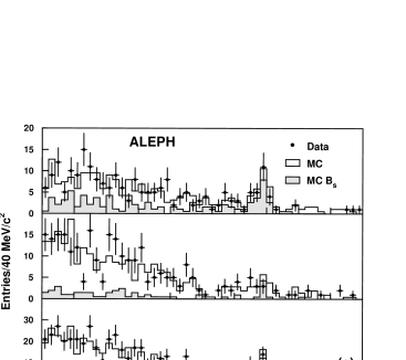
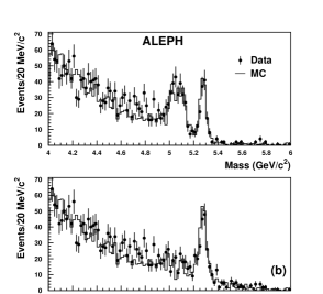
Figure 4: (a) Invariant mass distribution for candidates reconstructed in the ${\mathrm{D}}_{\mathrm{s}}^{-}\pi^{+}$ final state (top), ${\mathrm{D}}_{\mathrm{s}}^{-}{\mathrm{a}}_{1}^{+}$ final state (middle) and all channels together (bottom).
(b) Invariant mass distribution of ${\mathrm{B}}^{+}$ candidates before (top) and after (bottom) $\pi^{0}$ reconstruction.

Figure 5: (a) Invariant mass distribution of ${\mathrm{D}}_{\mathrm{s}}$ candidates in ${\mathrm{D}}_{\mathrm{s}}^{-}\ell^{+}$ combinations, reconstructed in hadronic final states.
(b) Mass distribution of the selected $\phi$ candidates in semileptonic ${\mathrm{D}}_{\mathrm{s}}$ decays.

Final states containing a ${\mathrm{D}}_{\mathrm{s}}\ell$ pair are reconstructed using several hadronic modes of the ${\mathrm{D}}_{\mathrm{s}}$, plus the decay mode ${\mathrm{D}}_{\mathrm{s}}^{-}\to\phi\ell^{-}$. The fraction of resonant component is estimated directly from the data, from the sidebands of the ${\mathrm{D}}_{\mathrm{s}}$ and $\phi$ mass peaks, shown in Fig. 5. A resonant background component is given by double-charm b decays ${\mathrm{b}}\to{\mathrm{D}}_{\mathrm{s}}^{\pm}{\mathrm{D}}(X)$ with ${\mathrm{D}}\to X\ell^{\mp}$. Such events are discriminated from the signal using lepton kinematics and jet topology: several variables are combined by means of a neural network, and the signal purity is estimated as a function of the discriminant, using simulated events.

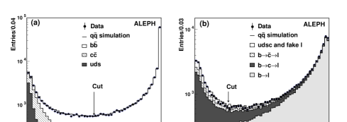
Figure 6: The b-tagging variable (a) and the ${\mathrm{b}}\to\ell$ tagging variable (b) distributions for the inclusive lepton candidates. Distribution of the ${\mathrm{B}}_{\mathrm{s}}$ purity variable $N_{\mathrm{pur}}$ (c), and fraction of each b-hadron species as a function of $N_{\mathrm{pur}}$ (d).

The analysis of inclusive semileptonic decays makes use of a novel algorithm for secondary vertex reconstruction. A ${\mathrm{D}}$ track is defined from the charged particles identified as decay products of the inclusively reconstructed ${\mathrm{D}}$ meson. The direction of such ${\mathrm{D}}$ track is improved by adding photons reconstructed in a cone around the ${\mathrm{D}}$ meson, and forming with it an invariant mass smaller than the nominal ${\mathrm{D}}$ mass. A ${\mathrm{B}}$ track is formed from the jet or the thrust axis direction, depending on the event topology, with angular uncertainties parameterized from the simulation. The lepton, the improved ${\mathrm{D}}$ track and the ${\mathrm{B}}$ track are fit together to find the ${\mathrm{B}}$ meson decay vertex. As mentioned in Section 2.3, estimates of the initial and final state tag performance, of the sample composition (Fig. 6), and, most importantly, of the uncertainty on the reconstructed decay length and momentum, are obtained for each event from parametrizations as a function of the relevant event properties.

For the three analyses, systematic uncertainties are calculated taking into account not only the change in the fitted amplitude, but also the change in its statistical uncertainty, which in some cases is more relevant. The method is based on toy experiments. The amplitude spectra obtained are shown in Fig. 7.

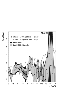
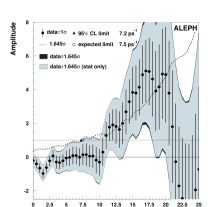
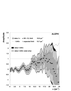
(a)                                       (b)                                       (c)

Figure 7: Fitted amplitude spectra for the fully reconstructed sample (a), the ${\mathrm{D}}_{\mathrm{s}}\ell$ sample (b) and the inclusive lepton sample (c).

5 Conclusions: the World combination

The combined amplitude spectrum from all available analyses  is shown in Fig. 8a. Frequencies smaller than $14.9~{}{\mathrm{ps}}^{-1}$ are excluded at 95% CL. The expected limit, $19.4~{}{\mathrm{ps}}^{-1}$, is substantially higher because amplitude values different from zero, and close to unity, are found in the frequency range $16-20~{}{\mathrm{ps}}^{-1}$. The structure observed is compatible with the hybothesis of an oscillation signal, as can be appreciated from the likelihood profile shown in Fig. 8b, but its statistical significance is smaller than two standard deviations, and is therefore insufficient to claim an observation.

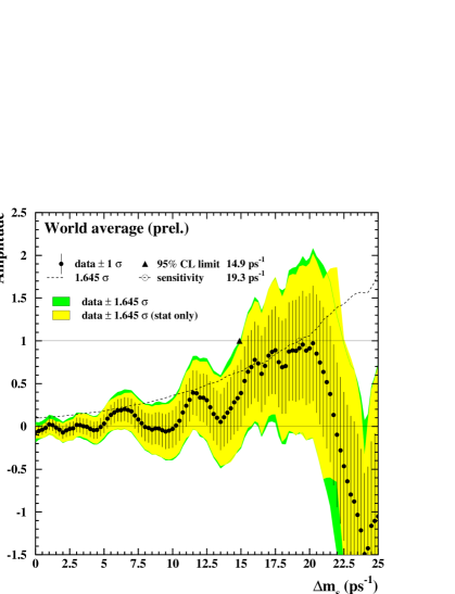
(a)                                                                                (b)

Figure 8: Amplitude spectrum for the combination of all available analyses (a), and corresponding log-likelihood profile (b); the dotted curve gives the expected likelihood depth at each frequency for $\omega=\Delta m_{\mathrm{s}}$.

Figure 9: (a) Uncertainty on the fitted amplitude as a function of test frequency, for the experiments that have performed ${\mathrm{B}}_{\mathrm{s}}$ oscillation searches.
(b) Weight of the different experiments in the combination.

The estimated uncertainty on the fitted amplitude as a function of test frequency is shown in Fig. 9a for the available analyses combined by experiment. In Fig. 9b the weight of each experiment in the world combination is shown. In the region $16-20{\mathrm{ps}}^{-1}$ where the deviation from ${\cal{A}}=0$ is observed, ALEPH and SLD dominate the combination.

6 Acknowledgements

I wish to thank the organizers for the interesting conference and the pleasant stay in La Thuile.

References

- 1 . H.G. Moser and A. Roussarie, Nucl. Instrum. Methods A 384, 491 (1997).
- 2 . D. Abbaneo and G. Boix, JHEP 08, 004 (1999).