First Measurement of $\Gamma(D^{\ast+})$ and
Precision Measurement of $m_{D^{\ast+}}-m_{D^{0}}$

Abstract

We present the first measurement of the $D^{\ast+}$ width using 9/fb of $e^{+}e^{-}$ data collected near the $\Upsilon(4\rm{S})$ resonance by the CLEO II.V detector. Our method uses advanced tracking techniques and a reconstruction method that takes advantage of the small vertical size of the CESR beam spot to measure the energy release distribution from the $D^{\ast+}\to D^{0}\pi^{+}$ decay. We find $\Gamma(D^{\ast+})=96\pm 4\ ({\rm Statistical})\pm 22\ ({\rm Systematic})$ keV. We also measure the energy release in the decay and compute $\Delta m\equiv m_{D^{\ast+}}-m_{D^{0}}=145.412\pm 0.002({\rm Statistical})\pm 0.012\ ({\rm Systematic})$ MeV/c².

I Introduction

A measurement of $\Gamma(D^{\ast+})$ opens an important window on the non-perturbative strong physics involving heavy quarks. The basic framework of the theory is well understood, however, there is still much speculation - predictions for the width range from $15\,\rm{keV}$ to $150\,\rm{keV}$ [1]. The level splitting in the $B$ sector is not large enough to allow real strong transitions. Therefore, a measurement of the width of the $D^{\ast+}$ gives unique information about the strong coupling constant in heavy-light meson systems.

The total width of the $D^{\ast+}$ is the sum of the partial widths of the strong decays $D^{\ast+}\to D^{0}\pi^{+}$ and $D^{\ast+}\to D^{+}\pi^{0}$ and the electromagnetic decay $D^{\ast+}\to D^{+}\gamma$. We can write the width in terms of strong couplings, $g_{D^{\ast}\to D^{0}\pi^{+}}$ and $g_{D^{\ast}\to D^{+}\pi^{0}}$, and an electromagnetic coupling, $g_{D^{\ast}\to D^{+}\gamma}$:

$$\Gamma(D^{\ast+}) = \Gamma(D^{0}\pi^{+})+\Gamma(D^{+}\pi^{0})+\Gamma(D^{+}\gamma)$$ (1)

$$= \frac{g_{D^{\ast}\to D^{0}\pi^{+}}^{2}}{24\pi m_{D^{\ast+}}^{2}}p^{3}_{\pi^{+}}+\frac{g_{D^{\ast}\to D^{+}\pi^{0}}^{2}}{24\pi m_{D^{\ast+}}^{2}}p^{3}_{\pi^{0}}+\frac{\alpha g_{D^{\ast}\to D^{+}\gamma}^{2}}{3}p^{3}_{\gamma},$$ (2)

where the momenta are those for the indicated particle in the $D^{\ast+}$ rest frame, and $\alpha$ is the fine structure constant. This can be rewritten using the isospin relationship

$$g_{D^{\ast}\to D\pi}=-\sqrt{2}g_{D^{\ast}\to D^{+}\pi^{0}}=g_{D^{\ast}\to D^{0}\pi^{+}},$$ (3)

and relating $g_{D^{\ast}\to D\pi}$ to a universal strong coupling between heavy vector and pseudoscaler mesons to the pion, $g$, with

$$g_{D^{\ast}\to D\pi}=\frac{2m_{D^{\ast}}}{f_{\pi}}g,$$ (4)

where $f_{\pi}$ is the pion decay constant. All this yields

$$\Gamma(D^{\ast+})=\frac{2g^{2}}{12\pi f_{\pi}^{2}}p^{3}_{\pi^{+}}+\frac{g^{2}}{12\pi f_{\pi}^{2}}p^{3}_{\pi^{0}}+\frac{\alpha g_{D^{\ast}\to D^{+}\gamma}^{2}}{3}p^{3}_{\gamma}.$$ (5)

The width of the $D^{\ast+}$ only depends on $g$ [2] since the contribution of the electromagnetic decay with branching fraction $(1.68\pm 0.45)$% [3] can be neglected. The measurement of $g$ is needed in the extraction of $V_{ub}$ in semileptonic $b\to u$ decays [4].

Prior to this measurement, the $D^{\ast+}$ width was limited to be less than $131\,\rm{keV}$ at the $90\%$ confidence level by the ACCMOR collaboration [5]. The limit was based on 110 signal events reconstructed in two $D^{0}$ decay channels with a background of 15%. This contribution describes a measurement of the $D^{\ast+}$ width with the CLEO II.V detector where the signal, in excess of 11,000 events, is reconstructed through a single, well-measured sequence, $D^{\ast+}\rightarrow\pi^{+}_{\rm slow}D^{0}$, $D^{0}\rightarrow K^{-}\pi^{+}$. Consideration of charge conjugated modes are implied throughout this paper. The level of background under the signal is less than 3% in our loosest selection.

The challenge of measuring the width of the $D^{\ast+}$ is understanding the tracking system response function since the experimental resolution exceeds the width we are trying to measure. Candidates with tracks that have mismeasured hits, errors in pattern recognition, and large angle Coloumb scattering are particularly dangerous because the signal shape they project is broad and the errors for these events can be underestimated, resulting in events that can easily influence the parameters of a Breit-Wigner fitting shape. We generically term such effects “tracking mishaps.” A difficulty is that there is no physical calibration for this measurement. The ideal calibration mode would have a large cross-section, a width of zero, decay with a rather small energy release to three charged particles one of which has a much softer momentum distribution than the other two which decay through a nearly zero width resonance with a measurable flight distance. Such a mode would allow us to disentangle detector effects from the underlying width but no such mode exists.

Therefore, to measure the width of the $D^{\ast+}$ we depend on exhaustive comparisons between a GEANT [6] based detector simulation and our data. We addressed the problem by selecting samples of candidate $D^{\ast+}$ decays using three strategies.

First we produced the largest sample from data and simulation by imposing only basic tracking consistency requirements. We call this the nominal sample.

Second we refine the nominal sample selecting candidates with the best measured tracks by making very tight cuts on tracking parameters. There is special emphasis on choosing those tracks that are well measured in our silicon vertex detector. This reduces our nominal sample by a factor of thirty and, according to our simulation, has negligible contribution from tracking mishaps. We call this the tracking selected sample.

A third alternative is to select our data on specific kinematic properties of the $D^{\ast+}$ decay that minimize the dependence of the width of the $D^{\ast+}$ on detector mismeasurements. The nominal sample size is reduced by a factor of three and a half and, again according to our simulation, the effect of tracking problems is reduced to negligible levels. We call this the kinematic selected sample.

In all three samples the width is extracted with an unbinned maximum likelihood fit to the energy release distribution and compared with the simulation’s generated value to determine a bias which is then applied to the data. These three different approaches yield consistent values for the width of the $D^{\ast+}$ giving us confidence that our simulation accurately models our data.

II CLEO Detector and Data Samples

The CLEO detector has been described in detail elsewhere. All of the data used in this analysis are taken with the detector in its II.V configuration [7]. This work mainly depends on the tracking system of the detector which consists of a three-layer, double sided silicon strip detector, an intermediate ten-layer drift chamber, and a large 51-layer helium-propane drift chamber. All three are in an axial magnetic field of 1.5 Tesla provided by a superconducting solenoid that contains the tracking region. The charged tracks are fit using a Kalman filter technique that takes into account energy loss as the tracks pass through the material of the beam pipe and detector [8].

The data were taken in symmetric $e^{+}e^{-}$ collisions at a center of mass energy around 10 GeV with an integrated luminosity of 9.0/fb provided by the Cornell Electron-positron Storage Ring (CESR). The nominal sample follows the selection of $D^{\ast+}\to\pi_{\rm slow}^{+}D^{0}\to K^{-}\pi^{+}\pi_{\rm slow}^{+}$ candidates used in our $D^{0}-\bar{D^{0}}$ mixing analysis[9].

Our reconstruction method takes advantage of the small CESR beam spot and the kinematics and topology of the $D^{\ast+}\to\pi^{+}_{\rm slow}D^{0}\to\pi^{+}_{\rm slow}K^{-}\pi^{+}$ decay chain. The $K^{-}$ and $\pi^{+}$ are required to form a common vertex. The resultant $D^{0}$ candidate momentum vector is then projected back to the CESR luminous region to determine the $D^{0}$ production point. The CESR luminous region has a Gaussian width $\sim 10\ \mu$m vertically and $\sim 300\ \mu$m horizontally. It is well determined by an independent method[10]. This procedure determines an accurate $D^{0}$ production point for $D^{0}$’s moving out of the horizontal plane; $D^{0}$’s moving within 0.3 radians of the horizontal plane are not considered. Then the $\pi_{\rm slow}^{+}$ track is refit constraining its trajectory to intersect the $D^{0}$ production point. This improves the resolution on the energy release, $Q=M(K^{-}\pi^{+}\pi_{\rm slow}^{+})-M(K^{-}\pi^{+})-m_{\pi^{+}}$, by more than 30% over simply forming the appropriate invariant masses of the tracks. The improvement to resolution is essential to our measurement of the width of the $D^{\ast+}$. Our resolution is shown in Figure 1

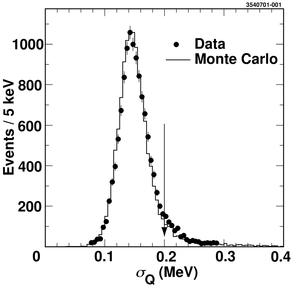
FIG. 1.: Distribution of $\sigma_{Q}$, the uncertainty on $Q$ as determined from propagating track fitting errors. The arrow indicates a selection discussed in the text.

and is typically 150 keV. The good agreement between Monte Carlo and data demonstrates that the kinematics and sources of uncertainties on the tracks, such as the number of hits used and the effects of multiple scattering in detector material, are well modeled.

To further improve the quality of reconstruction in our nominal sample, we apply some kinematic cuts to remove a small amount of misreconstructed signal and background. Figure 2 shows the distribution of the momentum

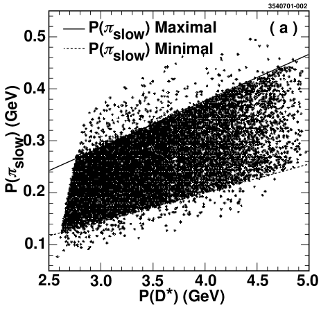
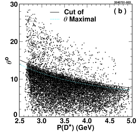
FIG. 2.: The $\pi_{\rm slow}^{+}$ momentum (a) and the opening angle between $D^{0}$ and $\pi_{\rm slow}^{+}$ (b) both versus the $D^{\ast+}$ momentum in the nominal data sample.

of the $\pi_{\rm slow}^{+}$ as a function of the $D^{\ast+}$ candidate momentum. We apply a cut at the kinematic boundary as shown in the figure. Figure 2 also shows the opening angle $\theta$ between the $\pi_{\rm slow}^{+}$ and the $D^{0}$ candidate as a function of the $D^{\ast+}$ candidate momentum. We apply a cut of $\theta<38^{\circ}/P_{D^{\ast}}[{\rm GeV}]$ which is just beyond the kinematic limit to account for resolution smearing. We also require $\sigma_{Q}<200$ keV which removes the long tail in the error distribution.

The tracking selected sample makes much more stringent cuts on the quality of the tracks used to identify the candidates. All tracks are required to have hits in both the $r\phi$ and $z$ views in all three layers of the silicon strip detector as opposed to the nominal two silicon hits per view. None of these hits are allowed to be within 2 mm of a silicon wafer edge. The $D^{0}$ daughter tracks are required to have at least 38 of the possible 51 main drift chamber hits and seven of the ten intermediate drift chamber hits. The $\chi^{2}$ per degree of freedom of the fit to these two tracks are limited to less than 2 in each of the two drift chambers and 50 in the silicon strip detector. These selections are designed to remove tracks that have tracking mishaps or decay in flight.

We compare the simulation and the data as a function of kinematic variables of the $D^{\ast+}$ decay. This will provide another test of the simulation’s modeling of the data, and be the basis of our study of systematic uncertainties in the analysis. The most important kinematic variables are the “derivatives” which are defined by

$$M^{2}=M(K\pi)^{2}+m^{2}_{\pi^{+}_{\rm slow}}+2(E_{D^{0}}E_{\pi^{+}_{\rm slow}}-p_{D^{0}}p_{\pi^{+}_{\rm slow}}\cos\theta)\ ,$$ (6)

$$\beta_{D^{0}}=p_{D^{0}}/E_{D^{0}},$$ (7)

$$\beta_{\pi^{+}_{\rm slow}}=p_{\pi^{+}_{\rm slow}}/E_{\pi^{+}_{\rm slow}},$$ (8)

$$\frac{\partial Q}{\partial P_{D^{0}}} \equiv \frac{E_{\pi^{+}_{\rm slow}}}{M}(\beta_{D^{0}}-\beta_{\pi^{+}_{\rm slow}}\cos\theta),$$ (9)

$$\frac{\partial Q}{\partial P_{\pi^{+}_{\rm slow}}} \equiv \frac{E_{D^{0}}}{M}(\beta_{\pi^{+}_{\rm slow}}-\beta_{D^{0}}\cos\theta),$$ (10)

$$\frac{\partial Q}{\partial\theta} \equiv \frac{p_{D^{0}}p_{\pi^{+}_{\rm slow}}}{M}\sin\theta.$$ (11)

These derivatives test correlations among the basic kinematic variables, the $D^{0}$ and $\pi^{+}_{\rm slow}$ momenta and the opening angle, $\theta$. We compare by dividing the $Q$ distribution into ten slices in each of the kinematic variables and fitting the ten sub-distributions of $Q$ to Gaussians. We display the width and mean of the ten fits as a function of each of the six kinematic variables in Figures 3 and 4.

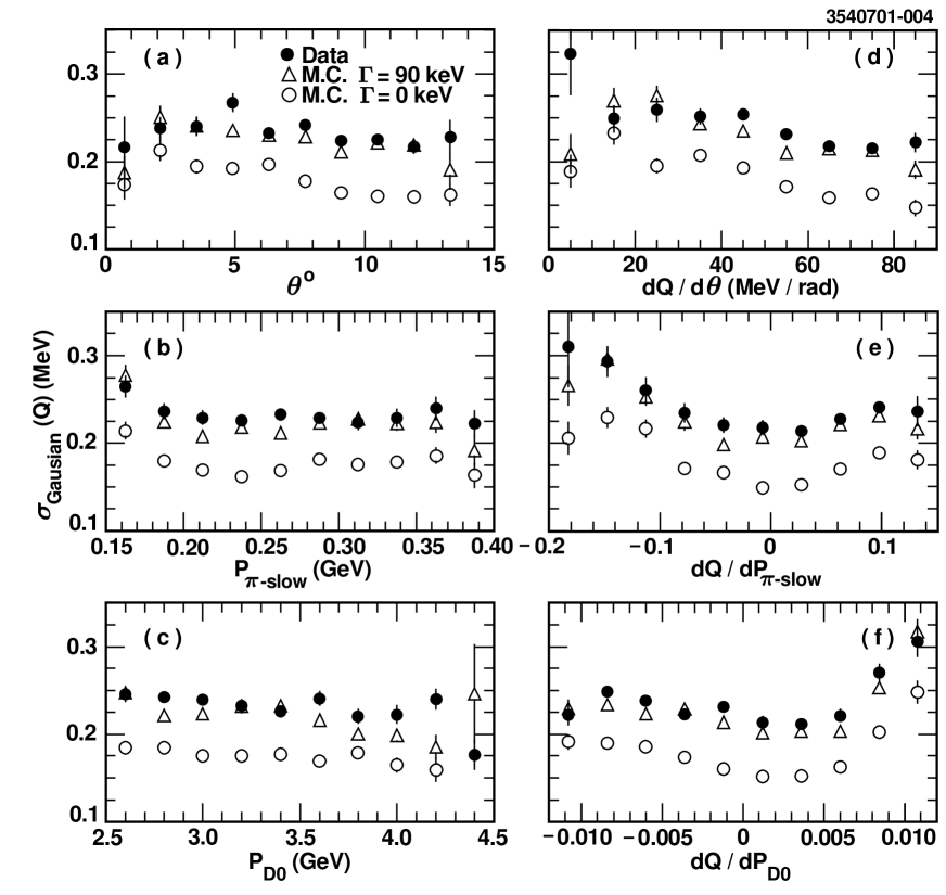
FIG. 3.: Gaussian width of $Q$ distribution versus kinematic parameters and derivatives. $\bullet$ – Data; $\circ$–Simulation with $\Gamma_{D^{\ast}+}=0$; $\triangle$–Simulation with $\Gamma_{D^{\ast}+}=90$ keV.

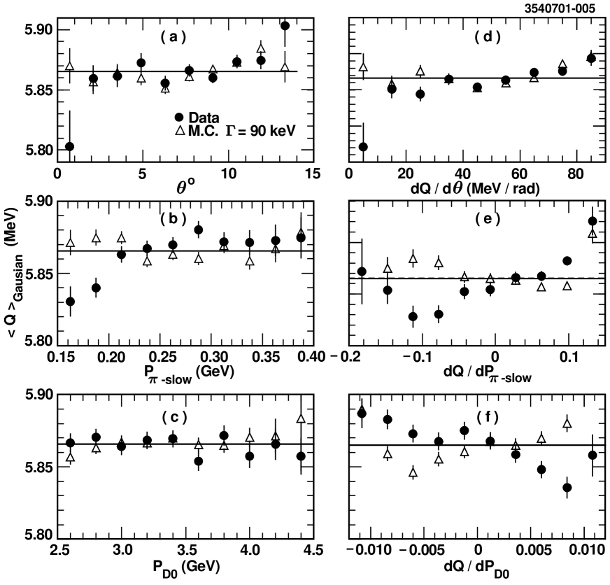
FIG. 4.: Gaussian mean of $Q$ distribution versus kinematic parameters and derivatives. $\bullet$–Data; $\triangle$–Simulation with $\Gamma_{D^{\ast}+}=90$ keV. The horizontal lines show the average value of $Q$ for the two samples.

The quality of the width comparison (Figure 3) is excellent, with the simulation generated with an underlying $\Gamma(D^{\ast+})$ in the range of 90–100 keV agreeing well with the data for all the kinematic variables. Even when generated with an underlying $\Gamma(D^{\ast+})=0$ keV the simulation accurately follows the data’s changes as the kinematic variables vary across their allowed range.

The quality of the mean comparison (Figure 4) is not as good. The dependence of the mean of $Q$ is not well modeled versus the $\pi^{+}_{\rm slow}$ momentum, $\partial Q/\partial P_{\pi^{+}_{\rm slow}}$, and $\partial Q/\partial P_{D^{0}}$ by our simulation. We discuss the consequences of this imperfect modeling of the data in the section on systematic uncertainties below.

Figure 5 shows

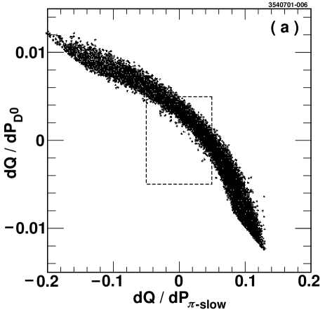
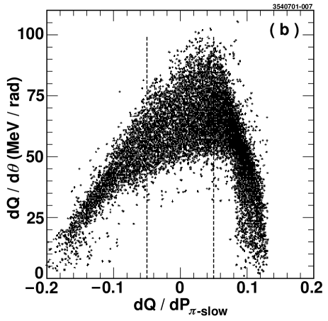
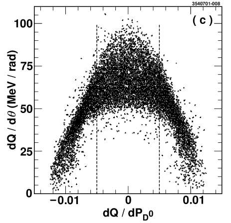
FIG. 5.: Distributions of $\partial Q/\partial P_{D^{0}}$ versus $\partial Q/\partial P_{\pi^{+}_{\rm slow}}$ (a), $\partial Q/\partial\theta$ versus $\partial Q/\partial P_{\pi^{+}_{\rm slow}}$ (b), and $\partial Q/\partial\theta$ versus $\partial Q/\partial P_{D^{0}}$ (c) in the data. The dashed regions show the selection that defines the kinematic selected sample.

the three derivatives plotted against each other in the data. Note that if we select $\partial Q/\partial P_{D^{0}}$ and $\partial Q/\partial P_{\pi^{+}_{\rm slow}}$ both to be close to zero we minimize the dependence of $Q$ on the basic kinematic variables $P_{D^{0}}$ and $P_{\pi^{+}_{\rm slow}}$, and thus minimize the contribution of the kinematic variables to the width of the $Q$ distribution. With this selection we are more sensitive to the underlying width of the $Q$ distribution rather than variations caused by any mismodeling of $Q$’s dependence on the basic kinematics. The kinematic selection is defined by

$$\left|\frac{\partial Q}{\partial P_{D^{0}}}\right| \leq 0.005,$$ (12)

$$\left|\frac{\partial Q}{\partial P_{\pi^{+}_{\rm slow}}}\right| \leq 0.05.$$ (13)

Table III summarizes the statistics in our three samples. The tracking and kinematic samples are subsets of the nominal sample. The two subsets contain 94 common candidates.

III Fit Description

We assume that the intrinsic width of the $D^{0}$ is negligible, $\Gamma(D^{0})\ll\Gamma(D^{\ast+})$, implying that the width of $Q$ is simply a convolution of the shape given by the $D^{\ast+}$ width and the tracking system response function. Thus we consider the pairs of $Q$ and $\sigma_{Q}$ for $D^{\ast+}\to\pi_{\rm slow}^{+}D^{0}\to K^{-}\pi^{+}\pi_{\rm slow}^{+}$ where $\sigma_{Q}$ is given for each candidate by propagating the tracking errors in the kinematic fit of the charged tracks. We perform an unbinned maximum likelihood fit to the $Q$ distribution.

The underlying signal shape of the $Q$ distribution is assumed to be given by a P-wave Breit-Wigner with central value of $Q$, $Q_{0}$. We considered a relativistic and non-relativistic Breit-Wigner as a model of the underlying signal shape, and found negligible changes in the fit parameters between the two. The width of the signal Breit-Wigner depends on $Q$ and is given by

$$\Gamma(Q)=\Gamma_{0}\left(\frac{P}{P_{0}}\right)^{3}\left(\frac{M_{0}}{M}\right)^{2},$$ (14)

where $\Gamma_{0}$ is equivalent to $\Gamma(D^{\ast+})$, $P$ and $M$ are the candidate $\pi_{\rm slow}^{+}$ or $D^{0}$ momentum in the $D^{\ast+}$ rest frame and $K\pi\pi_{\rm slow}$ mass, and $P_{0}$ and $M_{0}$ are the values computed using $Q_{0}$. The effect of the mass term is negligible at our energy. The partial width and the total width differ negligibly in their dependence on $Q$ for $Q>1~{}MeV$.

For each candidate the signal shape is convolved with a resolution Gaussian with width $\sigma_{Q}$, determined by the tracking errors, as a model of our finite resolution shown in Figure 1.

The fit also includes a background contribution with a fixed shape. The shape for the background is taken from fits to the background prediction of our simulation with a third order polynomial. The level of the background is allowed to float in our standard fit. The predicted background shape and fits are displayed in Figure 6.

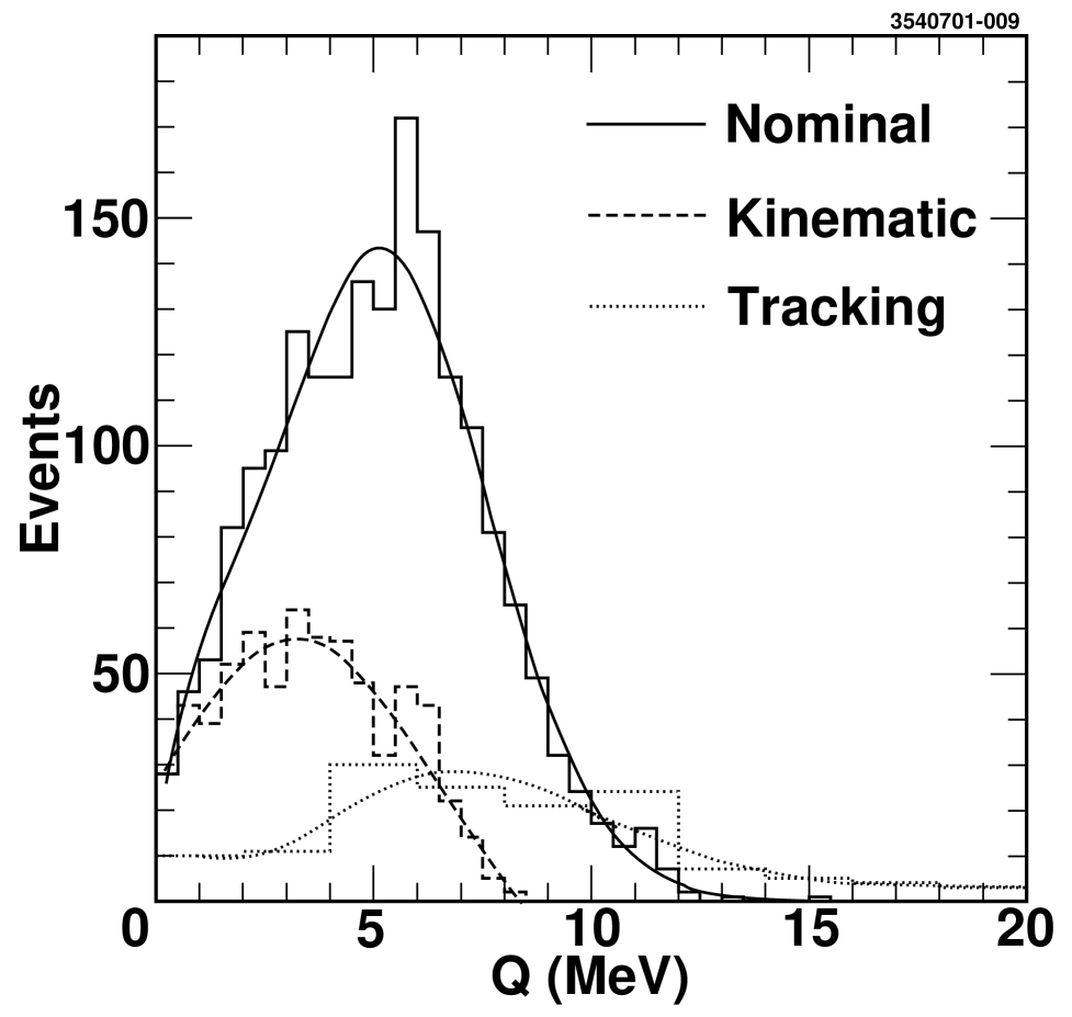
FIG. 6.: Our simulation’s prediction of the background for the three samples discussed in the text. Also shown are the fits to third order polynomials that are used in the fits to the data.

Figure 7 shows the $Q$ distribution for

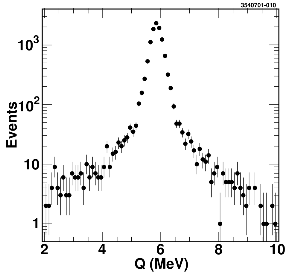
FIG. 7.: The $Q$ distribution of the nominal sample in the data.

our nominal data sample. Note that besides the well measured signal and the small, slowly varying background, there is also a small component centered on the signal with a large width. Therefore we allow a small fraction of the signal, $f_{mis}$, to be parametrized by a single Gaussian resolution function of width $\sigma_{mis}$. This shape is included in the fit to model the tracking mishaps which our simulation predicts to be at the 5% level in the nominal sample and negligible in both the tracking and kinematic selected samples. Typically we constrain the level of this contribution while allowing $\sigma_{mis}$ to float.

We have many other parameters of the fit that can be varied or allowed to float for testing purposes. We can allow a scale factor on each candidate’s $\sigma_{Q}$ to model a systematic mistake in our tracking system caused, for example, by not properly accounting for the material of the detector. In our standard fits we only allow the normalization of the background to float, but we can either vary the shape as indicated by the simulation or allow the parameters of the background polynomial to float as a measure of the small systematic uncertainty due to the background shape.

Table I summarizes the parameters of our

TABLE I.: Parameters of our fit to the $Q$ distribution

Parameter	Description
$\Gamma_{0}$	Breit Wigner width of $Q$ signal distribution, $\Gamma(D^{\ast+})$
$Q_{0}$	Mean of $Q$ signal distribution
$N_{s}$	Number of signal events
$f_{mis}$	Fraction of mismeasured signal
$\sigma_{mis}$	Resolution on measured $Q$ for mismeasured signal
$N_{b}$	Number of background events
$k$	$\sigma_{Q}$ scale factor, fixed to 1
$B_{1,2,3}$	Coefficients of background polynomial, fixed from simulation

fit. Note that the $\sigma_{Q}$ scale factor $k$ and the background shape parameters $B_{1,2,3}$ are fixed in our nominal fits. We minimize the likelihood function

$$L=2(N_{s}+N_{b})-2\sum_{i=1}^{N}\log[N_{s}S(Q_{i},\sigma_{Qi};\Gamma_{0},Q_{0},f_{mis},\sigma_{mis},k)+N_{b}B(Q_{i};B_{1,2,3})],$$ (15)

where $S$ and $B$ are respectively the signal and background shapes discussed above.

The fitter has been extensively tested both numerically and with input from our full simulation. We find that the fitter performs reliably giving normal distributions for the floating parameters and their uncertainties. It also reproduces the input $\Gamma(D^{\ast+})$ from 0 to 130 keV. Its behavior on each of the three data samples: nominal; tracking selected; and kinematic selected in the full simulation is discussed below. We note that if all the parameters are allowed to vary simultaneously there is strong correlation among the intrinsic width, $\Gamma_{0}$, the fraction of mismeasured events, $f_{mis}$, and the $\sigma_{Q}$ scale factor, $k$, as one would expect. Thus our nominal fit holds $k$ fixed, but in our systematic studies we either fix one of the three or provide a constraint with a contribution to the likelihood if the parameter varies from its nominal value.

IV Fit Results

As a preliminary test to fitting the data we run the complete analysis on a fully simulated sample that has about ten times the data statistics and is generated with a range of underlying $\Gamma(D^{\ast+})$ from 0 to 130 keV. We do this for nominal, tracking, and kinematic selected samples. For the nominal sample we note that the fit is not stable if all the parameters are left to vary freely. We have found that if we constrain the fraction of mismeasured signal to $(5.3\pm 0.5)$% as indicated by the simulation over the range of generated widths of the $D^{\ast+}$ then we get a stable result. This constraint makes the fit to the simulated nominal sample have no significant offset between the generated and measured values for the width of the $D^{\ast+}$. The tracking and kinematic selected samples have a negligible amount of mismeasured signal according to the simulation and in fits to these samples we fix $f_{mis}$ to zero. These simulated samples are also consistent with no offset between the generated and measured values for the width of the $D^{\ast+}$. We also note that in all three simulated samples there are no trends in the difference between measured and generated width as a function of the generated width; the offset is consistent with zero as a function of the generated width of the $D^{\ast+}$. Table III summarizes this simulation study. We will apply these offsets to the fit value that we obtain from the data. For the energy release all samples show small shifts, $-7\pm 3$ keV for the nominal, $-12\pm 10$ keV for the tracking, and $-12\pm 5$ keV for the kinematic.

Figures 8, 9, and 10

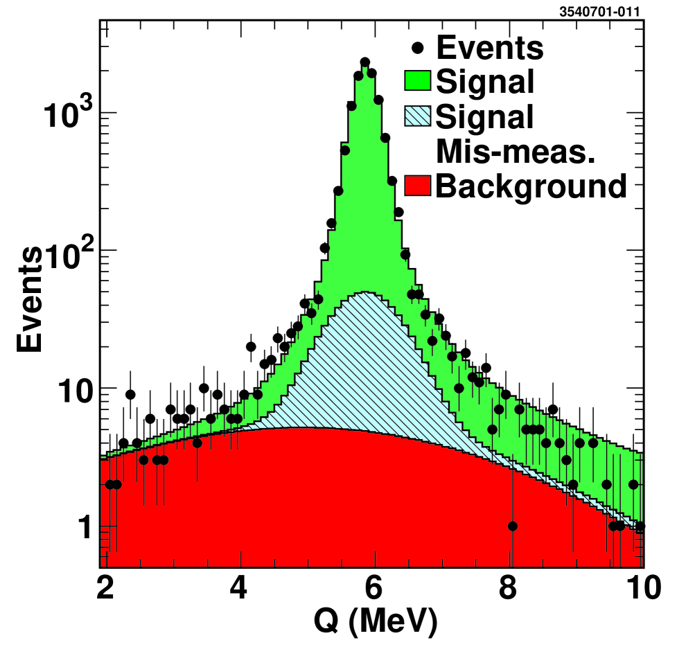
FIG. 8.: Fit to nominal data sample. The different contributions to the fit are shown by different colors.

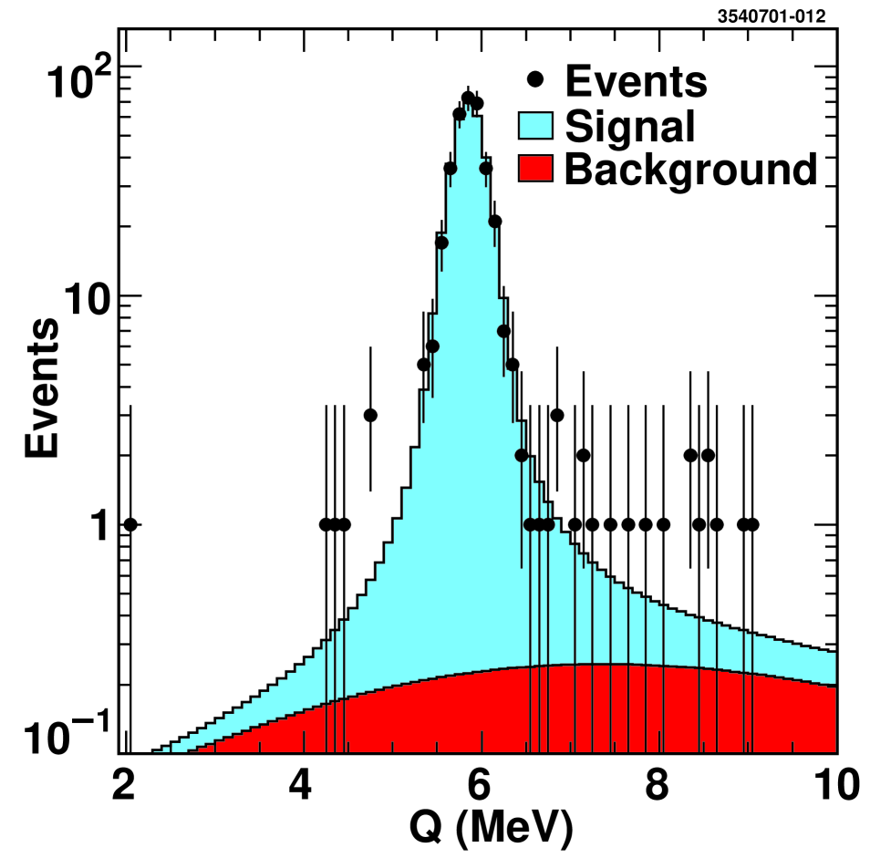
FIG. 9.: Fit to tracking selected data sample. The different contributions to the fit are shown by different colors.

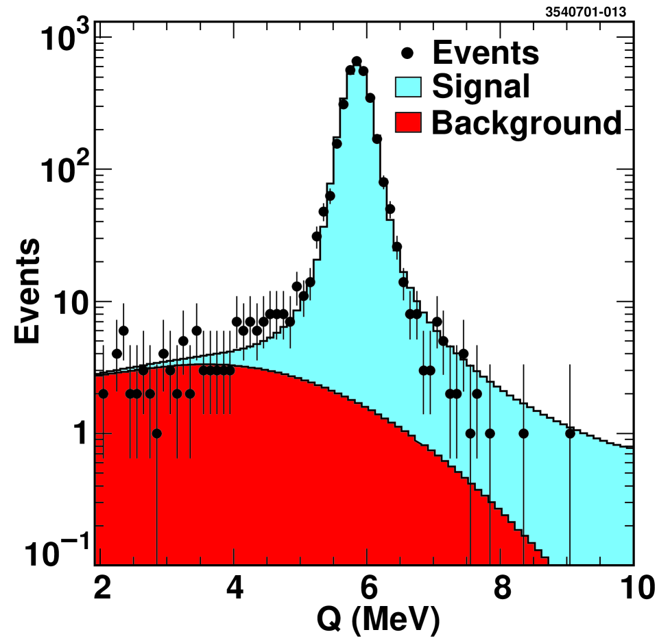
FIG. 10.: Fit to kinematic selected data sample. The different contributions to the fit are shown by different colors.

respectively display the fit to the nominal, tracking, and kinematic selected data samples. The results of the fits are summarized in Table II.

TABLE II.: Results of the fits described in the text. The fit parameters are summarized in Table I. The uncertainties are statistical.

	Sample
Parameter	Nominal	Tracking	Kinematic
$\Gamma_{0}$ (keV)	$98.9\pm 4.0$	$106.0\pm 19.6$	$108.1\pm 5.9$
$Q_{0}$ (keV)	$5853\pm 2$	$5854\pm 10$	$5850\pm 4$
$N_{s}$	$11207\pm 109$	$353\pm 20$	$3151\pm 57$
$f_{mis}$ (%)	$5.3\pm 0.5$	NA	NA
$\sigma_{mis}$ (keV)	$508\pm 39$	NA	NA
$N_{b}$	$289\pm 31$	$15\pm 7$	$133\pm 16$

Correlations among the floating parameters of the fit are negligible. Figure 11

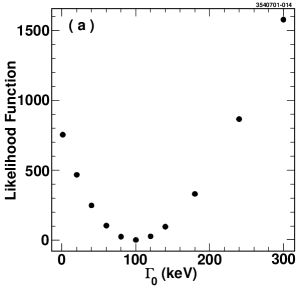
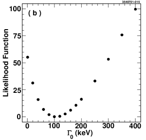
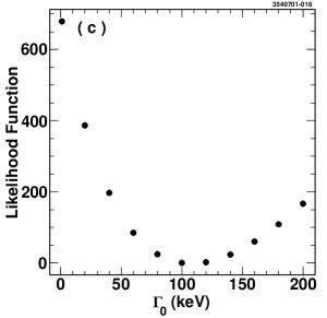
FIG. 11.: Likelihood function versus measured $D^{\ast+}$ width for the nominal (a), tracking (b), and kinematic (c) selected data samples.

displays the likelihood as a function of the width of the $D^{\ast+}$ for the fits to the three data samples.

The agreement is excellent among the three fits, and when the offsets from Table III are applied we obtain

$${\rm Nominal\ Sample} \Gamma(D^{\ast+})=96.2\pm 4.0\ {\rm keV},$$ (16)

$${\rm Tracking\ Selected} \Gamma(D^{\ast+})=104\pm 20\ {\rm keV},{\rm and}$$ (17)

$${\rm Kinematic\ Selected} \Gamma(D^{\ast+})=103.8\pm 5.9\ {\rm keV}.$$ (18)

The data sample and results are summarized in Table III.

TABLE III.: Summary of the data sample, simulation biases, and fit results.

	Sample
Parameter	Nominal	Tracking	Kinematic
Candidates	11496	368	3284
Background Fraction (%)	$2.51\pm 0.27$	$4.1\pm 1.9$	$4.05\pm 0.49$
$\Gamma_{\rm fit}-\Gamma_{\rm generated}$ (keV)	$2.7\pm 2.1$	$1.7\pm 6.4$	$4.3\pm 3.1$
Fit $\Gamma_{0}$ (keV)	$98.9\pm 4.0$	$106.0\pm 19.6$	$108.1\pm 5.9$
$D^{\ast+}$ Width (keV)	$96.2\pm 4.0$	$104\pm 20$	$103.8\pm 5.9$

The uncertainties are only statistical. We discuss systematic uncertainties in the next section.

V Systematic Uncertainties

We discuss the sources of systematic uncertainties on our measurements of the width of the $D^{\ast+}$ in the order of their size. The most important contribution is the variation of the results as a function of the kinematic parameters of the $D^{\ast+}$ decay as shown most clearly in Figure 4. We estimate this uncertainty by repeating the fits described above in three bins for each of the six kinematic parameters and taking the uncertainty as the largest observed variation from the nominal values in Table II. We obtain uncertainties of $\pm 16$ and $\pm 8$ keV on $\Gamma(D^{\ast+})$ and $Q_{0}$ respectively.

The next most important contribution comes from any mismodeling of $\sigma_{Q}$’s dependence on the kinematic parameters. We estimate this by varying our cut on $\sigma_{Q}$ from 75 to 400 from the nominal 200 keV and repeating our analysis with all parameters fixed except allowing the error scale factor $k$ to vary freely. This indicates that the resolution is correct to $\pm 4$%, and we then repeat our standard analysis with $k$ fixed at 0.96 and 1.04. We find uncertainties of $\pm 11$, $\pm 9$, and $\pm 7$ keV on $\Gamma(D^{\ast+})$ for the nominal, tracking, and kinematic selected sample. For $Q_{0}$ this uncertainty is negligible except in the tracking selected sample where it is $\pm 4$ keV.

We take into account correlations among the less well measured parameters of the fit, such as $k$, $f_{mis}$, and $\sigma_{mis}$, by fixing each parameter at $\pm 1\sigma$ from their central fit values, repeating the fit, and adding in quadrature the variation in the width of the $D^{\ast+}$ and $Q_{0}$ from their central values. We find uncertainties of $\pm 8$, $\pm 9$, and $\pm 9$ keV on the width of the $D^{\ast+}$ for the nominal, tracking, and kinematic selected sample, and respectively $\pm 3$, $\pm 4$, and $\pm 5$ keV on $Q_{0}$.

We have studied in the simulation the sources of mismeasurement that give rise to the resolution on the width of the $D^{\ast+}$ by replacing the measured values with the generated values for various kinematic parameters of the decay products. We have then compared these uncertainties with analytic expressions for the uncertainties. The only source of resolution that we cannot account for in this way is a small distortion of the kinematics of the event caused by the algorithm used to reconstruct the $D^{0}$ origin point described above. This contributes an uncertainty $\pm 4$ keV on the width of the $D^{\ast+}$ and $\pm 2$ keV on $Q_{0}$. We have also checked that our simulation accurately models the line shape of other narrow resonances visible in our data. Notably the decay $\Lambda^{0}\to p\pi^{-}$, has a $Q$ only seven times that of $D^{\ast+}\to D^{0}\pi^{+}_{\rm slow}$. In the $\Lambda^{0}$ decay we select the $\pi^{-}$ to have a momentum in the range of those in the $D^{\ast+}$ decay, and the visible widths agree to a few percent between data and simulation.

We consider uncertainties from the background shape by allowing the coefficients of the background polynomial to float. We observe changes on the width of $\pm 4$ keV for the nominal sample and $\pm 2$ keV for the tracking and kinematic selected samples. We have also released our kinematic selection cuts which causes the background to increase by a large factor. This causes a change which is small compared to allowing the coefficients of the background shape polynomial to float. Variations in the background have a negligible effect on $Q_{0}$.

Minor sources of uncertainty are from the width offsets derived from our simulation and given in Table III, and our digitized data storage format which saves track parameters with a resolution of 1 keV and contributes an uncertainty of $\pm 1$ keV on the width of the $D^{\ast+}$ and $Q_{0}$.

An extra and dominant source of uncertainty on $Q_{0}$ is the energy scale of our measurements. We evaluate this uncertainty by selecting $K_{s}\to\pi^{+}\pi^{-}$ decays in our data. The daughters tracks of the $K_{s}$ candidates are required to pass the same selection criterion as those described above in the nominal sample, the decay vertex is required to be inside the beam pipe, and the vertex is required to be significantly separated from the overall event vertex. Our $K_{s}$ sample is quite clean, less than 1% background under the mass peak, and has millions of candidates. We then plot the mean of the $\pi^{+}\pi^{-}$ invariant mass as function of the momentum of the daughters. We find that above a daughter momentum of 500 MeV/c the $K_{s}$ mass agrees with its expected value [11]. We apply corrections, less than 0.3% relative, to tracks between 100 and 500 MeV/c to bring the mass peaks into agreement with the nominal value. These corrections only affect the slow pion and produce a shift in $Q_{0}$ of $-4$ keV and a negligible change in the width. We evaluate uncertainties in the energy scale by varying an overall momentum scale to give a $\pm 30$ keV variation, the uncertainty, of the $K_{s}\to\pi^{+}\pi^{-}$ mass, and applying the statistical errors we obtain from the calculations of the momentum corrections discussed above. Conservatively we add in quadrature twice the observed shift. We observe an uncertainty of 8 keV on $Q_{0}$ and 1 keV on the width due to uncertainty in the energy scale of our measurements.

Table IV summarizes the systematic

TABLE IV.: Systematic uncertainties on the width of the $D^{\ast+}$ and $Q_{0}$

	Uncertainties in keV
	Sample
	Nominal		Tracking		Kinematic
Source	$\delta\Gamma(D^{\ast+})$	$\delta Q_{0}$	$\delta\Gamma(D^{\ast+})$	$\delta Q_{0}$	$\delta\Gamma(D^{\ast+})$	$\delta Q_{0}$
Dependence on Kinematics	16	8	16	8	16	8
Mismodeling of $\sigma_{Q}$	11	$<1$	9	4	7	$<1$
Fit Correlations	8	3	9	4	9	5
Vertex Reconstruction	4	2	4	2	4	2
Background Shape	4	$<1$	2	$<1$	2	$<1$
Offset Correction	2	3	6	10	3	5
Energy Scale	1	8	1	8	1	8
Data Digitization	1	1	1	1	1	1
Quadratic Sum	22	12	22	16	20	14

uncertainties on the width of the $D^{\ast+}$ and $Q_{0}$.

VI Conclusion

We have measured the width of the $D^{\ast+}$ by studying the distribution of the energy release in $D^{\ast+}\to D^{0}\pi^{+}$ followed by $D^{0}\to K^{-}\pi^{+}$ decay. We have done this in three separate samples, one that is minimally selected, a second that reduces poorly measured tracks due to misassociated hits and non-Gaussian scatters in the detector material, and a third that takes advantage of the kinematics of the decay chain to reduce dependence on mismeasurements of kinematic parameters. The resolution on the energy release is well modeled by our simulation, with agreement between the sources of the resolution as predicted by the simulation and analytic calculations. The largest sources of uncertainty are imperfect modeling of the dependence of the mean energy release on the kinematics of the decay chain, the simulation of the error on the energy release, and correlations among the parameters of the fit to the energy release distribution. With our estimate of the systematic uncertainties for each of the three samples being essentially the same we chose to report the result for the sample with the smallest statistical uncertainty, the minimally selected sample, and obtain

$$\Gamma(D^{\ast+})=96\pm 4\pm 22\ {\rm keV},$$ (19)

where the first uncertainty is statistical and the second is systematic. We note that if we form an average value taking into account the statistical correlations among our three measures we get a result that is nearly identical with Equation 19 since the average is dominated by the result with the smallest statistical uncertainty.

This is the first measurement of the width of the $D^{\ast+}$, and our measurement corresponds to a strong coupling[1]

$$g=0.59\pm 0.01\pm 0.07,$$ (20)

and

$$g_{D^{\ast}\to D\pi}=17.9\pm 0.3\pm 1.9.$$ (21)

This is consistent with theoretical predictions based on HQET and relativistic quark models, but higher than predictions based on QCD sum rules.

We also measure the mean value for the energy release in $D^{\ast+}\to D^{0}\pi^{+}$ decay

$$Q_{0}=5842\pm 2\pm 12\ {\rm keV},$$ (22)

where the first error is statistical and second is systematic. Combining this with the mass of the charged pion, 139.570 MeV, with an uncertainty less than 1 keV [11], we calculate

$$m_{D^{\ast}(2010)^{+}}-m_{D^{0}}=145.412\pm 0.002\pm 0.012\ {\mathrm{M}eV}.$$ (23)

This agrees with the value from the Particle Data Group, $145.436\pm 0.016$ MeV, from a global fit of all flavors of $D^{\ast}$–$D$ mass differences. It also agrees well with the best previous measure from a single experiment that includes an evaluation of systematic uncertainties from ACCMOR at $145.39\pm 0.07$ MeV [5].

REFERENCES

- [1] V.M.Belyaev et al. Phys. Rev. D 51, 6177 (1995) contains a recent survey summarizing and referencing previous theoretical work. P. Singer Acta Phys. Polon. B30 3849 (1999), J. L. Goity and W. Roberts JLAB-THY-00-45 (hep-ph/0012314), K. O. E. Henriksson, et al. Nuc. Phys. A 686, 355 (2001), and M. Di Pierro and E. Eichten hep-ph/0104208 appear since that survey.
- [2] M. Wise, Phys. Rev. D 45, R2188 (1992), G. Burdman and J. F. Donoghue, Phys. Lett. B 280, 287 (1992), and T. Yan et al., Phys. Rev. D 46, 1148 (1992) [Erratum-ibid. D 55, 5851 (1992)]. D. Becirevic and A. L. Yaouanc, JHEP 9903, 021 (1999) contains a recent review referencing previous theoretical work.
- [3] J.Bartelt et al. (CLEO Collaboration), Phys. Rev. Lett. 80, 3919, (1998).
- [4] G. Burdman, Z. Ligeti, M. Neubert and Y. Nir, Phys. Rev. D 49, 2331 (1994).
- [5] S.Barlag et al., Phys. Lett. B 278, 480 (1992).
- [6] R. Brun et al., GEANT3 Users Guide, CERN DD/EE/84-1.
- [7] Y. Kubota et al., (CLEO Collaboration), Nucl. Instrum. Methods Phys. Res., Sect. A 320, 66 (1992); T. Hill, Nucl. Instrum. Methods Phys. Res., Sect. A 418, 32 (1998).
- [8] P. Billior, Nucl. Instrum. Methods Phys. Res., Sect. A 225, 352 (1984).
- [9] R. Godang et al. (CLEO Collaboration), Phys. Rev. Lett. 84,5038 (2000)
- [10] D. Cinabro et al., CLNS 00/1706, physics/0011075.
- [11] D. E. Groom et al. (Particle Data Group), Eur.Phys.J. C 15, 1 (2000).