Electron Identification in Belle

Abstract

We report on electron identification methods and their performance in the Belle experiment at the KEK-B asymmetric B-Factory $e^{+}e^{-}$ storage ring. Electrons are selected using a likelihood approach that takes information from the electromagnetic calorimeter, the central drift chamber, and the silica aerogel Cherenkov counters as input. We achieve an electron identification efficiency of $(92.4\pm 0.4)\%$ with a $\pi^{\pm}$ fake rate of $(0.25\pm 0.02)\%$ for the momentum range between 1.0 GeV/$c$ and 3.0 GeV/$c$ in laboratory frame.

, , , and

1 Introduction

The primary goal of the Belle experiment, which is conducted at the KEK-B asymmetric $e^{+}$ (3.5 GeV) $e^{-}$ (8.0 GeV) collider, is to measure the $CP$ violation parameter $\sin 2\phi_{1}$ in the neutral $B$ meson system [1]. This measurement is done by studying the time evolution of events of the form $e^{+}e^{-}\rightarrow\Upsilon(4S)\rightarrow B^{0}\overline{B^{0}}$ where one $B^{0}$ decays to a $CP$ eigenstate (for example $B^{0}\rightarrow J/\Psi K_{S}$) and the other decays to a final state that reveals its “flavor” [2]. In this context “flavor” refers to whether the non-$CP$-eigenstate decay particle (the “tagging” $B^{0}$) is a $B^{0}$ or a $\overline{B^{0}}$. Electron identification (EID), which includes both $e^{+}$ and $e^{-}$, plays an important role in this measurement since one of the most reliable methods of determining a $B^{0}$ meson’s flavor is to observe the sign of the charged lepton that emerges when it undergoes semi-leptonic decay.

In addition, EID is useful for reconstructing the large class of $CP$ eigenstates that involve final-state $J/\Psi$ particles, since these are detected via the decay $J/\Psi\rightarrow\ell^{+}\ell^{-}$ where electron and muon pairs occur in equal numbers.

Moreover, EID is crucial for analyses of $b\rightarrow c$ (or $u$) $e^{-}\bar{\nu}$ semileptonic decays, which enable us to extract $V_{cb}$ or $V_{ub}$ [3]. For these purposes, electrons with the laboratory momenta above 1 GeV/$c$ and below 3 GeV/$c$ must be identified with high efficiency and high purity.

This paper describes the method used to discriminate between electrons and other charged particles (mostly pions). Its performance will also be given. In Section 2 , a brief description of the Belle detector is given. In Section 3 the details of the EID technique are presented and in Sections 4 and 5 the performance results in terms of efficiency and fake rate are reported. The last section concludes this study.

2 The Detector

The Belle detector, which is shown in Fig. 1, consists of a silicon vertexing detector for precise vertex finding, a central drift chamber (CDC) for detecting charged particles, arrays of silica aerogel Cherenkov counters (ACC) for particle identification and time of flight counters for particle identification, an electromagnetic calorimeter (ECL) for photon and electron detection, a system of resistive plate chambers interspersed with the magnetic return yoke for $\mu/\mbox{$K_{L}$}$ detection (KLM), and an extreme forward calorimeter for online luminosity measurement.

A 1.5-T magnetic field is excited by a superconducting solenoid situated between the ECL and the KLM. Additional details of the detector can be found in [4]. The sub-detectors relevant to EID are briefly described below.

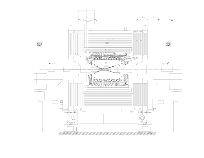
Figure 1: Plan view of the Belle detector.

The CDC is a cylindrical chamber with the inner radius of 77 mm, outer radius of 880 mm, and a length of 2400 mm. The geometrical coverage in $\theta$ is $17^{\circ}<\theta<150^{\circ}$ . In addition to the tracking, the $dE/dx$ measurement that is made by the CDC plays a significant role in EID. The chamber volume comprises 8400 approximately rectangular drift cells, arranged in 50 cylindrical layers. The outer 47 layers are used for the $dE/dx$ measurement. The gas filling in the CDC is 50% $He$ and 50% $C_{2}H_{6}$ at atmospheric pressure.

The ECL, which is the primary detector used in EID, is an array of 8736 tower shaped CsI (T$l$) crystals that roughly project to the beam-beam interaction point (IP). The ECL consists of a barrel and an endcap part. Each crystal is 30 cm (16.2 $X_{0}$) in depth and roughly $5\times 5$ $\rm cm^{2}$ in cross section. The ECL covers a polar angle of $12^{\circ}<\theta<155^{\circ}$ in the lab frame. Scintillation light from each crystal is read out by a pair of silicon PIN photodiodes of cross section of $1\times 2$ $\rm cm^{2}$ mounted at the rear end of the crystal. The ECL is designed to provide excellent energy resolution for particles that induce electromagnetic showers. Moreover, the center of gravity of the energy depositions from such showers can be used to accurately determine the particles’ position of incidence. The energy and position resolutions are given by

$$(\frac{\sigma_{E}}{E})^{2}=(\frac{0.066(\%)}{E})^{2}+(\frac{0.81(\%)}{E^{1/4}})^{2}+(1.34(\%))^{2}$$

and

$$\sigma_{\rm pos}~{}({\rm mm})=0.27+\frac{3.4}{E^{1/2}}+\frac{1.8}{E^{1/4}}~{}~{}~{}(E~{}{\rm in}~{}{\rm GeV}).$$

The ACC consists of 1188 light-tight modules holding blocks of silica aerogel that are viewed by photomultipliers (PMT’s). The array, which consists of a barrel part and an endcap part like the ECL, covers the polar angle range between $17^{\circ}$ and $127^{\circ}$. The refractive indices of the blocks vary from 1.010 to 1.030 depending on the polar angle because a high momentum particle tends to direct forward region and vice-versa, due to the asymmetric beam energy. Although the main task of ACC is $K/\pi$ separation, it is also useful for EID below the $\pi$ meson threshold at $\sim 1$ GeV/$c$.

3 Method of Electron Identification

In order to distinguish electrons from hadrons (or muons), two approaches are used in our EID scheme. The first exploits the major difference in the electromagnetic showers induced by the electrons and the hadronic showers induced by the pions and other hadrons. In particular, we make use of the significant difference in energy deposition and shower shape between the two types of particles. The second makes use of the difference in velocity for electrons and hadrons of the same momentum. This difference, which is largest at low momentum, enables us to discriminate between electrons and hadrons through $dE/dx$ measurements and through observation of the light yield in the ACC array. Information from the two approaches is combined into a single variable using a likelihood method.

3.1 Principle -Likelihood Method-

The basic goal here is to combine EID information from various discriminants, many of which when used in isolation provide only modest separation between electrons and other particles, into a single quantity that provides optimal discrimination power. To do this, we calculate the likelihood for each discriminant based on probability density functions (PDFs) prepared beforehand. For each discriminant, the electron likelihood ($L_{e}$), and the non-electron likelihood ($L_{\bar{e}}$), are separately calculated. Next each likelihood is combined using

$$L_{eid}=\frac{\prod_{i=1}^{n}L_{e}(i)}{\prod_{i=1}^{n}L_{e}(i)+\prod_{i=1}^{n}L_{\bar{e}}(i)}\>,$$

where $i$ runs over each discriminant. Since we do not apply a correction to compensate for possible correlations between the discriminating variables, the output of EID, $L_{eid}$, is not a probability, but nonetheless is still useful for discriminating between electrons and other particles.

Note that a particular $L_{e}$ or $L_{\bar{e}}$ will return a value of 0.5 if there is no pertinent information to distinguish between electrons and hadrons. For example, ECL information is of no value in cases where the particle does not hit the ECL, for example for tracks having transverse momenta low enough that they curl up inside of the CDC.

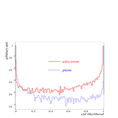
Figure 2: Likelihood ratio. Electrons and pions are denoted by solid broken histograms, respectively.

Figure 2 shows the distribution of $L_{eid}$ using all the discriminants described below. Both electrons and charged pions are shown. As can be seen, significant e/$\pi$ separation is achieved with this variable.

3.2 The Discriminants

We use the following five discriminants in the EID:

1. Matching between the position of the charged track extrapolated to the ECL and the energy cluster position measured by the ECL.

2. Ratio of the energy measured by the ECL, $E$, and the charged track momentum measured by the CDC, $p$.

3. Transverse shower shape at the ECL.

4. $dE/dx$ in the CDC.

5. Light yield in the ACC.

Below we discuss each discriminant in detail. In each case data are used to show the detector performance for electrons and hadrons. For electrons, a sample of radiative Bhabha events are used, while for hadron backgrounds $\mbox{$K_{S}$}\rightarrow\mbox{$\pi^{+}$}\mbox{$\pi^{-}$}$ decays in hadronic events are used. Since the first item, matching between CDC tracks and ECL clusters, is needed to derive the $E/p$ and the shower shape at the ECL, we describe the matching first. We then go through the remaining discriminants: ECL, CDC, and ACC in order.

3.2.1 Position Matching of the ECL Cluster to the Charged Track

The position matching between charged tracks and ECL clusters contributes to the EID in two ways. First, it helps to discriminate between electrons and hadrons directly, since the position resolution for electron showers is considerably smaller than that for hadronic showers. Second, proper position matching is essential to derive the correct ratio for $E/p$, which gives the largest discriminating power between electrons and hadrons.

To obtain reliable matching between the extrapolated track and the center of gravity of the electron’s shower, it is necessary to ensure that the track is extrapolated to the appropriate depth in the calorimeter. This is particularly important at low momenta, where the track curvature can be significant. Thus we use a momentum dependent extrapolation depth, which is derived from Monte Carlo (MC) simulation [5]. The extrapolation direction is determined using the momentum vector of the incident charged particle at the front surface of the ECL.

Defining the difference between the cluster position and the position of an electron track extrapolated to the ECL in $\phi$ (azimuth) as $\Delta\phi$, and in $\theta$ (polar angle) as $\Delta\theta$, we define a matching $\chi^{2}$ as

$$\chi^{2}\equiv\left(\frac{\Delta\phi}{\sigma_{\Delta\phi}}\right)^{2}+\left(\frac{\Delta\theta}{\sigma_{\Delta\theta}}\right)^{2}\;,$$

where $\sigma$ is the width obtained by fitting the $\Delta\phi$ and $\Delta\theta$ distributions for electrons with Gaussian functions. For each charged track, the cluster giving the minimum $\chi^{2}$ is taken for the matched cluster, and is used to calculate $E/p$ and to derive the transverse shower shape. If no cluster with a matching $\chi^{2}$ less than 50 is found, the track is considered to have no associated ECL cluster.

Figure 4 shows $\Delta\phi$ (top) and $\Delta\theta$ (bottom) for electrons and pions. As can be seen, electron clusters exhibit better track matching than the pion clusters do. The position matching $\chi^{2}$ distributions for electrons and pions are shown in Fig. 4. This $\chi^{2}$ distribution is used as one of the discriminants.

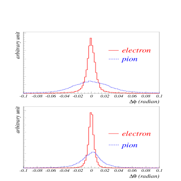
Figure 3: $\Delta\phi$ (top) and $\Delta\theta$ (bottom). The solid (broken) line shows the electron (charged pion) case.

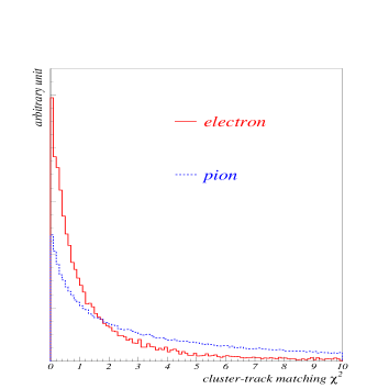
Figure 4: Cluster-track matching $\chi^{2}$. The solid (broken) line shows the electron (charged pion) case.

3.2.2 $E/p$

Since electrons in the energy range of interest have negligible mass, we have $E=\sqrt{p^{2}+m^{2}}\simeq p$ and we expect that the ratio $E/p=1$ within measurement errors. For pions and other hadrons $E/p$ is typically smaller than one, and, more importantly, the energy deposition for hadronic showers is highly variable.

Figure 6 shows $E/p$ distribution for electrons in the momentum region $0.5<p_{\rm lab}<3.0$ GeV/$c$ . Also shown is $E/p$ for charged pions. As can be seen, $E/p$ gives a large discriminating power between electrons and hadrons. For example, a simple cut of $E/p>0.8$ would give the efficiency of 76.1% for electrons, and 3.4% for pions.

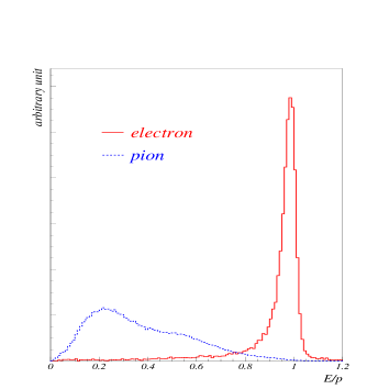
Figure 5: $E/p$ for electrons (solid) and charged pions (broken).

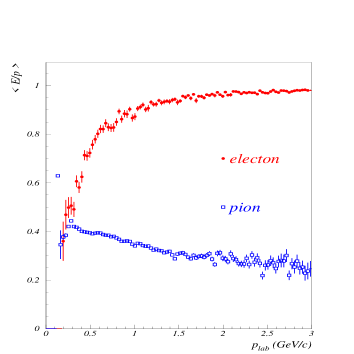
Figure 6: Momentum dependence of $E/p$. Electrons are represented by filled circles, and charged pions by open squares.

The lower-side tail in the electron $E/p$ distribution comes from the interactions of electrons with material in front of the ECL. Figure 6 shows the momentum dependence of $E/p$. The lower the momentum, the larger the fraction of events that have $E/p$ different from unity as a result of interactions. On the other hand, pions have a lower $E/p$ at higher the momenta, so that $E/p$ is an efficient parameter in EID for high momentum particles.

3.2.3 Shower Shape

Electromagnetic and hadronic showers have different shapes in both the transverse and the longitudinal directions. To evaluate the shower shapes in the transverse direction quantitatively, we use the quantity $E9/E25$, which is defined as the ratio of energy summed in a 3 $\times$ 3 array of crystals surrounding the crystal at the center of the shower to that of a sum of a 5 $\times$ 5 array of crystals centered on the same crystal.

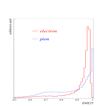
Figure 7: $E9/E25$ for electrons and pions denoted by solid broken histograms, respectively.

Figure 7 shows $E9/E25$ for electrons and charged pions. Electrons exhibit a peak at around $E/p=0.95$, with a relatively small low-side tail, while pions have more events in the lower $E9/E25$ range. This is attributed to the faster evolution (measured in terms of material depth) of electromagnetic showers relative to that for hadronic showers. The events in the region of the pion distribution near unity arise from minimum ionizing energy deposit in a single ECL block.

3.2.4 $dE/dx$

The amount of ionization created by a particle as it travels through a gas filled volume is proportional to its rate of energy loss, $dE/dx$, which exhibits a well-known $\beta^{-2}$ dependence. Although the statistical fluctuations for any single $dE/dx$ measurement are typically quite large, and exhibit a pronounced high-side tail, an accurate determination of $dE/dx$ can be made by averaging several measurements. By excluding the highest 20% of the individual measurements from the average, the effects of upward fluctuations can be suppressed. Figure 9 shows the resulting $dE/dx$ distributions for electrons and for pions. The resolution for pions is 7.8%.

The averaged $dE/dx$ as a function of momentum is shown in Fig. 9.

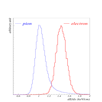
Figure 8: $dE/dx$ for electrons and pions. The solid histogram represents electrons, and the broken histogram represents pions.

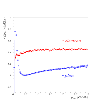
Figure 9: Momentum dependence of $dE/dx$. Electrons are represented by filled circles, and pions by open squares.

As can be seen, the momentum range of interest is almost fully covered by $dE/dx$ in terms of e/$\pi$ separation, although the separating power is higher in the lower momentum region. This approach is complementary to the $E/p$ approach.

The likelihood for $dE/dx$ is calculated from the measured $dE/dx$ ($(dE/dx)_{\rm meas}$), expected $dE/dx$ ($(dE/dx)_{\rm exp}$), and the expected resolution ($\sigma_{dE/dx}$), assuming the PDF to be a Gaussian. The mean of the Gaussian is deduced from the Bethe-Bloch equation as a function of velocity based on an arbitrary particle hypothesis. The expected resolution is determined from test beam results. Given a $\chi^{2}$ of

$$\chi^{2}=(\frac{(dE/dx)_{\rm meas}-(dE/dx)_{\rm exp}}{\sigma_{dE/dx}})^{2}\;,$$

the likelihood probability, $L$, is expressed as

$$L=\frac{e^{-\frac{1}{2}\chi^{2}}}{\sqrt{2\pi}\sigma_{dE/dx}}\;.$$

3.2.5 Light Yield in the ACC

In the ACC, the Cherenkov threshold for electrons is just a few MeV, while that for pions is 0.5 to 1.0 GeV/$c$, depending on the refractive index. Therefore, the ACC is able to distinguish between electrons and hadrons in the momentum region below $\sim 1.0$ GeV/$c$. A likelihood is calculated from the light yield of the aerogel radiator (actually by the number of photoelectrons from the PMT) using PDFs calculated from MC distributions for 20 different velocity ranges.

3.3 PDFs for Discriminants Related to the ECL

PDFs for $E/p$, $E9/E25$, and the position matching $\chi^{2}$ are created in a manner similar to the one described below. Two sets of PDFs are prepared, one for data, and another for MC. For producing electron PDFs in real data analysis, we use real $e^{+}e^{-}\rightarrow e^{+}e^{-}e^{+}e^{-}$ events.

The PDFs for non-electrons are generated using hadronic MC events. This is done for both data PDFs and MC PDFs. The MC sample used for this purpose consists of generic $B-\bar{B}$ decays and continuum events in a 1:3 ratio. Random-trigger events from the experiment are overlaid on the MC events to simulate accidental backgrounds. The shapes of the PDFs are parametrized by fitting the distributions of each discriminant to shape functions selected by trial and error. A summary of the selected shape functions appears in Table 1.

Table 1: Shape of PDFs.

discriminant	function modeling the shape
$E/p$ for $e^{\pm}$	$f(x)=(1-E)\times A\times\exp[-\frac{1}{2}(\frac{x-B}{\sigma})^{2}]$
	$+E\times A\times\exp[-\frac{1}{2}(\frac{x-B}{F})^{2}]$
	where the $\sigma$ is $C+D(x-B)$ if $x<B$, and is $C$ if $x>B$.
$E/p$ for $\pi^{\pm}$	triple Gaussian + linear
$E9/E25$ for $e^{\pm}$	$g(x)=A\times\exp[-\frac{1}{2}(\frac{x-B}{C+D(x-B)})^{2}]$
$E9/E25$ for $\pi^{\pm}$	$h(x)=g(x)$ + Gaussian
matching $\chi^{2}$ for $e^{\pm}$	exponential + linear
matching $\chi^{2}$ for $\pi^{\pm}$	exponential + linear

To take into account the momentum and polar angle dependence of the PDFs, the fits to the PDF functions are carried out in ten momentum bins and six polar angle bins (total of 60 bins in all). The bins are divided into

• 0.0-0.6, 0.6-0.7, 0.7-0.82, 0.82-0.95, 0.95-1.1, 1.1-1.27, 1.27-1.47, 1.47-1.7, 1.7-2.05, and $>$2.05 GeV/$c$ in lab. frame momentum;

• $<33.6^{\circ}$ (forward endcap region), $33.6^{\circ}$ - $45.9^{\circ}$, $45.9^{\circ}$ - $70.6^{\circ}$, $70.6^{\circ}$ - $109.4^{\circ}$, $109.4^{\circ}$ - $132.5^{\circ}$, and $>132.5^{\circ}$ (backward endcap region) in polar angle. The polar angle bins correspond to the boundaries of six different groups of CsI crystals in the ECL.

4 Efficiency

Two different types of event samples are used to study the efficiency of the EID. The first are QED events which provide a clean source of electrons over a wide momentum range. These serve as a good calibration sample. However, to take into account possible efficiency degradations for electrons in hadronic events, where there are more charged tracks, more ECL energy clusters, and more accidental hits in all detectors, we also studied the EID efficiency in a hadronic environment.

We here define EID efficiency as

$$\rm efficiency=\frac{Number\;of\;tracks\;identified\;as\;an\;electron}{Number\;of\;electron\;tracks\;found\;by\;tracking}\;,$$

where the threshold is applied at 0.5 on $L_{\rm eid}$. Note that the tracking efficiency is not included here. Unless otherwise mentioned, the charged tracks used in this study are required to come from the IP. 

4.1 Efficiency in QED Events

The EID efficiency in radiative Bhabha events  is measured and compared with MC expectations as shown in Fig. 11. The polar angle here is restricted to be $-0.57<\cos\theta<0.82$. This eliminates the very forward and very backward regions, where the EID efficiency is difficult to evaluate owing to tracking instabilities brought on by large beam-induced backgrounds. The measured efficiency in the momentum range above 1 GeV/$c$ is over 90% and is in good agreement with MC prediction. This momentum region includes most of the range populated by electrons from $J/\psi\rightarrow e^{+}e^{-}$ decays as well as most of the electrons used in flavor tagging.

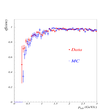
Figure 10: Efficiency in radiative Bhabha events as a function of lab momentum. Data are represented by filled circles, and MC simulation by open squares.

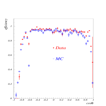
Figure 11: Efficiency in radiative Bhabha events as a function of $\cos\theta$ of a track. Data are represented by filled circles, and MC simulation by open squares.

The polar angle dependence of the efficiency is shown in Fig. 11. The momentum range of the electrons is $0.5<p_{\rm lab}<2.5$ GeV/$c$. Although the agreement between data and MC is good, the efficiency itself in the endcap region is much lower than that in the barrel. This is because more material exists in the endcap region, which degrades both the ECL’s resolution and the CDC’s tracking performance. The low efficiency seen at $\cos\theta\sim-0.6$ is due to a gap between the barrel part and endcap part of the ECL.

4.2 Efficiency in Hadronic Events

The EID efficiency in hadronic events is studied using 1) single-electron MC tracks embedded in real hadronic events, and 2) $J/\psi(\rightarrow e^{+}e^{-})$ inclusive events.

4.2.1 Single $e^{\pm}$ MC Embedded in Hadronic Events

A comparison between the efficiency obtained for isolated single-track electrons and for electron tracks embedded in hadronic data events is shown in Table 2. Since the polar angle distributions for the hadronic MC and the single electron MC tracks are different, only the $-0.57<\cos\theta<0.82$ region is used for this comparison.

Table 2: Efficiency (%) in the region of $-0.57<\cos\theta<0.82$.

$p_{\rm lab}$(GeV)	single MC	single MC in hadronic events	generic hadronic MC
0.00-0.25	$41.0\pm 5.4$	$42.0\pm 5.9$	$51.5\pm 1.2$
0.25-0.50	$72.1\pm 1.2$	$68.2\pm 1.4$	$71.0\pm 1.0$
0.50-0.75	$83.5\pm 0.9$	$81.7\pm 1.0$	$82.4\pm 0.9$
0.75-1.00	$91.2\pm 0.7$	$89.2\pm 0.8$	$90.4\pm 0.8$
1.00-1.25	$94.4\pm 0.6$	$90.8\pm 0.7$	$93.0\pm 0.8$
1.25-1.50	$96.4\pm 0.5$	$93.4\pm 0.6$	$95.1\pm 0.8$
1.50-1.75	$98.0\pm 0.4$	$94.8\pm 0.6$	$96.0\pm 0.8$
1.75-2.00	$97.5\pm 0.4$	$96.2\pm 0.5$	$95.5\pm 1.0$
2.00-2.25	$98.1\pm 0.3$	$95.8\pm 0.5$	$96.7\pm 1.1$
2.25-2.50	$98.7\pm 0.3$	$95.7\pm 0.6$	$95.3\pm 1.9$

The efficiency for MC-generated single-track electrons having momenta greater than 0.5 GeV/$c$ drops by 2.5% when these tracks are embedded into hadronic events from the data sample. This degradation is significant for the $dE/dx$ and the cluster-track matching efficiencies. No statistically significant degradation is seen in $E/p$ or $E9/E25$. The good agreement between the single-track MC electrons embedded in hadronic events and the generic hadronic MC implies that the efficiency drop due to the hadronic environment is well reproduced in our generic-hadron MC. We will therefore refer to the efficiency estimated by the generic hadronic MC as the EID efficiency since the momentum and angular distributions imitate hadronic data. This reference efficiency is shown in Fig. 12. For momentum region $1.0~{}(0.5)<p_{\rm lab}<3.0$ GeV/$c$ and for the whole polar angle range, the efficiency is $(92.4\pm 0.4)\%$ ($(87.3\pm 0.3)\%$).

Figure 12: Efficiency in the generic hadronic MC. The left plot shows the momentum dependence of the EID efficiency. The efficiency for $-0.57<\cos\theta<0.82$ is illustrated by filled circles, and that for the full region by open squares. The right plot shows the polar angle dependence for the momentum greater than 0.5 GeV/$c$ in the lab frame.

One note here is that there is a strong correlation between lab frame momentum and polar angle because of the asymmetric beam energy. For example the forward endcap region seems to have higher efficiency than that of barrel from Fig. 12, however, this effect is caused by the harder momentum spectrum in the forward region. The barrel region has higher efficiency for the same momentum.

In the next subsections, we further examine the efficiency in hadronic events by comparing data and MC.

4.2.2 $J/\psi(\rightarrow e^{+}e^{-})$ Inclusive Events

One can also obtain the EID efficiency or inefficiency by comparing the $J/\psi(\rightarrow e^{+}e^{-})X$ yield for the cases one or two electrons are tagged, or the difference of the two cases. To estimate the signal yield, we use the $M_{ee}$ distribution as shown in Fig. 13.

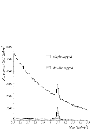
Figure 13: $M_{ee}$ distributions. The open (hatched) histogram shows $M_{ee}$ with one (both) track(s) identified as an electron.

The sample is selected using the standard hadronic event selection in Belle:

• The number of good tracks is required to be $\geq 3$, where a good track is defined to be one with $|dr|<2.0$ cm, $|dz|<4.0$ cm, and $p_{t}>0.1$ GeV/$c$.

• The primary vertex position has to be $<1.5$ cm in radius and within $\pm 3.5$ cm of the IP in $z$.

• The sum of charged-track momentum and ECL cluster energy in the $\Upsilon(4S)$ rest frame is $\geq 20\%$ of the center-of-mass energy ($\equiv W$).

• $|\sum p_{z}^{*}|<50\%$ of $W$, where $p_{z}^{*}$ is $z$ component of momentum for either charged tracks or ECL cluster energies in the center-of-mass frame.

• The sum of ECL cluster energies is between 2.5% and 90% of $W$.

In addition the ratio of the 2nd Fox-Wolfram moment [6] to the 0th moment, R2, is required to be below 0.5 to suppress continuum events. Because there are many QED related backgrounds such as radiative Bhabha events in which the photon is converted to an $e^{+}e^{-}$ pair, we require that the selected events have at least one electron in the barrel region and we raise the good-track requirement to $\geq 5$. A requirement of $L_{eid}>0.5$ is used for tagging. The electron momentum spectrum for the surviving events turns on at around 0.7 GeV/$c$ and extends up to $\sim 3.5$ GeV/$c$ with a peak at about 1.6 GeV/$c$ in the laboratory frame.

To model the signal shape, we first fit the distribution of double tagged $M_{ee}$ events with a “crystal-ball function”  for the signal and exponential for the background. The same procedure is carried out for the sample of single-tagged events, and that of single-tagged events subtracted by double-tagged events. In the fitting of these $M_{ee}$ spectra, the signal peak position and width are fixed to the values extracted from the double-tagged $M_{ee}$ spectrum, with only the signal yield being allowed to float freely.

Using the procedure above, the signal yield for the mass range between 2.5 and 3.5 GeV/$c^{2}$ is estimated to be $4107.9\pm 112.0$ for single tagging, and $540.2\pm 131.6$ for the difference between single and double tagged events. Since the signal yield with single tagging (difference between single tagging and double tagging) is proportional to $1-\bar{\epsilon}^{2}$ ($2\bar{\epsilon}(1-\bar{\epsilon}$)), where the $\bar{\epsilon}$ denotes inefficiency, an inefficiency $(6.2\pm 1.4)\%$ is deduced. This is consistent with the inefficiency of $(5.6\pm 0.1)\%$ that is predicted by the MC.

4.3 Charge Dependence

Since a charge asymmetry in the efficiency would cause a bias in the flavor tagging of initial $B$ states, it is important to examine this possibility closely. To obtain good statistics we used a sample of $e^{+}e^{-}\rightarrow e^{+}e^{-}e^{+}e^{-}$ events. Owing to the asymmetric beam energies, the polar angular distributions of electrons and positrons differ, so the efficiencies were compared for individual bins in momentum and angle. Figure 14 shows the efficiency for the $e^{+}e^{-}\rightarrow e^{+}e^{-}e^{+}e^{-}$ sample divided into six different polar angle regions as a function of laboratory momentum. The polar-angle division corresponds to the six groups of PDFs described in Section 3.3. The efficiencies for electrons and positrons are separately illustrated.

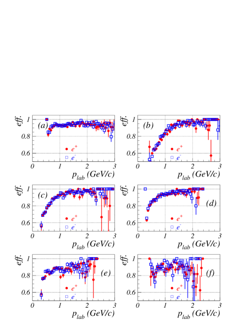
Figure 14: Efficiency in $e^{+}e^{-}\rightarrow e^{+}e^{-}e^{+}e^{-}$ events as a function of momentum in lab. frame. The efficiency for positrons is denoted by filled circles, and that for electrons by open squares. Each plot corresponds to a different polar angle. The (a) is for the forward endcap, (b) through (e) for the barrel, and (f) for the backward endcap. The division is the same as in the PDFs for likelihood using $E/p$ etc..

No statistically significant difference in efficiency for the barrel region between electrons and positrons is observed. For the endcap region, the charge dependence still exists even with this polar-angle division because of the different angular-momentum correlation between electrons and positrons. From these data one can extract 90% confidence interval of $-0.002<A_{chg}<0.002$ on the charge asymmetry for the momentum range between 0.5 GeV/$c$ and 2.5 GeV/$c$ in the barrel region.

5 Fake rate

In addition to the efficiency, the fake rate is another important factor in EID performance. We define the fake rate as:

$$\rm fake\;rate=\frac{\#\;of\;non\;e^{\pm}\;tracks\;found\;by\;tracking\;with\;the\;{\it L}_{eid}>0.5}{\#\;of\;non\;e^{\pm}\;tracks\;found\;by\;tracking}$$

In this section, we discuss the fake rate for $\pi^{\pm}$. The comparison between data and MC, and the charge dependence are described. We also mention the measurement of fake rate for $K^{\pm}$.

5.1 Fake rate to $\pi^{\pm}$

We use inclusive $\mbox{$K_{S}$}\rightarrow\pi^{+}\pi^{-}$ decays as a source of charged pions to measure the EID fake rate. The $\mbox{$K_{S}$}\rightarrow\pi^{+}\pi^{-}$ decays are selected from two oppositely charged tracks with the following selection criteria:

• The Belle standard hadronic event selection.

• The distance in $z$ between the two helices at the decay vertex has to be less than 1 cm.

• The deflection angle, defined as the angle between the $K_{S}$ momentum vector and the vector extrapolated from the IP to the $K_{S}$ decay vertex, must be less than $15^{\circ}$.

• The impact parameter in the $x$-$y$ view is required to be greater than 1 mm.

• The invariant mass reconstructed from the two pion tracks, $M_{\mbox{$\pi^{+}$}\mbox{$\pi^{-}$}}$, satisfies $487.7<M_{\mbox{$\pi^{+}$}\mbox{$\pi^{-}$}}<507.7$ MeV/$c^{2}$.

• One track of the pair is identified as a charged pion by requiring $L_{eid}<0.01$ and vetoing protons using another particle identification package for hadrons in Belle [4]. (No requirement is placed on the pion used to test the EID routines.)

Figure 16 shows the fake rate as a function of laboratory momentum with a plot of the MC expectation superimposed. Data and MC agree well for momenta above 0.5 GeV/$c$.

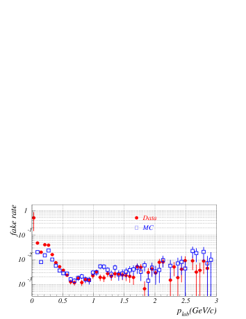
Figure 15: Fake rate for $\pi^{\pm}$ as a function of momentum. The data are shown as filled circles, and the MC as open squares.

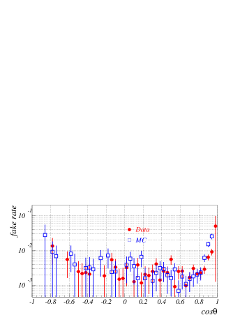
Figure 16: Fake rate for $\pi^{\pm}$ as a function of polar angle. The data are shown as filled circles, and the MC as open squares.

The result obtained from this sample is also summarized in Table 3.

The polar angle dependence is shown in Fig. 16. The overall agreement between data and MC is good, although the fake rate in the data is slightly lower than MC expectation. For example, the fake rate in the momentum range between 0.5 and 3.0 GeV/$c$ is $(0.22\pm 0.01)\%$ in data, and $(0.27\pm 0.01)\%$ in MC. This disagreement mainly comes from an inconsistency in the forward endcap region. If the polar angle is restricted to the barrel region only ($-0.57<\cos\theta<0.82$) the fake rates are $(0.16\pm 0.01)\%$ for both data and MC.

Table 3: Fake rate (%) to charged pions in real data.

$p_{\rm lab}$(GeV)	$\pi^{\pm}$	$\pi^{+}$	$\pi^{-}$
0.00-0.25	$3.50\pm 0.09$	$3.57\pm 0.13$	$3.43\pm 0.13$
0.25-0.50	$1.51\pm 0.04$	$1.50\pm 0.05$	$1.52\pm 0.05$
0.50-0.75	$0.20\pm 0.02$	$0.24\pm 0.03$	$0.16\pm 0.02$
0.75-1.00	$0.15\pm 0.02$	$0.19\pm 0.03$	$0.12\pm 0.02$
1.00-1.25	$0.25\pm 0.03$	$0.26\pm 0.04$	$0.24\pm 0.04$
1.25-1.50	$0.25\pm 0.04$	$0.30\pm 0.06$	$0.21\pm 0.05$
1.50-1.75	$0.29\pm 0.06$	$0.35\pm 0.09$	$0.24\pm 0.07$
1.75-2.00	$0.31\pm 0.07$	$0.46\pm 0.13$	$0.17\pm 0.08$
2.00-2.25	$0.42\pm 0.11$	$0.28\pm 0.12$	$0.57\pm 0.18$
2.25-2.50	$0.45\pm 0.14$	$0.18\pm 0.12$	$0.73\pm 0.26$
2.50-2.75	$0.42\pm 0.17$	$0.42\pm 0.24$	$0.43\pm 0.25$
2.75-3.00	$0.32\pm 0.19$	$0.00\pm 0.00$	$0.68\pm 0.39$

5.2 Charge Dependence in Fake Rate

The charge dependence of the fake rate is also checked using $\mbox{$K_{S}$}\rightarrow\pi^{+}\pi^{-}$ events. The fake rates for $\pi^{+}$ and $\pi^{-}$ are separately listed in Table 3. As the table shows, the fake rate for $\pi^{+}$ is systematically higher than that for $\pi^{-}$ for momentum below 2 GeV/$c$. On the other hand, the fake rate for $\pi^{+}$ is lower than that for $\pi^{-}$ above 2 GeV/$c$. This is due to the different nuclear shower evolution between $\pi^{+}$ and $\pi^{-}$, resulting in non-identical $E/p$ distributions.

5.3 Fake Rate to $K^{\pm}$

The fake rate for $K^{\pm}$ is examined using the decay chain $D^{*+}\rightarrow D^{0}(\rightarrow K^{-}\pi^{+})\pi^{+}_{s}$, where the subscript of $\pi^{+}_{s}$ is used as a flag to signify that the $\pi^{+}$ comes from $D^{*+}$ decay or $D^{0}$ decay. This decay chain allows us to have a $K^{-}$ sample without any particle identification because the charge of $\pi_{s}$ serves as a discriminant between $K^{-}$ and $\pi^{+}$ through its charge correlation.

The strategy for evaluating the fake rate is to compare the signal yield of $D^{0}$ with and without applying EID for the kaons. The $D^{0}$ signal yield is measured by fitting the mass distribution to the sum of a Gaussian for the signal and a linear function for the background. The selection criteria for the $D^{*}$ decay chain are:

• Defining $\theta$ as the angle between the $K^{-}$ flight direction in the $D^{0}$ rest frame and the $D^{0}$ flight direction in the $\Upsilon(4S)$ frame, $|\cos\theta|<0.8$.

• Defining $x$ as the $D^{*+}$ momentum in the $\Upsilon(4S)$ rest frame divided by the beam energy in that frame, $x$ is required to be $>0.45$. This allows us to select continuum events, simplifying comparison between data and MC.

• The reconstructed mass difference between the $D^{*+}$ and the $D^{0}$ is within 1.5 MeV/$c^{2}$ from the nominal mass difference.

After the above selection, we have 16470$\pm$150.0 events without EID, and 71.4$\pm$18.5 events after applying EID. Taking the ratio, the fake rate for the kaons is measured to be $(0.43\pm 0.07)\%$ This can be compared to the MC prediction of $(0.21\pm 0.05)\%$ for the fake rate.

6 Conclusions

Using a generic hadronic MC sample consisting of $B-\bar{B}$ and continuum events in a 1:3 ratio with randomly triggered events overlaid, the EID efficiency is estimated to be $(92.4\pm 0.4)\%$ for the momentum range $1.0<p_{\rm lab}<3.0$ GeV/$c$. Using inclusive $K_{S}\rightarrow\mbox{$\pi^{+}$}\mbox{$\pi^{-}$}$ events, the fake rate to charged pions is measured to be $(0.25\pm 0.02)\%$ for $1.0<p_{\rm lab}<3.0$ GeV/$c$.

The EID efficiency expected from the generic hadronic MC is consistent with that for single electrons in real hadronic data within 1%. Using $J/\psi\rightarrow e^{+}e^{-}$ events, the EID inefficiency is verified to be consistent between data and MC within a 1.4% uncertainty. The fake rate measured in data is consistent with the MC expectation to 0.05% in absolute value. For a restricted theta range ($-0.57<\cos\theta<0.82$), the fake rate in data agrees with MC expectations within 0.01%.

References

-
[1]
Belle Collaboration,
Phys. Rev. Lett. 86, 2509.
Belle Collaboration, Phys. Rev. Lett. 87, 091802. - [2] I.I. Bigi and A.I. Sanda. “CP Violation”, Cambridge Univ. Press.
- [3] J.W. Nam, “Results on Inclusive and Semileptonic Decays from Belle.”, Proceedings DPF 2000.
- [4] Belle Collaboration, KEK Preprint 2000-4.
- [5] GEANT Detector Description and Simulation Tool, CERN Program Library Long Writeup W5013.
- [6] G.C. Fox and S. Wolfram, Phys. Rev. Lett. 41, 1581 (1978).
- [7] Particle Data Group, Euro. Phys. J. C15, 1 (2000).