EUROPEAN ORGANIZATION FOR NUCLEAR RESEARCH

CERN-EP-2001-058

31 July 2001

Measurement of the Branching Ratio for the Process ${{\rm b}\to\tau^{-}\overline{\nu}_{\tau}{\rm X}}$

The OPAL Collaboration

Abstract

The inclusive branching ratio for the process ${\rm b}\to\tau^{-}\overline{\nu}_{\tau}{\rm X}$ has been measured using hadronic ${\rm Z}$ decays collected by the OPAL experiment at LEP in the years 1992-2000. The result is:

$$\mathrm{BR}({{\rm b}\to\tau^{-}\overline{\nu}_{\tau}{\rm X}})=(2.78\pm 0.18\pm 0.51)\%$$

This measurement is consistent with the Standard Model expectation and puts a constraint of

$$\tan\beta/M_{\rm H}^{\pm}<0.53\ {\rm GeV}^{-1}$$

at the $95\%$ confidence level on Type II Two Higgs Doublet Models.

(Submitted to Physics Letters B)

The OPAL Collaboration

G. Abbiendi², C. Ainsley⁵, P.F. Åkesson³, G. Alexander²², J. Allison¹⁶, G. Anagnostou¹, K.J. Anderson⁹, S. Arcelli¹⁷, S. Asai²³, D. Axen²⁷, G. Azuelos^18,a, I. Bailey²⁶, E. Barberio⁸, R.J. Barlow¹⁶, R.J. Batley⁵, T. Behnke²⁵, K.W. Bell²⁰, P.J. Bell¹, G. Bella²², A. Bellerive⁹, S. Bethke³², O. Biebel³², I.J. Bloodworth¹, O. Boeriu¹⁰, P. Bock¹¹, J. Böhme²⁵, D. Bonacorsi², M. Boutemeur³¹, S. Braibant⁸, L. Brigliadori², R.M. Brown²⁰, H.J. Burckhart⁸, J. Cammin³, R.K. Carnegie⁶, B. Caron²⁸, A.A. Carter¹³, J.R. Carter⁵, C.Y. Chang¹⁷, D.G. Charlton^1,b, P.E.L. Clarke¹⁵, E. Clay¹⁵, I. Cohen²², J. Couchman¹⁵, A. Csilling^8,i, M. Cuffiani², S. Dado²¹, G.M. Dallavalle², S. Dallison¹⁶, A. De Roeck⁸, E.A. De Wolf⁸, P. Dervan¹⁵, K. Desch²⁵, B. Dienes³⁰, M.S. Dixit^6,a, M. Donkers⁶, J. Dubbert³¹, E. Duchovni²⁴, G. Duckeck³¹, I.P. Duerdoth¹⁶, E. Etzion²², F. Fabbri², L. Feld¹⁰, P. Ferrari¹², F. Fiedler⁸, I. Fleck¹⁰, M. Ford⁵, A. Frey⁸, A. Fürtjes⁸, D.I. Futyan¹⁶, P. Gagnon¹², J.W. Gary⁴, G. Gaycken²⁵, C. Geich-Gimbel³, G. Giacomelli², P. Giacomelli², D. Glenzinski⁹, J. Goldberg²¹, K. Graham²⁶, E. Gross²⁴, J. Grunhaus²², M. Gruwé⁸, P.O. Günther³, A. Gupta⁹, C. Hajdu²⁹, M. Hamann²⁵, G.G. Hanson¹², K. Harder²⁵, A. Harel²¹, M. Harin-Dirac⁴, M. Hauschild⁸, J. Hauschildt²⁵, C.M. Hawkes¹, R. Hawkings⁸, R.J. Hemingway⁶, C. Hensel²⁵, G. Herten¹⁰, R.D. Heuer²⁵, J.C. Hill⁵, K. Hoffman⁹, R.J. Homer¹, D. Horváth^29,c, K.R. Hossain²⁸, R. Howard²⁷, P. Hüntemeyer²⁵, P. Igo-Kemenes¹¹, K. Ishii²³, A. Jawahery¹⁷, H. Jeremie¹⁸, C.R. Jones⁵, P. Jovanovic¹, T.R. Junk⁶, N. Kanaya²⁶, J. Kanzaki²³, G. Karapetian¹⁸, D. Karlen⁶, V. Kartvelishvili¹⁶, K. Kawagoe²³, T. Kawamoto²³, R.K. Keeler²⁶, R.G. Kellogg¹⁷, B.W. Kennedy²⁰, D.H. Kim¹⁹, K. Klein¹¹, A. Klier²⁴, S. Kluth³², T. Kobayashi²³, M. Kobel³, T.P. Kokott³, S. Komamiya²³, R.V. Kowalewski²⁶, T. Krämer²⁵, T. Kress⁴, P. Krieger⁶, J. von Krogh¹¹, D. Krop¹², T. Kuhl³, M. Kupper²⁴, P. Kyberd¹³, G.D. Lafferty¹⁶, H. Landsman²¹, D. Lanske¹⁴, I. Lawson²⁶, J.G. Layter⁴, A. Leins³¹, D. Lellouch²⁴, J. Letts¹², L. Levinson²⁴, J. Lillich¹⁰, C. Littlewood⁵, S.L. Lloyd¹³, F.K. Loebinger¹⁶, G.D. Long²⁶, M.J. Losty^6,a, J. Lu²⁷, J. Ludwig¹⁰, A. Macchiolo¹⁸, A. Macpherson^28,l, W. Mader³, S. Marcellini², T.E. Marchant¹⁶, A.J. Martin¹³, J.P. Martin¹⁸, G. Martinez¹⁷, G. Masetti², T. Mashimo²³, P. Mättig²⁴, W.J. McDonald²⁸, J. McKenna²⁷, T.J. McMahon¹, R.A. McPherson²⁶, F. Meijers⁸, P. Mendez-Lorenzo³¹, W. Menges²⁵, F.S. Merritt⁹, H. Mes^6,a, A. Michelini², S. Mihara²³, G. Mikenberg²⁴, D.J. Miller¹⁵, S. Moed²¹, W. Mohr¹⁰, T. Mori²³, A. Mutter¹⁰, K. Nagai¹³, I. Nakamura²³, H.A. Neal³³, R. Nisius⁸, S.W. O’Neale¹, A. Oh⁸, A. Okpara¹¹, M.J. Oreglia⁹, S. Orito²³, C. Pahl³², G. Pásztor^8,i, J.R. Pater¹⁶, G.N. Patrick²⁰, J.E. Pilcher⁹, J. Pinfold²⁸, D.E. Plane⁸, B. Poli², J. Polok⁸, O. Pooth⁸, A. Quadt³, K. Rabbertz⁸, C. Rembser⁸, P. Renkel²⁴, H. Rick⁴, N. Rodning²⁸, J.M. Roney²⁶, S. Rosati³, K. Roscoe¹⁶, Y. Rozen²¹, K. Runge¹⁰, D.R. Rust¹², K. Sachs⁶, T. Saeki²³, O. Sahr³¹, E.K.G. Sarkisyan^8,m, C. Sbarra²⁶, A.D. Schaile³¹, O. Schaile³¹, P. Scharff-Hansen⁸, C. Schmitt¹⁰, M. Schröder⁸, M. Schumacher²⁵, C. Schwick⁸, W.G. Scott²⁰, R. Seuster^14,g, T.G. Shears^8,j, B.C. Shen⁴, C.H. Shepherd-Themistocleous⁵, P. Sherwood¹⁵, A. Skuja¹⁷, A.M. Smith⁸, G.A. Snow¹⁷, R. Sobie²⁶, S. Söldner-Rembold^10,e, S. Spagnolo²⁰, F. Spano⁹, M. Sproston²⁰, A. Stahl³, K. Stephens¹⁶, D. Strom¹⁹, R. Ströhmer³¹, L. Stumpf²⁶, B. Surrow²⁵, S. Tarem²¹, M. Tasevsky⁸, R.J. Taylor¹⁵, R. Teuscher⁹, J. Thomas¹⁵, M.A. Thomson⁵, E. Torrence¹⁹, D. Toya²³, T. Trefzger³¹, A. Tricoli², I. Trigger⁸, Z. Trócsányi^30,f, E. Tsur²², M.F. Turner-Watson¹, I. Ueda²³, B. Ujvári^30,f, B. Vachon²⁶, C.F. Vollmer³¹, P. Vannerem¹⁰, M. Verzocchi¹⁷, H. Voss⁸, J. Vossebeld⁸, D. Waller⁶, C.P. Ward⁵, D.R. Ward⁵, P.M. Watkins¹, A.T. Watson¹, N.K. Watson¹, P.S. Wells⁸, T. Wengler⁸, N. Wermes³, D. Wetterling¹¹ G.W. Wilson¹⁶, J.A. Wilson¹, T.R. Wyatt¹⁶, S. Yamashita²³, V. Zacek¹⁸, D. Zer-Zion^8,k

¹School of Physics and Astronomy, University of Birmingham, Birmingham B15 2TT, UK
²Dipartimento di Fisica dell’ Università di Bologna and INFN, I-40126 Bologna, Italy
³Physikalisches Institut, Universität Bonn, D-53115 Bonn, Germany
⁴Department of Physics, University of California, Riverside CA 92521, USA
⁵Cavendish Laboratory, Cambridge CB3 0HE, UK
⁶Ottawa-Carleton Institute for Physics, Department of Physics, Carleton University, Ottawa, Ontario K1S 5B6, Canada
⁸CERN, European Organisation for Nuclear Research, CH-1211 Geneva 23, Switzerland
⁹Enrico Fermi Institute and Department of Physics, University of Chicago, Chicago IL 60637, USA
¹⁰Fakultät für Physik, Albert Ludwigs Universität, D-79104 Freiburg, Germany
¹¹Physikalisches Institut, Universität Heidelberg, D-69120 Heidelberg, Germany
¹²Indiana University, Department of Physics, Swain Hall West 117, Bloomington IN 47405, USA
¹³Queen Mary and Westfield College, University of London, London E1 4NS, UK
¹⁴Technische Hochschule Aachen, III Physikalisches Institut, Sommerfeldstrasse 26-28, D-52056 Aachen, Germany
¹⁵University College London, London WC1E 6BT, UK
¹⁶Department of Physics, Schuster Laboratory, The University, Manchester M13 9PL, UK
¹⁷Department of Physics, University of Maryland, College Park, MD 20742, USA
¹⁸Laboratoire de Physique Nucléaire, Université de Montréal, Montréal, Quebec H3C 3J7, Canada
¹⁹University of Oregon, Department of Physics, Eugene OR 97403, USA
²⁰CLRC Rutherford Appleton Laboratory, Chilton, Didcot, Oxfordshire OX11 0QX, UK
²¹Department of Physics, Technion-Israel Institute of Technology, Haifa 32000, Israel
²²Department of Physics and Astronomy, Tel Aviv University, Tel Aviv 69978, Israel
²³International Centre for Elementary Particle Physics and Department of Physics, University of Tokyo, Tokyo 113-0033, and Kobe University, Kobe 657-8501, Japan
²⁴Particle Physics Department, Weizmann Institute of Science, Rehovot 76100, Israel
²⁵Universität Hamburg/DESY, II Institut für Experimental Physik, Notkestrasse 85, D-22607 Hamburg, Germany
²⁶University of Victoria, Department of Physics, P O Box 3055, Victoria BC V8W 3P6, Canada
²⁷University of British Columbia, Department of Physics, Vancouver BC V6T 1Z1, Canada
²⁸University of Alberta, Department of Physics, Edmonton AB T6G 2J1, Canada
²⁹Research Institute for Particle and Nuclear Physics, H-1525 Budapest, P O Box 49, Hungary
³⁰Institute of Nuclear Research, H-4001 Debrecen, P O Box 51, Hungary
³¹Ludwigs-Maximilians-Universität München, Sektion Physik, Am Coulombwall 1, D-85748 Garching, Germany
³²Max-Planck-Institute für Physik, Föhring Ring 6, 80805 München, Germany
³³Yale University,Department of Physics,New Haven, CT 06520, USA

^a and at TRIUMF, Vancouver, Canada V6T 2A3
^b and Royal Society University Research Fellow
^c and Institute of Nuclear Research, Debrecen, Hungary
^e and Heisenberg Fellow
^f and Department of Experimental Physics, Lajos Kossuth University, Debrecen, Hungary
^g and MPI München
ⁱ and Research Institute for Particle and Nuclear Physics, Budapest, Hungary
^j now at University of Liverpool, Dept of Physics, Liverpool L69 3BX, UK
^k and University of California, Riverside, High Energy Physics Group, CA 92521, USA
^l and CERN, EP Div, 1211 Geneva 23
^m and Tel Aviv University, School of Physics and Astronomy, Tel Aviv 69978, Israel.

1 Introduction

This paper describes a measurement of the inclusive branching ratio BR(${\rm b}\to\tau^{-}\overline{\nu}_{\tau}{\rm X}$ ), using data taken with the OPAL detector at LEP in the years 1992-2000 at e⁺e^- centre-of-mass energies around the Z resonance. Similar measurements of BR(${\rm b}\to\tau^{-}\overline{\nu}_{\tau}{\rm X}$ ) have been published previously by the other LEP experiments [1-3]. The measurements can be directly compared to the Standard Model expectation calculated in the framework of Heavy Quark Effective Theory (HQET) [4], and so can be used to constrain basic parameters of HQET [5].

A measurement of BR(${{\rm b}\to\tau^{-}\overline{\nu}_{\tau}{\rm X}}$) is also a probe for the presence of a new charged boson coupling to mass. This coupling would increase the branching ratio BR(${{\rm b}\to\tau^{-}\overline{\nu}_{\tau}{\rm X}}$) [6, 7]. Since a charged Higgs boson contributes at tree level, its contribution cannot be easily cancelled by other new particles. This can be used to set a limit on a contribution of the charged Higgs exchange. In the Minimal Supersymmetric Standard Model (MSSM), however, a region of the parameter space is found where one-loop SUSY-QCD corrections could weaken the bound [8].

Many extensions of the Standard Model, like the MSSM, include Type II Two Higgs Doublets, where one of two Higgs doublets couples only to down-type quarks and the other only to up-type quarks. In these models, $\tan\beta$ is the ratio of the vacuum expectation values of the two Higgs doublets and $M_{\rm H}^{\pm}$ is the mass of the charged Higgs boson. The decay rate for ${\rm b}\to\tau^{-}\overline{\nu}_{\tau}{\rm X}$  can be calculated as a function of $r=\tan\beta/M_{\rm H}^{\pm}$. A term proportional to $r^{2}$ is added to the Standard Model decay rate of ${\rm BR}({{\rm b}\to\tau^{-}\overline{\nu}_{\tau}{\rm X}})=(2.36\pm 0.17)\%$. A value of $r=0.5$ GeV^-1, for example, yields BR(${{\rm b}\to\tau^{-}\overline{\nu}_{\tau}{\rm X}})=(3.61\pm 0.36)\%$ [7]. The errors are fully correlated and include the experimental uncertainty on ${\rm BR}({{\rm b}\to e^{-}\overline{\nu}_{\rm e}{\rm X}})=(10.86\pm 0.35)\%$ [9] and the theoretical uncertainties.

Since direct reconstruction of the $\tau$ lepton in a multihadronic event is not possible, other properties of the signal decays have to be exploited. Each event is divided into two hemispheres. Hemispheres containing ${\rm b}\to\tau^{-}\overline{\nu}_{\tau}{\rm X}$ decays are characterised by large missing energy, due to the presence of at least two neutrinos in the final state. The reconstruction of the missing energy uses the OPAL calorimeters and tracking detectors and it relies on the hermeticity of the detector. To select a sample enriched in b decays, a b tagging algorithm is applied. The b tagging is done in the hemisphere opposite to the signal to reduce the dependence on the Monte Carlo simulation of the signal.

Semileptonic b decays like b $\rightarrow\ell^{-}\overline{\nu}{\rm X}$ ($\ell={\rm e},\mu$) are an important background. They are suppressed by rejecting hemispheres with an identified electron or muon. The same lepton veto suppresses the leptonic decays of the $\tau$ lepton in signal events, thus selecting mostly hadronic $\tau$ decays.

2 Detector, data set and Monte Carlo samples

The details of the construction and performance of the OPAL detector are described elsewhere [10]. Here only the main components relevant for this analysis are described.

Tracking of charged particles is performed by a central detector, consisting of a silicon microvertex detector, a vertex chamber, a jet chamber and $z$-chambers . The central detector is inside a solenoid, which provides a uniform axial magnetic field of 0.435 T. The silicon microvertex detector consists of two layers of silicon strip detectors; for most of the data used in this paper, the inner layer covered a polar angle range of $|\cos\theta|<0.83$ and the outer layer covered $|\cos\theta|<0.77$, with an extended coverage for the data taken after the year 1996. The vertex chamber is a precision drift chamber which covers the range $|\cos\theta|<0.95$. The jet chamber is a large-volume drift chamber, 4.0 m long and 3.7 m in diameter, providing both tracking and ionisation energy loss (d$E$/d$x$) information. The $z$-chambers provide a precise measurement of the $z$-coordinate of tracks as they leave the jet chamber in the range $|\cos\theta|<0.72$.

Immediately outside the tracking volume is the solenoid and a time-of-flight counter array followed by an electromagnetic shower presampler and a lead-glass electromagnetic calorimeter. The return yoke of the magnet lies outside the electromagnetic calorimeter and is instrumented with limited streamer chambers. It is used as a hadron calorimeter and assists in the reconstruction of muons. The outermost part of the detector is made up by layers of muon chambers.

Hadronic Z decays collected with the OPAL detector at e⁺e^- centre-of-mass energies around the Z resonance are selected using a standard multihadron selection [11]. To reduce further the small contribution of ${\rm Z}\rightarrow\tau^{+}\tau^{-}$ decays an additional requirement of at least 7 tracks in each event is imposed. With these criteria, the selection efficiency for hadronic Z decays is $(98.1\pm 0.5)\%$ [12] with a background of $(0.11\pm 0.03)$%. After hadronic event selection and ${\rm Z}\rightarrow\tau^{+}\tau^{-}$ rejection, the resulting data sample collected in the years 1992-2000 after the installation of the silicon microvertex detector consists of 3.70$\times 10^{6}$ events. About $11\%$ of the data used were recorded in the years 1996-2000, for calibration purposes.

A Monte Carlo sample of hadronic Z decays of about seven times the size of the recorded data sample for b flavour events and about the same size as the recorded data for the other flavours is used in the analysis. The Monte Carlo events are generated using JETSET 7.4 [13] with the b and c quark fragmentation modelled according to the parameterisation of Peterson et al. [14]. A global fit to OPAL data has been performed to optimise the JETSET parameters [15]. The decay ${\rm b}\to\tau^{-}\overline{\nu}_{\tau}{\rm X}$ is modelled in JETSET using matrix elements neglecting the mass of the final state particles. The energy distribution of the $\tau$ lepton in the b rest frame is therefore reweighted to reproduce the energy distribution calculated by including mass effects [4, 16]. The polarisation of the $\tau$ leptons is simulated by interfacing JETSET to the TAUOLA [17] $\tau$ decay simulation package. The $\tau$ polarisation is calculated according to [4] with the HQET parameters $\lambda_{1}$ and $\lambda_{2}$ set to zero, corresponding to the free quark model.

All events have been processed using a full simulation of the OPAL detector [18] and the same reconstruction algorithms that were applied to the data.

3 Event and hemisphere selection

Each event is divided into two hemispheres using the thrust variable, $T$, which is defined by [19]

$$T=\max_{\vec{n}}\left(\frac{\sum_{i}|\vec{p}_{i}\cdot\vec{n}|}{\sum_{i}|\vec{p}_{i}|}\right),$$ (1)

where $\vec{p}_{i}$ are the momentum vectors of the particles in an event. The thrust axis $\vec{n}_{T}$ is the direction $\vec{n}$ which maximises the expression in parenthesis. A plane through the origin and perpendicular to $\vec{n}_{T}$ divides the event into two hemispheres.

Signal hemispheres are characterised by large missing energy. Particles escaping close to the beam pipe can fake the large missing energy signature of neutrinos. By requiring the polar angle $\theta$ of the thrust axis $\vec{n}_{T}$ of the event to satisfy $|\cos{\theta}|<0.8$, only events well contained in the central detector are accepted. Events with a two-jet topology are expected to have thrust values close to one and are therefore selected by requiring the thrust $T>0.85$.

The b-tagging algorithm [20] gives a likelihood that a hemisphere originates from a b decay by combining the information from a secondary vertex neural network, a jetshape neural network and a prompt lepton finder. A cut on the b likelihood was applied giving a selection efficiency of $47\%$ and a purity of $92\%$ for b flavour hemispheres in the selected sample according to Monte Carlo.

The hemisphere opposite to the signal hemisphere is used for b-tagging. This reduces the dependence on the Monte Carlo description for the signal since the b tagging efficiency can be measured directly from the data using events with one and two tagged hemispheres.

4 Missing energy distribution

In each hemisphere the missing energy $E_{\rm miss}^{\rm hemi}$ is calculated by

$$E_{\rm miss}^{\rm hemi}=E_{\rm beam}+E_{\rm corr}-E_{\rm vis}^{\rm hemi}.$$ (2)

The sum of the beam energy $E_{\rm beam}$ and the correction term $E_{\rm corr}$ is the predicted energy in the hemisphere. The missing energy $E_{\rm miss}^{\rm hemi}$ is obtained by subtracting the visible energy $E_{\rm vis}^{\rm hemi}$. The correction term $E_{\rm corr}$ is determined by exploiting the overall energy and momentum conservation in the Z decay. Assuming a decay of the Z boson into two particles, the correction term is

$$E_{\rm corr}=\frac{M_{\rm hemi}^{2}-M_{\rm ohemi}^{2}}{4E_{\rm beam}},$$ (3)

where $M_{\rm hemi}$ and $M_{\rm ohemi}$ are the measured invariant masses of the signal hemisphere and of the opposite hemisphere.

The visible energy $E_{\rm vis}^{\rm hemi}$ in the hemisphere is obtained by summing separately the energies of charged particles reconstructed in the central detector and neutral particles depositing energy in the electromagnetic calorimeter. A matching algorithm [21] is used to associate tracks in the central detector with clusters in the electromagnetic calorimeters. This algorithm corrects the measured electromagnetic calorimeter cluster energy if a track is matched to the cluster. Tracks are counted only if they have been reconstructed using at least 20 jet chamber hits, have a $p_{\rm t}$ of at least 120 MeV with respect to the beam axis and a distance of closest approach $d_{0}$ to the beam axis of less than 2.5 cm. Electromagnetic clusters are counted if they have at least 100 MeV energy in the barrel region or 250 MeV in the forward region of the detector.

Only hemispheres with missing energy $E_{\rm miss}^{\rm hemi}>5$ GeV are used. The cut has been optimised to maximise the statistical sensitivity of the fit whilst minimising the systematic uncertainty due to the Monte Carlo description of the missing energy distribution. The optimisation is discussed in Section 5.

To remove background from non-$\tau$ semileptonic b decays, hemispheres with identified electrons or muons are rejected. Neural networks are used to identify electrons [22] and muons [24] with momenta larger than 2 GeV. In the selected Monte Carlo sample $91\%$ of the hemispheres with prompt electrons or muons from semileptonic b and c decays are rejected with this requirement. Tracks tagged as originating from photon conversions [23] in the tracking detector are not accepted as electron candidates.

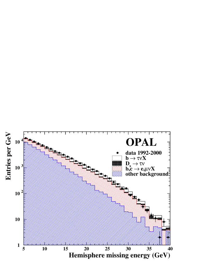
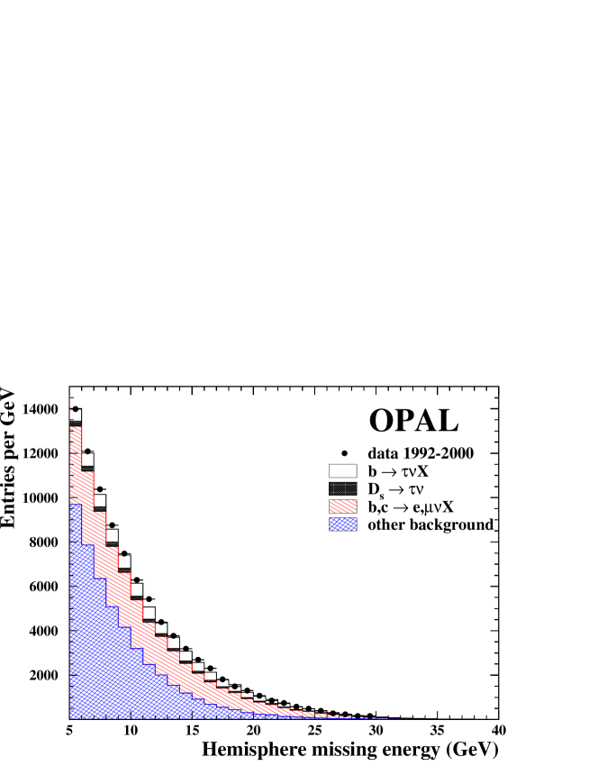
Figure 1: Distribution of the missing energy in a hemisphere, $E_{\rm miss}^{\rm hemi}$, for all selected data events and for the Monte Carlo simulation shown on a logarithmic scale and on a linear scale. The backgrounds from semileptonic heavy quark decays into electrons and muons, and from D${}_{\rm s}^{-}\rightarrow\tau^{-}\overline{\nu}_{\tau}$ decays are shown separately. The number of ${\rm b}\to\tau^{-}\overline{\nu}_{\tau}{\rm X}$ signal events is set to the result of the fit.

A sample of $90587$ hemispheres remains in the data after applying all cuts. Using the Monte Carlo it is estimated to contain about $9\%$ signal events, $3\%$ D${}_{\rm s}^{-}\rightarrow\tau^{-}\overline{\nu}_{\tau}$ decays, $35\%$ non-$\tau$ semileptonic b and c decays, $4\%$ light quark decays and $49\%$ hadronic b and c decays. A large fraction of the semileptonic b and c decays are decays with leptons with momenta below $2$ GeV. Using the $E_{\rm miss}^{\rm hemi}$ distributions predicted by the Monte Carlo simulation for signal and the sum of all backgrounds, a binned maximum likelihood fit is used to determine BR(${\rm b}\to\tau^{-}\overline{\nu}_{\tau}{\rm X}$ ) with the fraction of signal events as the only free parameter. The result of the fit is

$$\mathrm{BR}({{\rm b}\to\tau^{-}\overline{\nu}_{\tau}{\rm X}})=(2.78\pm 0.18)\%,$$ (4)

where the uncertainty takes into account the limited number of Monte Carlo and data events [25]. The result is obtained by fitting the data samples of the different years with the corresponding Monte Carlo samples. The minimum of the fits correspond to $\chi^{2}$ values for $34$ degrees of freedom in the range $31$ to $45$. The $E_{\rm miss}^{\rm hemi}$ distribution for the total data sample is shown in Fig. 1.

5 Systematic uncertainties

The measurement of BR(${\rm b}\to\tau^{-}\overline{\nu}_{\tau}{\rm X}$ ) relies on the Monte Carlo modelling of the missing energy distribution for the signal and background events. Other systematic uncertainties arise from the reproduction of the selection and veto efficiencies for the data in the Monte Carlo simulation and from limited knowledge of the branching ratios for decays involving a heavy quark and a lepton. The sources of systematic uncertainties are described below and their contributions to the total systematic uncertainty are summarised in Table 1.

Source	$\Delta$BR(${\rm b}\to\tau^{-}\overline{\nu}_{\tau}{\rm X}$ )
leptonic $E_{\rm miss}^{\rm hemi}$ description	$-0.16\%$
hadronic $E_{\rm miss}^{\rm hemi}$ description	$+0.15\%$
tracking resolution	$\pm 0.04\%$
calorimeter resolution	$\pm 0.06\%$
b tagging efficiency	$\pm 0.04\%$
e± veto	$\pm 0.11\%$
$\mu^{\pm}$ veto	$\pm 0.07\%$
$\langle x_{\rm b}\rangle=0.702\pm 0.008~{}\cite[cite]{[\@@bibref{}{bib:pr319}{}{}]}$	$\pm 0.33\%$
$\langle x_{\rm c}\rangle=0.484\pm 0.008~{}\cite[cite]{[\@@bibref{}{bib:pr319}{}{}]}$	$\pm 0.04\%$
${\rm b}\to\tau^{-}\overline{\nu}_{\tau}{\rm X}$ decay modelling	$\pm 0.03\%$
semileptonic b decay models	$\pm 0.26\%$
BR(b $\rightarrow\ell^{-}\overline{\nu}{\rm X}$)=($10.73\pm 0.18)\%$ [9]	$\pm 0.08\%$
BR(b $\rightarrow$ c or $\overline{c}\rightarrow\ell\nu{\rm X}$ )=($9.69\pm 0.51)\%$ [26]	$\pm 0.05\%$
BR(D${}_{\rm s}^{-}\rightarrow\tau^{-}\overline{\nu}_{\tau}$)=($7.2\pm 2.3)\%$ [27, 28]	$\pm 0.13\%$
$f({\rm b}\to{\rm D}_{\rm s}^{-})=(18\pm 5)\%)$ [29]	$\pm 0.10\%$
Total systematic uncertainty	$\pm 0.51$%

Table 1: The contributions to the systematic uncertainty on BR(${\rm b}\to\tau^{-}\overline{\nu}_{\tau}{\rm X}$ ).

An imperfect modelling of the signal region of the $E_{\rm miss}^{\rm hemi}$ distribution by the Monte Carlo simulation can bias the result. We have therefore studied the modelling of the $E_{\rm miss}^{\rm hemi}$ distribution using three different signal-depleted control samples: a sample enriched in semileptonic b decays, a sample enriched in hadronic b decays and a light quarks control sample. In these samples, the ratio of the $E_{\rm miss}^{\rm hemi}$ distributions of data and Monte Carlo has been studied. The missing energy distributions for the control samples together with the corresponding Monte Carlo predictions are shown in Fig. 2.

Leptonic control sample:

A sample enriched in semileptonic b decays is selected by using the same requirements for the b-tagging as for the signal sample (Section 3). For the leptonic control sample, hemispheres with electrons and muons are selected and not rejected. To obtain a pure sample, at least one electron or one muon candidate with a high value for the output of the lepton identification neural networks is required. According to the Monte Carlo about $85\%$ of the control sample are semileptonic b and c decays.

The $E_{\rm miss}^{\rm hemi}$ distribution for this class of events is well described by the Monte Carlo simulation (Fig. 2a). To estimate the systematic uncertainty associated with residual differences, the ratio of the data and the Monte Carlo distribution (Fig. 2b) is fitted with a straight line separately for every year of data taking. The largest slope $a$ obtained from these fits is used to reweight the $E_{\rm miss}^{\rm hemi}$ distribution for semileptonic b decays in the Monte Carlo background. The events are reweighted using a weight

$$w(E_{\rm miss}^{\rm hemi})=1+a(E_{\rm miss}^{\rm hemi}-\overline{E}^{\rm hemi}_{\rm miss}),$$ (5)

where $\overline{E}^{\rm hemi}_{\rm miss}$ is the mean of the missing energy distribution. Using a second order polynomial fit instead yields a similar systematic uncertainty.

Hadronic control sample:

To study the description of the missing energy distribution for hadronic b decays, a sample is selected by applying b-tagging, the lepton veto and by requiring at least 10 GeV energy deposit in the hadron calorimeter. These requirements enrich the sample in events with large hadronic energy. The agreement between data and Monte Carlo for the $E_{\rm miss}^{\rm hemi}$ distribution is reasonable in the signal region (Fig. 2c,d). The systematic uncertainty is estimated using the method described above and given in Table 1. It increases if the cut on $E_{\rm miss}^{\rm hemi}$ is reduced (Table 2). To keep the quadratic sum of the statistical and systematic uncertainty small, the cut $E_{\rm miss}^{\rm hemi}>5$ GeV is chosen. All other relevant systematic uncertainties show only a small dependence on the $E_{\rm miss}^{\rm hemi}$ cut.

$E_{\rm miss}^{\rm hemi}$ cut	stat	syst
(GeV)
0	$\pm 0.14\%$	$+1.00\%$
3	$\pm 0.16\%$	$+0.45\%$
5	$\pm 0.18\%$	$+0.15\%$
7	$\pm 0.21\%$	$+0.09\%$
9	$\pm 0.27\%$	$+0.08\%$

Table 2: The statistical and the systematic uncertainty on the measurement of BR(${\rm b}\to\tau^{-}\overline{\nu}_{\tau}{\rm X}$ ) due to the Monte Carlo description for events with hadronic b and c decays for different fitting ranges.

Light quarks control sample:

A further test of the Monte Carlo description of the $E_{\rm miss}^{\rm hemi}$ distribution is performed for a light quark (uds) flavour sample. The sample is selected by exploiting the fact that events with a hadron carrying reconstructed momentum between 0.5 and 1.07 of the beam momentum mostly originate from uds primary quarks [30]. The light quark tag is applied in the opposite hemisphere. The $E_{\rm miss}^{\rm hemi}$ distribution for this sample is shown in Fig. 2e. Reweighting the light quark background events according to Eq. 5 results in a negligible contribution to the total systematic uncertainty.

Detector effects:

The description of the visible energy distribution depends on a correct reproduction of the detector resolution in the Monte Carlo samples. The tracking resolution has been modified by $\pm 10\%$ to evaluate the systematic uncertainty [22]. The energy scale of the electromagnetic calorimeter (ECAL) is varied according to the small shift between the mean of the ECAL energy distributions in data and Monte Carlo found for an inclusive sample of hadronic Z decays. The uncertainty obtained by varying the resolution by $\pm 10\%$ is found to be even smaller. The estimated uncertainties are listed in Table 1.

Figure 2: Comparison of the distributions of the missing energy in a hemisphere, $E_{\rm miss}^{\rm hemi}$, between the data taken in 1994 and the Monte Carlo simulation for the three control samples: a,b) leptonic control sample; c,d) hadronic control sample; e,f) light quarks control sample (see text). The number of hemispheres in the Monte Carlo is normalised to the number of hemispheres in the data. The lines indicate the weight function $w(E_{\rm miss}^{\rm hemi})$ (Eq. 5) for the fitted slopes $a$ and for $a=0$, i.e. perfect agreement between data and Monte Carlo simulation for the control samples.

The following systematic uncertainties are related to the modelling of the cuts:

b-tagging efficiency:

The b-tagging efficiency is checked by comparing the fraction of events with one and two tagged hemispheres in data and Monte Carlo. Using the hemisphere correlation from the Monte Carlo simulation a b-tagging efficiency of $45.7\%$ is obtained using the data compared to $47\%$ using the Monte Carlo, i.e. the Monte Carlo is overestimating the b-tagging efficiency by approximately $3\%$. This result is consistent with similar recent studies [20]. The b-tagged events are reweighted according to this change in efficiency and the systematic shift is found to be negligible, so no correction is applied. In addition, the uncertainty on the rejection efficiencies for the other flavours is evaluated by changing the efficiencies by $10\%$. Since the b-tagging is applied in the opposite hemisphere and the contamination of non-b flavours in the selected sample is below $10\%$, the contribution to the total systematic uncertainty is small.

Lepton identification:

An important background with missing energy due to neutrinos originates from semileptonic decays of b and c quarks to muons or electrons. In [24, 22], the systematic uncertainties on the efficiencies for identifying muons or electrons determined by the Monte Carlo are found to be $5\%$ and $4\%$. This uncertainty is taken into account in the efficiency for rejecting hemispheres with electrons or muons.

The systematic uncertainties due to the other selection cuts are negligible. The remaining errors are due to fragmentation parameters and decay rates which have to be taken from other measurements.

Heavy quark fragmentation and decay modelling:

The distribution of the missing energy depends on the b fragmentation modelling. The effect of the uncertainty is determined by reweighting the Monte Carlo events to reproduce the experimental uncertainty on the mean energy of the b hadrons, $\langle x_{\rm b}\rangle$ using Peterson fragmentation and two other fragmentation models [32, 33]. This variation produces a different energy distribution for the b hadron decay products, resulting in the largest systematic uncertainty.

Since only about $5\%$ of the sample is expected to be Z$\to{\rm c}\bar{\rm c}$ events, the uncertainty on $\langle x_{\rm c}\rangle$ yields only a small contribution to the total systematic uncertainty.

HQET calculations to order $1/m_{\mathrm{b}}^{2}$ show that the $\tau$ polarisation changes by $4\%$ compared to the free quark decay model used in the simulation. A change in polarisation leads to a different $\tau$ energy spectrum. To estimate the effect of non-zero HQET parameters $\lambda_{1}$ and $\lambda_{2}$, the polarisation of the $\tau$ leptons in the Monte Carlo simulation is varied by $4\%$ resulting in a systematic uncertainty of $0.03\%$.

Semileptonic decay models:

A large part of the background is composed of semileptonic b decays where the leptons have a momentum smaller than $2$ GeV. Both the fraction of these decays and the shape of the missing energy distribution depend on their modelling. The ACCMM model [34] is used for the measurement. Using the ISGW [35] model changes the result by $+0.14\%$ and using the ISGW** [36] model changes the result by $-0.26\%$. The larger of the two variations is used as an estimate of the systematic uncertainty.

Uncertainties on decay rates:

The branching fractions of the Z boson into ${\rm c}\bar{\rm c}$ and ${\rm b}\bar{\rm b}$ pairs in hadronic events, $R_{\rm c}$ and $R_{\rm b}$, are taken from [26]. The variation of $R_{\rm c}$ and $R_{\rm b}$ within their uncertainties yields a negligible contribution to the systematic uncertainty. The only significant background involving $\tau$ leptons originates from D${}_{\rm s}^{-}\rightarrow\tau^{-}\overline{\nu}_{\tau}$ decays. Averaging a recent measurement [27] with the measurement in [28], we obtain ${\rm BR}(\mbox{D${}_{\rm s}^{-}\rightarrow\tau^{-}\overline{\nu}_{\tau}$})=(7.2\pm 2.3)\%$. The branching fraction of b quarks into ${\rm D}_{\rm s}^{-}$ is $f({\rm b}\to{\rm D}_{\rm s}^{-})=(18\pm 5)\%)$ [29]. These uncertainties and the uncertainties on the semileptonic branching fractions BR(b $\rightarrow\ell^{-}\overline{\nu}{\rm X}$) and BR(b $\rightarrow$ c or $\overline{c}\rightarrow\ell\nu{\rm X}$ ) have been taken into account by reweighting the Monte Carlo events using the branching fractions and the uncertainties given in Table 1.

6 Results

Using about $3.70$ million hadronic ${\rm Z}$ decays we have measured the inclusive branching ratio:

$$\mathrm{BR}({{\rm b}\to\tau^{-}\overline{\nu}_{\tau}{\rm X}})=(2.78\pm 0.18\pm 0.51)\%.$$ (6)

The size of the total uncertainty is similar to the uncertainties of the measurements in [1-3].

A contribution from charged Higgs decays is expected to enhance the branching ratio compared to that in the Standard Model. Since we have found no large enhancement of the branching ratio compared to the Standard Model prediction $\mathrm{BR}({{\rm b}\to\tau^{-}\overline{\nu}_{\tau}{\rm X}})=(2.36\pm 0.17)\%$, we set a constraint on such a contribution for Type II Two Higgs Doublet Models [7].

The $\tau$ polarisation depends on the Higgs contribution and can be calculated as a function of $r=\tan\beta/M_{{\rm H}^{\pm}}$ [7]. This is taken into account by an iterative procedure for the limit calculation. A limit of $r<0.52$ GeV^-1 is obtained assuming $\tau$ polarisation as for the Standard Model decay. The polarisation of the $\tau$ leptons in the Monte Carlo simulation is changed according to this value of $r$ and the limit is recalculated. The resulting limit is

$$\frac{\tan\beta}{M_{{\rm H}^{\pm}}}<0.53\ {\rm GeV}^{-1}$$ (7)

at $95\%$ confidence level.

References

-
[1]
ALEPH Collab., R. Barate et al., Eur. Phys. J. C19 (2001) 213.
. -
[2]
DELPHI Collab., P. Abreu et al., Phys. Lett. B496 (2000) 43.
(). -
[3]
L3 Collab., M. Acciarri et al., Phys. Lett. B332 (1994) 201.
(). - [4] A. Falk, Z. Ligeti, M. Neubert and Y. Nir, Phys. Lett. B326 (1994) 145.
- [5] Z. Ligeti and Y. Nir, Phys. Rev. D49 (1994) 4331.
-
[6]
P. Krawczyk and S. Pokorski, Phys. Rev. Lett. 60 (1988) 182;
B. Grzadkowski and W.S. Hou, Phys. Lett. B272 (1991) 383;
G. Isidori, Phys. Lett. B 298 (1992) 409. -
[7]
Y. Grossman and Z. Ligeti, Phys. Lett. B 332 (1994) 373;
Y. Grossman, H.E. Haber and Y. Nir, Phys. Lett. B357 (1995) 630. - [8] J. A. Coarasa, R. A. Jimenez and J. Sola, Phys. Lett. B406 (1997) 337.
- [9] The Particle Data Group, D.E. Groom et al., Eur. Phys. J. C15 (2000).
-
[10]
OPAL Collab., K. Ahmet et al., Nucl. Instr. and Meth. A305 (1991) 275;
P.P. Allport et al., Nucl. Instr. and Meth. A346 (1994) 476;
P.P. Allport et al., Nucl. Instr. and Meth. A324 (1993) 34;
O. Biebel et al., Nucl. Instr. and Meth. A323 (1992) 169;
M. Hauschild et al., Nucl. Instr. and Meth. A314 (1992) 74;
B.E. Anderson et al., IEEE Trans. Nucl. Sci. 41 (1994) 845. - [11] OPAL Collab., G. Alexander et al., Z. Phys. C52 (1991) 175.
- [12] OPAL Collab., R. Akers et al., Z. Phys. C65 (1995) 17.
- [13] T. Sjöstrand, Comp. Phys. Comm. 82 (1994) 74.
- [14] C. Peterson, D. Schlatter, I. Schmitt and P. Zerwas, Phys. Rev. D27 (1983) 105.
- [15] OPAL Collab., G. Alexander et al., Z. Phys. C69 (1996) 543.
-
[16]
M. Jeżabek and L. Motyka, Nucl. Phys. B501 (1997) 207;
M. Jeżabek and P. Urban, Nucl. Phys. B525 (1998) 350. - [17] S. Jadach, Z. Wa̧s, R. Decker and J.H. Kühn, Comp. Phys. Comm. 76 (1993) 361.
- [18] J. Allison et al., Nucl. Instr. Meth. A317 (1992) 47.
-
[19]
S. Brandt et al., Phys. Lett. 12 (1964) 57;
E. Fahri, Phys. Rev. Lett. 39 (1977) 1587. -
[20]
OPAL Collab., G. Abbiendi et al., Eur. Phys. J. C7 (1999) 407;
OPAL Collab., G. Abbiendi et al., Eur. Phys. J. C12 (2000) 567. - [21] OPAL Collab., G. Alexander et al., Phys. Lett. B377 (1996) 181.
- [22] OPAL Collab., G. Abbiendi et al., Eur. Phys. J. C8 (1999) 217.
- [23] OPAL Collab., R. Akers et al., Z. Phys. J. C66 (1995) 19.
- [24] OPAL Collab., G. Abbiendi et al., Eur. Phys. J. C16 (2000) 41.
- [25] R. Barlow and C. Beeston, Comp. Phys. Comm. 77 (1993) 219.
- [26] ALEPH, DELPHI, L3, OPAL, CDF and SLD Collab., “Combined results on b-hadron production rates, lifetimes, oscillations and semileptonic decays”, CERN-EP-2000-096.
- [27] OPAL Collab., G. Abbiendi et al., “Measurement of the Branching Ratio for D Decays”, CERN-EP-2001-019, accepted by Phys. Lett. B.
- [28] L3 Collab., M. Acciarri et al., Phys. Lett. B396 (1997) 327.
- [29] ALEPH Collab., D. Busculic et al., Phys. Lett. B388 (1996) 648.
- [30] OPAL Collab., R. Akers et al., Z. Phys. C60 (1993) 397.
- [31] OPAL Collab., G. Abbiendi et al., Eur. Phys. J. C13 (2000) 225.
- [32] P. Collins and T. Spiller. J. Phys. G11 (1985) 1289.
- [33] V.G. Kartvelishvili, A.K. Likehoded and V.A. Petrov, Phys. Lett. B78 (1978) 615.
- [34] G. Altarelli, N. Cabibbo, G. Corbò, L. Maiani and G. Martinelli, Nucl. Phys. B208 (1982) 365.
- [35] N. Isgur, D. Scora, B. Grinstein and M. Wise, Phys. Rev. D39 (1989) 799.
- [36] CLEO Collab., R. Fulton et al., Phys. Rev. D43 (1991) 651.