REVIEW OF B PHYSICS RESULTS
FROM THE LEP EXPERIMENTS AND SLD

Abstract

A review of b physics results from the LEP experiments and SLD is presented. Emphasis is given to the determinations of the $|{\mathrm{V}}_{\mathrm{cb}}|$ and $|{\mathrm{V}}_{\mathrm{ub}}|$, and to the study of B meson oscillations, which yield bounds on the unitarity triangle.

1 Introduction

Over the past decade, many important b physics measurements were performed at Z factories (LEP, SLC). The large boost of b hadrons gives access to important properties (e.g. lifetimes, oscillation frequencies of neutral B mesons), which cannot be studied with b hadrons at rest. Today asymmetric B factories are taking over for what concerns the physics of ${\mathrm{B}}^{0}$ and ${\mathrm{B}}^{+}$ mesons, while our experimental knowledge of ${\mathrm{B}}^{0}_{\mathrm{s}}$ and b baryon physics is still based on measurements performed by the LEP experiments and SLD, and by CDF at the Tevatron. A major step forward in these topics will be made only when significant statistics from the Tevatron Run II are analyzed. In this review emphasis is given to studies of b decay properties rather than b hadron production; in particular to measurements that are related to the determination of CKM matrix elements, and hence to the description of CP violation in the Standard Model.

First, results on b hadron lifetimes are reviewed. The inclusive b lifetime is an input parameter for the derivation of $|{\mathrm{V}}_{\mathrm{cb}}|$ and $|{\mathrm{V}}_{\mathrm{ub}}|$ from the inclusive semileptonic branching ratios, while individual b-hadron lifetimes provide an important test of our understanding of hadron dynamics. The lifetime difference in the ${\mathrm{B}}^{0}_{\mathrm{s}}$ system is now also measured; the ratio to the oscillation frequency can be calculated on the lattice. Next, measurements of inclusive semileptonic b decay rates are presented, which give the opportunity to derive $|{\mathrm{V}}_{\mathrm{cb}}|$ and $|{\mathrm{V}}_{\mathrm{ub}}|$. An alternative determination of $|{\mathrm{V}}_{\mathrm{cb}}|$ is provided by the study of ${\mathrm{B}}\to{\mathrm{D}}^{\star}\ell\nu$ exclusive decays. Finally, studies of neutral B meson oscillations yield information on $|{\mathrm{V}}_{\mathrm{td}}|$ and $|{\mathrm{V}}_{\mathrm{ts}}|$.

Most of the results presented are based on analyses from the LEP experiments and SLD. The LEP I data sample consists of almost four million hadronic decays per experiment. SLD has collected a sample 10 times smaller than that of each LEP experiment, but is competitive on some specific analyses, due to some unique features of the accelerator and the detector. The polarization of the electron beam, the tiny and stable beam spot and the excellent precision of the CCD vertex detector significantly enhance the quark charge tagging capability, the precision in the track impact paremeter and b decay length measurements, and the efficiency in inclusive secondary vertex finding.

2 Measurements of b hadron lifetimes

Measurements of the inclusive b lifetime are based on semileptonic or fully inclusive final states, either measuring the impact parameter of charged particle tracks, or the decay length of inclusively reconstructed secondary vertices.

Individual b hadron lifetimes are measured with several techniques. The most precise results come from reconstruction of semileptonic final states and from inclusive reconstruction of secondary vertices, particularly suitable for ${\mathrm{B}}^{+}$ mesons. The averages of results from CDF, SLD and the LEP experiments are shown in Fig. 1a; the ratio of individual lifetimes to the ${\mathrm{B}}^{0}$ lifetimes are compared with theoretical predictions[1] in Fig. 1b. The predicted hyerarchy is observed. The difference between the ${\mathrm{B}}^{0}$ and ${\mathrm{B}}^{+}$ lifetimes is established experimentally at more than $3\sigma$. A discrepancy between measurement and prediction of about $3\sigma$ emerges for the b baryon lifetime.

Figure 1: (a) Experimental results for inclusive and individual b hadron lifetimes. The averages include all analyses from CDF, SLD and the LEP experiments. (b) Comparison of lifetime ratios with theoretical predictions.

New measurements of ${\mathrm{B}}^{0}$ and ${\mathrm{B}}^{+}$ lifetimes are now coming from the asymmetric B factories: the precision of the results presented here is expected to be exceeded by the end of 2001. For ${\mathrm{B}}^{0}_{\mathrm{s}}$ and b baryon lifetimes, no significant improvement is to be expected from new analyses of the available data samples.

The discrepancy between theory and experiments for the b baryon lifetime has triggered new theoretical studies. Neubert[2] has performed an analysis with less modelling assumptions, varying the unknown hadronic matrix elements within plausible ranges. The predictivity for the hyerarchy between ${\mathrm{B}}^{0}$ and ${\mathrm{B}}^{+}$ is lost, and the low measured value of the baryon lifetime is still difficult to accommodate. Analyses based on QCD sum rules[3] also give a prediction higher than the measurement, although Huang et al.[4], by stretching some assumptions, have been able to produce a low value, $\tau(\Lambda_{\mathrm{b}})/\tau({\mathrm{B}}^{0})=0.86\pm 0.04$, in better agreement with the experimental determination.

Several methods have been explored by the LEP experiments and CDF to constrain the lifetime difference in the ${\mathrm{B}}^{0}_{\mathrm{s}}$ system. The simplest analyses are based on the observation that fitting for the ${\mathrm{B}}^{0}_{\mathrm{s}}$ lifetime in inclusive samples, or samples of semileptonic ${\mathrm{B}}^{0}_{\mathrm{s}}$ decays, yields a result which takes a second order correction from a possible lifetime difference bewteen the two ${\mathrm{B}}^{0}_{\mathrm{s}}$ states. Assuming that the ${\mathrm{B}}^{0}_{\mathrm{s}}$ and ${\mathrm{B}}^{0}$ decay widths are equal ($\Gamma_{\mathrm{s}}=\Gamma_{\mathrm{d}}$), the result can be translated to a constraint on the lifetime difference. Alternatively, the selection can be aimed at enhancing the ${\mathrm{B}}^{0}_{\mathrm{s}}$ short content of the sample analysed. In this case the fraction of ${\mathrm{B}}^{0}_{\mathrm{s}}$ short has to be evaluated, and the sensitivity of the fitted lifetime to the lifetime difference is higher. Finally, ALEPH tried to select ${\mathrm{D}}_{\mathrm{s}}^{+}{\mathrm{D}}_{\mathrm{s}}^{-}$ final states, corresponding to ${\mathrm{B}}^{0}_{\mathrm{s}}$ short decays, by selecting jets containing two reconstructed $\phi$ mesons. Fitting for the lifetime of this sample yields a direct measurement of the ${\mathrm{B}}^{0}_{\mathrm{s}}$ short lifetime. In addition, since this final state is the only significant contribution to the width difference, a measurement of the rate can also be translated to a constraint on the lifetime difference. All these methods yield rather mild constraints on the ${\mathrm{B}}^{0}_{\mathrm{s}}$ lifetime difference, but combining the likelihood profiles from all the analyses, together with the contraint $\Gamma_{\mathrm{s}}=\Gamma_{\mathrm{d}}$, gives the result reported in Fig. 2, which can be quantified either as a measurement or as a 95% C.L. limit:

$$\Delta\Gamma_{\mathrm{s}}/\Gamma_{\mathrm{s}}=0.16\,^{+0.08}_{-0.09}\ ,\ \ \ \ \ \ \ \ \ \Delta\Gamma_{\mathrm{s}}/\Gamma_{\mathrm{s}}<0.31\,@\ 95\%\ {\mathrm{C.L.}}\ ,$$ (1)

in good agreement with the theoretical prediction[5] of $\Delta\Gamma_{\mathrm{s}}/\Gamma_{\mathrm{s}}=0.097\,^{+0.038}_{-0.050}$.

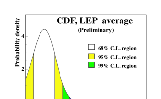
Figure 2: Probability density function for $\Delta\Gamma_{\mathrm{s}}/\Gamma_{\mathrm{s}}$ from all available analyses, with the additional constraint $\Gamma_{\mathrm{s}}=\Gamma_{\mathrm{d}}$.

3 Semileptonic decays

The inclusive direct semileptonic decay rate of b hadrons ${\mathrm{BR}}({\mathrm{b}}\to{\mathrm{X}}\ell\nu)$ is measured by the LEP experiments. High-purity b hadron samples are obtained by applying a lifetime tagging in the opposite event-half, while a reliable knowledge of the lepton identification and background is achieved thanks to several control samples which allow the simulation to be precisely tuned with the data. The challenge of these analyses is to disentangle the various sources of prompt leptons in b decays, in particular direct ${\mathrm{b}}\to{\mathrm{X}}\ell\nu$ from cascade ${\mathrm{b}}\to{\mathrm{c}}\to{\mathrm{X}}\ell\nu$ decays, keeping control of the related systematic uncertainties.

The measurements available are reported in Fig. 3, together with the average. Two new results from ALEPH have been recently released, obtained with methods that have largely independent systematic uncertainties.

Figure 3: Measurements of ${\mathrm{BR}}({\mathrm{b}}\to{\mathrm{X}}\ell\nu)$ at LEP, and combined value.

The ${\mathrm{BR}}({\mathrm{b}}\to{\mathrm{X}}\ell\nu)$ value, together with the measurement of the inclusive b lifetime, yield a determination of the $|{\mathrm{V}}_{\mathrm{cb}}|$[1], once the small ${\mathrm{b}}\to{\mathrm{X}}_{\mathrm{u}}\ell\nu$ contribution has been subtracted,

$$|{\mathrm{V}}_{\mathrm{cb}}|=(41.1\pm 2.5)\times 10^{-3}\times\sqrt{\frac{{\mathrm{BR}}({\mathrm{b}}\to{\mathrm{X}}_{\mathrm{c}}\ell\nu)}{0.105}}\times\sqrt{\frac{1.55\ {\mathrm{ps}}}{\tau_{\mathrm{b}}^{\mathrm{incl}}}}\ ,$$ (2)

obtaining

$$|{\mathrm{V}}_{\mathrm{cb}}|=(40.9\ \pm\,0.5_{\mathrm{exp}}\ \pm\,2.4_{\mathrm{theo}})\times 10^{-3}\ ,$$ (3)

where the uncertainty is dominated by the theoretical error from Eq. 2. The ${\mathrm{BR}}({\mathrm{b}}\to{\mathrm{X}}\ell\nu)$ result from LEP can also be compared with the $\Upsilon{\mathrm{(4S)}}$ value, after correcting for the different b hadron mixture. Assuming equal semileptonic widths for all b species, the correction can be written as

$${\left.{\mathrm{BR}}({\mathrm{B}}\to{\mathrm{X}}\ell\nu)\right|}_{\mathrm{LEP}}={\mathrm{BR}}({\mathrm{b}}\to{\mathrm{X}}\ell\nu)\times\frac{\tau_{\mathrm{B}}}{\tau_{\mathrm{b}}}=0.1085\pm 0.0027\ ,$$ (4)

which compares rather well with the value measured by CLEO[6]

$${\left.{\mathrm{BR}}({\mathrm{B}}\to{\mathrm{X}}\ell\nu)\right|}_{\mathrm{CLEO}}=0.1049\pm 0.0046\ .$$ (5)

An alternative determination of $|{\mathrm{V}}_{\mathrm{cb}}|$ is provided by the study of exclusive ${\mathrm{B}}\to{\mathrm{D}}^{\star}\ell\nu$ decays. The decay rate can be written as a function of the ${\mathrm{D}}^{\star}$ boost in the ${\mathrm{B}}$ rest frame $\omega$, as[7]

$$\frac{d\Gamma}{d\omega}\propto{\cal{K}}(\omega){\cal{F}}^{2}(\omega)|{\mathrm{V}}_{\mathrm{cb}}|^{2}\ ,$$ (6)

where ${\cal{K}}(\omega)$ is a phase space factor and ${\cal{F}}(\omega)$ is an unknown hadronic form factor. In the infinite b quark mass limit, the hadronic form factor equals unity for a ${\mathrm{D}}^{\star}$ at rest ($\omega=1$). Mass and non-perturbative corrections can be calculated with the Operator Product Expansion formalism[1], obtaining ${\cal{F}}(1)=0.88\pm 0.05$. In the analyses the spectrum of the candidates as a function of the reconstucted $\omega$ is fit for the slope $\rho^{2}$ and the intecept at $\omega=1$, ${\cal{F}}(1)|{\mathrm{V}}_{\mathrm{cb}}|$, where the phase space vanishes. The results are averaged accounting for the correlation between the two free parameters, obtaining the results shown in Fig. 4a. The determintation from the exclusive channel is in perfect agreement with that from the inclusive ${\mathrm{b}}\to{\mathrm{X}}\ell\nu$ rate, as shown in Fig.4b, where a global average is also presented.

Figure 4: (a) Measurements of ${\cal{F}}(1)|{\mathrm{V}}_{\mathrm{cb}}|$,${\mathrm{BR}}({\mathrm{b}}\to{\mathrm{X}}\ell\nu)$ at LEP, and combined value. (b) Inclusive and exclusive determination of $|{\mathrm{V}}_{\mathrm{cb}}|$, along with their combination; the first error quoted comes from the uncertainties on the experimental inputs, the second from theory.

The LEP experiments have also performed analyses of inclusive semileptonic decays, where charmed and charmless hadronic final states are discriminated on a statistical basis, producing measurements ${\mathrm{BR}}({\mathrm{b}}\to{\mathrm{X}}_{\mathrm{u}}\ell\nu)$. Discriminating variables are aimed at selecting low-mass hadronic states; the task is complicated by the high multiplicity of fragmentation particles, which need to be disentangled from the b decay products. The analyses try to achieve the best possible separation between charmed and charmless final states by combining several discriminating variables by means of neural networks. Nevertheless the signal is measured on top of a large background from ${\mathrm{b}}\to{\mathrm{X}}_{\mathrm{c}}\ell\nu$ transitions, which need to be subtracted; the estimate of the related systematic uncertainties is the critical issue for these analyses. On the other hand, because the b hadron has a large boost, the selection has relatively small dependence upon the decay kinematics, and therefore upon the modelling of the signal. The results available and the LEP average are shown in Fig. 5.

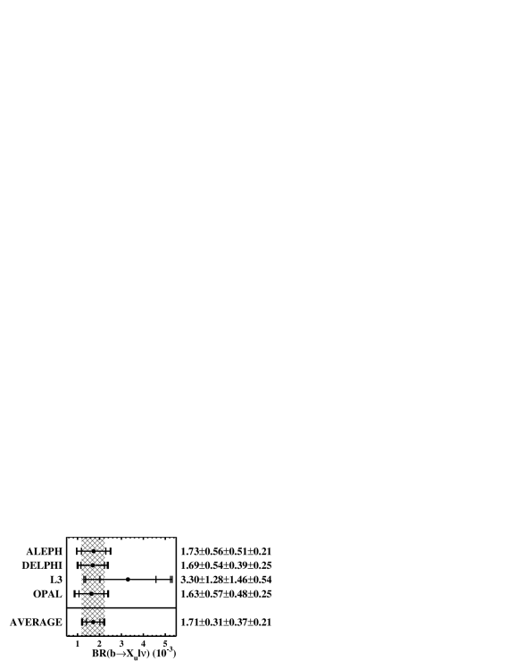
Figure 5: Measurements of ${\mathrm{BR}}({\mathrm{b}}\to{\mathrm{X}}_{\mathrm{u}}\ell\nu)$ at LEP, and combined value. The first uncertainty quoted accounts for limited statistics and detector effects, the second for the modelling of the ${\mathrm{b}}\to{\mathrm{X}}_{\mathrm{c}}\ell\nu$ background and the third for the modelling of the ${\mathrm{b}}\to{\mathrm{X}}_{\mathrm{u}}\ell\nu$ signal.

Similarly to Eq. 2, the measured branching ratio can be used to extract the $|{\mathrm{V}}_{\mathrm{ub}}|$[8] according to

$$|{\mathrm{V}}_{\mathrm{ub}}|=(4.45\pm 0.18)\times 10^{-3}\times\sqrt{\frac{{\mathrm{BR}}({\mathrm{b}}\to{\mathrm{X}}_{\mathrm{u}}\ell\nu)}{0.002}}\times\sqrt{\frac{1.55\ {\mathrm{ps}}}{\tau_{\mathrm{b}}^{\mathrm{incl}}}}\ ,$$ (7)

which yields

$$|{\mathrm{V}}_{\mathrm{ub}}|=(4.09\ {{}^{+0.36}_{-0.39}}_{\mathrm{stat+exp}}\ {{}^{+0.42}_{-0.47}}_{\mathrm{b\to c}}\ {{}^{+0.24}_{-0.26}}_{\mathrm{b\to u}}\ \pm\,0.17_{\mathrm{theo}})\times 10^{-3}\ ,$$ (8)

where the first error accounts for limited statistics and detector effects, the second and third come from the modelling of ${\mathrm{b}}\to{\mathrm{X}}_{\mathrm{c}}\ell\nu$ and ${\mathrm{b}}\to{\mathrm{X}}_{\mathrm{u}}\ell\nu$ transitions, respectively, and the last reflects the uncertainty in Eq. 7.

4 Neutral B meson oscillations

The oscillation frequency in the ${\mathrm{B}}^{0}-\overline{{\mathrm{B}}^{0}}$ system, which is proportional to the mass difference of the two eigenstates, can be translated to a measurement of $|{\mathrm{V}}_{\mathrm{td}}|$, $\Delta m_{\mathrm{d}}\propto{|{\mathrm{V}}_{\mathrm{td}}|}^{2}\times({\mathrm{QCD\ corrections}})$, yielding a constraint on the size of the CP violating phase $\eta$. Unfortunately QCD effects are large and the associated uncertainty dominates the extraction of ${\mathrm{V}}_{\mathrm{td}}$. A better constraint on $\eta$ could be obtained from the ratio of the oscillation frequencies of ${\mathrm{B}}^{0}_{\mathrm{s}}$ and ${\mathrm{B}}^{0}$ mesons, since some of the QCD uncertainties cancel in the ratio. The factor $\xi$ in Eq. 9 is estimated to be known at the $5\%$ level.

$$\frac{\Delta m_{\mathrm{s}}}{\Delta m_{\mathrm{d}}}=\frac{m_{{\mathrm{B}}^{0}_{\mathrm{s}}}}{m_{{\mathrm{B}}^{0}}}\xi^{2}{\left|\frac{{\mathrm{V}}_{\mathrm{ts}}}{{\mathrm{V}}_{\mathrm{td}}}\right|}^{2}\ .$$ (9)

The proper time distributions of “mixed” and “unmixed” decays, given in Eq. 10, are measured experimentally. The oscillating term introduces a time-dependent difference between the two classes.

$${\cal P}(t)_{{\mathrm{B}}^{0}_{\mathrm{q}}\to\overline{{\mathrm{B}}^{0}_{\mathrm{q}}}} = \frac{\Gamma e^{-\Gamma t}}{2}\,[1-\cos(\Delta m_{\mathrm{q}}\,t)]\ ,$$

$${\cal P}(t)_{{\mathrm{B}}^{0}_{\mathrm{q}}\to{\mathrm{B}}^{0}_{\mathrm{q}}} = \frac{\Gamma e^{-\Gamma t}}{2}\,[1+\cos(\Delta m_{\mathrm{q}}\,t)]\ ,$$ (10)

The amplitude of such difference is damped not only by the natural exponential decay, but also by the effect of the experimental resolution in the proper time determination. The proper time is derived from the measured decay length and the reconstructed momentum of the decaying meson. The resolution on the decay length $\sigma_{L}$ is to first order independent of the decay length itself, and is largely determined by the tracking capabilities of the detector. The momentum resolution $\sigma_{p}$ depends strongly on the final state chosen for a given analysis, and is typically proportional to the momentum itself.

Figure 6: Difference in the proper time distributions of unmixed and mixed decays for monochromatic ${\mathrm{B}}$ mesons, fixed decay length and momentum resolutions, and different values of the oscillation frequency.

The proper time resolution can be therefore written as:

$$\sigma_{t}=\frac{m}{p}\sigma_{L}\oplus\frac{\sigma_{p}}{p}\,t\ ,$$ (11)

where the decay length resolution contributes a constant term, and the momentum resolution a term proportional to the proper time. Examples of the resulting observable difference are shown in Fig. 6, for the simple case of monochromatic ${\mathrm{B}}$ mesons of momentum $32\ {\mathrm{GeV}}\!/\!c$, resolutions of $\sigma_{p}/p=0.15$ and $\sigma_{L}=250\ \mu{\mathrm{m}}$ (Gaussian), and for different values of the true oscillation frequency. For low frequency several periods can be observed. As the frequency increases, the effect of the finite proper time resolution becomes more relevant, inducing an overall decrease of observed difference, and a faster damping as a function of time (due to the momentum resolution component). In the example given, for a frequency of $25\ {\mathrm{ps}}^{-1}$ only a small effect corresponding to the first half-period can be seen.

The first step for a ${\mathrm{B}}$ meson oscillation analysis is the selection of final states suitable for the study. The choice of the selection criterion determines also the strategy for the tagging of the meson flavour at decay time. Then, the flavour at production time is tagged, to give the global mistag probability. Finally, the proper time is reconstructed for each meson candidate, and the oscillation is studied by means of a likelihood fit to the distributions of decays tagged as mixed or unmixed.

Figure 7: Measurements of $\Delta m_{\mathrm{d}}$ from the LEP experiments, SLD and CDF, with the average from high-energy colliders.

Several measurements of the ${\mathrm{B}}^{0}$ oscillations frequency have been produced by the LEP experiments, SLD and CDF. A variety of selection methods have been used, offering different advantages in terms of statistics, signal purity and control of the systematic uncertainties. The average per experiment, and the global average are shown in Fig. 7. All the analyses rely on the simulation to some extent, and therefore are affected by uncertainties in the physics processes that are simulated. The results are adjusted to a common set of input parameters (e.g. b hadron lifetimes and production fractions) and then averaged, deriving the result of Fig. 7 and the following values for the b hadron production fractions:

$$f_{{\mathrm{B}}^{0},{\mathrm{B}}^{+}}=(40.0\pm 1.0)\%\ \ \ \ \ f_{{\mathrm{B}}^{0}_{\mathrm{s}}}=(9.7\pm 1.2)\%\ \ \ \ \ f_{\mathrm{baryon}}=(10.3\pm 1.7)\%\ .$$ (12)

In the case of ${\mathrm{B}}^{0}_{\mathrm{s}}$ oscillations, the analyses currently available have not been able to resolve the oscillation and produce a measurement of the frequency; only certain ranges of frequencies have been excluded. Combining such excluded ranges is not straightforward, and a specific method, the amplitude method, was introduced for this purpose[9]. In the likelihood fit to the proper time distribution of decays tagged as mixed or unmixed, the frequency of the oscillation is not taken to be the free parameter, but it is instead fixed to a “test” value $\omega$. An auxiliary parameter, the amplitude ${\cal{A}}$ of the oscillating term is introduced, and left free in the fit. The proper time distributions for mixed and unmixed decay, prior to convolution with the experimental resolution, are therefore written as

$${\cal P}(t)=\frac{\Gamma e^{-\Gamma t}}{2}\,[1\pm{\cal{A}}\cos(\omega\,t)]\ ,$$ (13)

with $\omega$ the test frequency and ${\cal{A}}$ the only free parameter. When the test frequency is much smaller than the true frequency ($\omega\ll\Delta m_{\mathrm{s}}$) the expected value for the amplitude is ${\cal{A}}=0$. At the true frequency ($\omega=\Delta m_{\mathrm{s}}$) the expectation is ${\cal{A}}=1$. All the values of the test frequency $\omega$ for which ${\cal{A}}+1.645\sigma_{\cal{A}}<1$ are excluded at $95\%$ C.L. When $\omega$ approaches or exceeds the true frequency $\Delta m_{\mathrm{s}}$, the shape of ${\cal{A}}(\omega)$ depends on the details of the analysis and can be calculated analytically in simple cases[10]. The amplitude has well-behaved errors, and different measurements can be combined in a straightforward way, by averaging the amplitude measured at different test frequencies. The excluded range is derived from the combined amplitude scan.

At present the world combination is dominated at high frequency by the analyses of ALEPH and SLD. The amplitude spectrum, with statistical and systematic errors is shown in Fig. 8a. A lower limit of $\Delta m_{\mathrm{s}}>14.6\ {\mathrm{ps}}^{-1}$ is derived, while the expected limit (sensitivity) is $\Delta m_{\mathrm{s}}>18.3\ {\mathrm{ps}}^{-1}$. The difference is due to the positive amplitude values measured around $17\ {\mathrm{ps}}^{-1}$, compatible with one, as expected in the presence of signal. The error on the amplitude at high frequency ($\Delta m_{\mathrm{s}}\approx 20\ {\mathrm{ps}}^{-1}$) is reduced by about a factor of two compared to the world combination of Summer 1999, mostly because of improvements in the analysis techniques. Some improvements are still expected both from the the LEP experiments and SLD.

Figure 8: (a) Combined amplitude spectrum as a function of test frequency $\omega$. (b) Log-likelihood profile as derived from the amplitude spectrum (world combination). The dashed lines would represent the $1-2\ \sigma$ levels, if the likelihood was parabolic in a range wide enough around the minimum.

The amplitude spectrum can be translated to a log-likelihood profile, referred to the asymptotic value for $\Delta m_{\mathrm{s}}\to\infty$ (Fig.8b). A minimum is observed at $\Delta m_{\mathrm{s}}\approx 17\ {\mathrm{ps}}^{-1}$. The deviation of the measured amplitude from ${\cal{A}}=0$ around the likelihood minimum is about $2.5\sigma$. Such a value cannot be used to assess the probability of a fluctuation, since it is chosen a posteriori among all the points of the frequency scan performed. On the other hand because the amplitude measurements at different frequencies are correlated, the probability of observing a minimum as or more incompatible with the hypothesis of background than the one found in the data, needs to be estimated with toy experiments[10]. Such a probability is found to be about $3\%$.

An interesting issue is to which extent the observation is compatible with the hypothesis of signal. This cannot be assessed quantitatively in a non-trivial way. In Fig. 9 the expected amplitude shapes, calculated analytically[10], are shown for the simple case of monochromatic ${\mathrm{B}}^{0}_{\mathrm{s}}$ mesons of $p=32\ {\mathrm{GeV}}\!/\!c$ which oscillates with a frequency of $17\ {\mathrm{ps}}^{-1}$, with different (Gaussian) resolutions in momentum and decay length. The shapes are largely different; the only solid features are that the expectation is ${\cal{A}}=1$ at the true frequency and ${\cal{A}}=0$ far below the true frequency. In the world combination many analyses contribute, which have widely different momentum and decay length resolution. In the most sensitive analyses, even, each event enters with its specific estimated resolutions, therefore contributing with a different expected amplitude shape. Calculating the expected amplitude shape for the world combination in the hypothesis of signal is therefore, at the moment, completely impractical. It can certainly be stated, however, that qualitatively the shape observed in Fig. 8a is compatible with the hypothesis of a signal at $\Delta m_{\mathrm{s}}\approx 17\ {\mathrm{ps}}^{-1}$.

Figure 9: Expected amplitude shape for a true frequency $\Delta m_{\mathrm{s}}=17\ {\mathrm{ps}}^{-1}$, monochromatic ${\mathrm{B}}^{0}_{\mathrm{s}}$ mesons of $p=32\ {\mathrm{GeV}}\!/\!c$ and different values of momentum and decay length resolutions (taken to be Gaussian).

Indirect constraints on $\Delta m_{\mathrm{s}}$ can be derived, within the Standard Model framework, from other physics quantities. Measurements of charmless b decays, CP violation in the kaon system, and ${\mathrm{B}}$ meson oscillations can all be translated, with nontrivial theoretical input, to constraints on the ($\rho,\eta$) parameters[11], and combined. If the limit on $\Delta m_{\mathrm{s}}$ is removed from the fit, a probability density function can be extracted from the other measurements. The preferred value is $\Delta m_{\mathrm{s}}=14.9^{+4.0}_{-3.6}\ {\mathrm{ps}}^{-1}$, perfectly compatible with the indication observed in the combination of $\Delta m_{\mathrm{s}}$ analyses. The present world average of the width difference in the ${\mathrm{B}}^{0}_{\mathrm{s}}$ system presented in Section 2, can be also translated to a value for the oscillation frequency, using the prediction of NLO+lattice calculations[5] for the ratio $\Delta\Gamma_{s}/\Delta m_{\mathrm{s}}$. That gives a mild constraint on the ${\mathrm{B}}^{0}_{\mathrm{s}}$ oscillation frequency, $\Delta m_{\mathrm{s}}=29\,^{+16}_{-21}\,{\mathrm{ps}}^{-1}$, compatible with the previous result.

5 Conclusions

Z factories have given a major contribution to the knowledge of b hadron physics over the past decade. Today asymmetric B factories are pushing forward our knowledge of ${\mathrm{B}}^{0}/{\mathrm{B}}^{+}$ physics, and of CP violation in the b sector.

In this report, results on b hadron lifetimes have been reviewed, together with measurements of $|{\mathrm{V}}_{\mathrm{cb}}|$ and $|{\mathrm{V}}_{\mathrm{ub}}|$ from studies of semileptonic b decays, measurements of the ${\mathrm{B}}^{0}$ oscillation frequency and limits on the ${\mathrm{B}}^{0}_{\mathrm{s}}$ oscillation frequency.

A deviation of about $2.5\sigma$ from ${\cal{A}}=0$ is found around $17\ {\mathrm{ps}}^{-1}$ in the ${\mathrm{B}}^{0}_{\mathrm{s}}$ oscillation frequency scan, qualitatively compatible with an oscillation signal. Improvements are still expected in some LEP and SLD analyses in the coming months, which might help clarifying whether or not the effect observed is evidence for a signal.

6 Acknowledgements

It is a pleasure to thank the organizers of the conference for the interesting meeting. The averages presented have been provided by the Working Groups on Electroweak Heavy Flavour Physics, b lifetimes, ${\mathrm{V}}_{\mathrm{cb}}$, ${\mathrm{V}}_{\mathrm{ub}}$ and B Oscillations.

References

- 1 . I. Bigi, M. Shifman and N. Uraltsev, Annu. Rev. Nuc. Part. Sci 47, 591 (1997).
- 2 . M. Neubert, hep-ph/9707217.
- 3 . P. Colangelo and F. De Fazio, Phys Lett. B 387 (1996), 371.
- 4 . C. Huang, C. Liu and S. Zhu, Phys. Rev D 61, 054004 (2000).
- 5 . S. Hashimoto, hep-ph/0104080.
- 6 . The Particle Data Group, Eur. Phys. J. C 15, 1 (2000).
- 7 . M. Neubert, Phys Lett. B 264, 455 (1991.)
- 8 . N. Uraltsev et al., Eur. Phys. J. C 4, (1998).
- 9 . H.G. Moser and A. Roussarie, Nucl. Instrum. Methods A 384, 491 (1997).
- 10 . D. Abbaneo and G. Boix, JHEP 08, 004 (1999).
- 11 . F. Parodi, P. Roudeau, A. Stocchi, Il Nuovo Cimento A 112, N. 8 (1999).