Branching Fraction and Photon Energy Spectrum for $b\rightarrow s\gamma$

Abstract

We have measured the branching fraction and photon energy spectrum for the radiative penguin process $b\rightarrow s\gamma$. We find ${\cal B}(b\rightarrow s\gamma)=(3.21\pm 0.43\pm 0.27^{+0.18}_{-0.10})\times 10^{-4}$, where the errors are statistical, systematic, and from theory corrections. We obtain first and second moments of the photon energy spectrum above 2.0 GeV, $\langle E_{\gamma}\rangle=2.346\pm 0.032\pm 0.011\ \ {\rm GeV}$, and $\langle E^{2}_{\gamma}\rangle-\langle E_{\gamma}\rangle^{2}=0.0226\pm 0.0066\pm 0.0020\ \ {\rm GeV}^{2},$ where the errors are statistical and systematic. From the first moment we obtain (in $\overline{MS}$, to order $1/M_{B}^{3}$ and $\beta_{0}\alpha_{s}^{2}$) the HQET parameter $\bar{\Lambda}=0.35\pm 0.08\pm 0.10\ \ {\rm GeV}$.

As a result of several difficult calculations[1, 2, 3] the Standard Model (SM) expression for the $b\rightarrow s\gamma$ branching fraction has been determined to next-to-leading order. The numerical value originally given[2] was $(3.28\pm 0.33)\times 10^{-4}$. Recently, Gambino and Misiak[4] argue for use of a different choice for the charm quark mass, and obtain $(3.73\pm 0.30)\times 10^{-4}$. The theoretical literature on the connections between $b\rightarrow s\gamma$ and beyond-SM physics is extensive[5], including connections to SUSY, Technicolor, charged Higgs, extra dimensions, anomalous $WW\gamma$ couplings, dark matter, and more. Thus a measurement different from the SM value would indicate beyond-SM physics, and a measurement close to the SM value would constrain the parameters of SUSY, Technicolor, and other beyond-SM physics options.

In contrast, the photon energy spectrum is insensitive to beyond-SM Physics. The photon mean energy $\langle E_{\gamma}\rangle$ is, to a good approximation, equal to half the $b$ quark mass $m_{b}$, while the mean square width of the energy distribution, $\langle E^{2}_{\gamma}\rangle-\langle E_{\gamma}\rangle^{2}$, depends on the mean square momentum of the $b$ quark within the $B$ meson. A knowledge of the $b$ quark mass and momentum allows a determination of the CKM matrix element $V_{cb}$ from the $B$ semileptonic width, as shown in the following Letter[6]. Further, the spectrum provides information allowing a better determination of the CKM matrix element $V_{ub}$ from the yield of leptons near the endpoint of $b\rightarrow u\ell\nu$[7, 3, 8].

CLEO’s previously published measurement[9] of the $b\rightarrow s\gamma$ branching fraction, $(2.32\pm 0.57\pm 0.35)\times 10^{-4}$, was based on 3.0 ${\rm fb}^{-1}$ of luminosity, on resonance plus off resonance. The photon energy spectrum then obtained was not sufficiently precise to be of interest. Here we present a new study of $b\rightarrow s\gamma$, based on 9.1 ${\rm fb}^{-1}$ on the $\Upsilon$(4S) resonance and 4.4 ${\rm fb}^{-1}$ at a center-of-mass energy 60 MeV below the resonance (and below $B\bar{B}$ production threshold). We present the branching fraction and the first and second moments of the photon energy spectrum. From the first moment, we obtain[10, 11] the HQET parameter $\bar{\Lambda}$ (physically, the energy of the light quark and gluon degrees of freedom).

The characteristic feature of the $b\rightarrow s\gamma$ decay is the high energy photon, roughly monoenergetic, with $E_{\gamma}\approx m_{b}/2\approx 2.3$ GeV. In our previous measurement we considered the spectrum above 2.2 GeV, incurring a model-dependent correction for the fraction of the spectrum below 2.2 GeV. Here we use the spectrum down to 2.0 GeV, which includes $\sim$90% of the $b\rightarrow s\gamma$ yield.

The data used for this analysis were taken with the CLEO detector[12] at the Cornell Electron Storage Ring (CESR), a symmetric $e^{+}e^{-}$ collider. The CLEO detector measures charged particles over 95% of $4\pi$ steradians with a system of cylindrical drift chambers. (For 2/3 of the data used here, the innermost tracking chamber was a 3-layer silicon vertex detector[13].) Its barrel and endcap CsI electromagnetic calorimeters cover 98% of $4\pi$. The energy resolution near 2.5 GeV in the central angular region, $|\cos\theta_{\gamma}|<0.7$, is 2.6% r.m.s., including a low-side tail. Charged particle species ($\pi^{\pm}$, $K^{\pm}$, $p/\bar{p}$) are identified by specific ionization measurements ($dE/dX$) in the outermost drift chamber, and by time-of-flight counters (ToF) placed just beyond the tracking volume. Muons are identified by their ability to penetrate the iron return yoke of the magnet. Electrons are identified by shower energy to momentum ratio ($E/P$), track-cluster matching, $dE/dX$, and shower shape.

We select hadronic events containing a high energy photon in the central region of the calorimeter ($|\cos\theta_{\gamma}|<0.7$). The photon must not form a $\pi^{0}$ or $\eta$ with any other photon in the event.

There is a large background of high energy photons from continuum processes: initial state radiation; photons from decays of $\pi^{0}$, $\eta$, and other hadrons. We use several techniques to suppress the continuum background, measure what survives with the below-resonance data sample, and subtract it from the on-resonance sample.

There is also a significant background of photons from $B$ decay processes other than $b\rightarrow s\gamma$, particularly in the lower portion of our window, 2.0 – 2.2 GeV. We determine the dominant background sources, photons from unvetoed $\pi^{0}\rightarrow\gamma\gamma$ and $\eta\rightarrow\gamma\gamma$, by directly measuring the $\pi^{0}$ and $\eta$ spectra, estimate the $K^{0}_{L}$ and $\bar{n}$ backgrounds using shower shape, and estimate the remaining background sources via Monte Carlo techniques[14].

Part of our continuum suppression comes from eight event shape variables: normalized Fox-Wolfram[15] second moment $R_{2}$, $S_{\perp}$ (a measure of the momentum transverse to the photon direction[16]), $R^{\prime}_{2}$ (the value of $R_{2}$ in the primed frame, the rest frame of $e^{+}e^{-}$ following an assumed initial state radiation of the high energy photon, with $R_{2}$ evaluated excluding the photon), $\cos\theta^{\prime}$ ($\theta^{\prime}$ the angle, in the primed frame, between the photon and the thrust axis of the rest of the event), and the energies in $20^{\circ}$ and $30^{\circ}$ cones, parallel and antiparallel to the high energy photon direction. While no individual variable has strong discrimination power, each posesses some. Consequently, we combine the eight variables into a single variable $r$ which tends towards +1 for $b\rightarrow s\gamma$ events and tends towards –1 for continuum background events. A neural network is used for this task[16].

We obtain further continuum suppression from “pseudoreconstruction”, and from the presence of leptons. In “pseudoreconstruction”, we search events for combinations of particles that reconstruct to a $B\rightarrow X_{s}\gamma$ decay. For $X_{s}$ we use a $K^{0}_{S}\rightarrow\pi^{+}\pi^{-}$ or a charged track consistent with a $K^{\pm}$, and 1 – 4 pions, of which at most one may be a $\pi^{0}$. We calculate the candidate $B$ momentum $P$, energy $E$, and beam-constrained mass $M\equiv\sqrt{E^{2}_{beam}-P^{2}}$. A reconstruction is deemed acceptable if it has $\chi^{2}_{B}<20$, where

$$\chi^{2}_{B}\equiv\left(\frac{E-E_{beam}}{\sigma_{E}}\right)^{2}+\left(\frac{M-M_{B}}{\sigma_{M}}\right)^{2}\ \ ,$$

where, $\sigma_{E}=40$ MeV, $\sigma_{M}=4.0$ MeV. If an event contains more than one acceptable reconstruction, the one with the lowest $\chi^{2}_{B}$ is chosen. (It is not important that the reconstruction be correct in detail, as we are only using it for continuum suppression. It is correct 40% of the time.)

For events with an acceptable reconstruction, we add $\chi^{2}_{B}$, and $|\cos\theta_{tt}|$, where $\theta_{tt}$ is the angle between the thrust axis of the candidate $B$ and the thrust axis of the rest of the event, to the list of variables for continuum suppression. If the event contains a lepton (muon or electron), then we add the momentum of the lepton, $P_{\ell}$, and the angle between lepton and high energy photon, $\theta_{\ell\gamma}$, to the list. We thus have events with both a pseudoreconstruction and a lepton, for which we use $r$, $\chi^{2}_{B}$, $|\cos\theta_{tt}|$, $P_{\ell}$, and $\theta_{\ell\gamma}$ for continuum suppression; events with only a pseudoreconstruction, for which we use $r$, $\chi^{2}_{B}$, and $|\cos\theta_{tt}|$; events with only a lepton, for which we use $r$, $P_{\ell}$, and $\theta_{\ell\gamma}$; and events with neither, for which we use $r$. In each of the four cases, the available variables are combined using a neural net. All nets are trained on signal and continuum Monte Carlo. We convert the output of each of the four nets, $r_{j}$, into weights, $w(r_{j})=s(r_{j})/[s(r_{j})+(1+a)b(r_{j})]\ ,$ where $s(r_{j})$ is the expected signal yield and $b(r_{j})$ is the expected continuum background yield for that value of the net output $r_{j}$, and $a$ is the luminosity scale factor between on-resonance and off-resonance data samples ($\approx 2.0$). Weights so defined minimize the statistical error on the $b\rightarrow s\gamma$ yields after off-resonance subtraction, as described below.

Were we to use the weights as just defined, the efficiency would be higher for low mass $X_{s}$ states than for high mass $X_{s}$ states. We thus modify the weights for those cases where there is a reconstruction, and thus a measurement of $M_{X_{s}}$, to render the efficiency independent of the $X_{s}$ mass. With these weights, the statistical error is slightly worse, but a systematic error has been reduced. The dependence of efficiency on $M_{X_{s}}$ for events for which there is no pseudoreconstruction remains.

We sum weights on and off resonance, and subtract the off-resonance sum, scaled by ${\cal L}/E^{2}_{cm}$ and with momenta scaled by the On/Off energy ratio, from the on-resonance sum (the On-Off subtraction). Biases in this subtraction procedure have been estimated with Monte Carlo to be (0.5 $\pm$ 0.5)% of the subtraction; this has been applied as a correction and as a contribution to the systematic error. The on-resonance yields and scaled off-resonance yields are shown, as a function of photon energy, in Fig. 1a, and tabulated in Table 1. The On-Off subtracted yields are shown in Fig. 1b; they consist of a component from $b\rightarrow s\gamma$, and a component from other $B$ decay processes.

We investigated the component from other $B$ decay processes with a $B\bar{B}$ Monte Carlo sample that included contributions from $b\rightarrow u$ and $b\rightarrow sg$ processes, as well as the dominant $b\rightarrow c$ decay. We found that the overwhelming source of background ($\sim$90%) is photons from $\pi^{0}$ or $\eta$ decay. Consequently we carefully tuned the Monte Carlo to match the data in $\pi^{0}$ and $\eta$ yields, and also $\eta^{\prime}$ and $\omega$. We included radiative $\psi$ decays, $\rho\rightarrow\pi\gamma$, $a_{1}\rightarrow\pi\gamma$, and final state radiation. We determine the background from neutral hadrons, $K^{0}_{L}$ and $\bar{n}$, using information from the measured lateral distribution of the showers. The yield from $B$ decay processes is shown in Fig. 1b and tabulated in Table 1. The error on this yield is dominated by the error on measured On-Off- subtracted $\pi^{0}$ and $\eta$ yields, and by uncertainty in $K_{L}^{0}$ and $\overline{n}$ backgrounds from fits to shower shape.

The fully subtracted spectrum, On - Off - other $B$ decay processes, is shown in Fig. 2. There is a clear peak near 2.3 GeV, indicative of $b\rightarrow s\gamma$. The region of interest for $b\rightarrow s\gamma$ is 2.0 – 2.8 GeV. The region above 3.0 GeV thus serves as a control, indicating how well we have subtracted the continuum background, while the region 1.5 – 2.0 GeV serves as another control, indicating how well we have accounted for the other $B$ decay processes. The yields in both regions are consistent with zero. Subtracting 5% more or less $B\bar{B}$ background causes the $B$ background control region to have a deficit or excess, at the 1$\sigma$ level. We take $\pm$5% of the $B\bar{B}$ subtraction as the systematic error on the subtraction.

We determine the efficiency, weights per $b\rightarrow s\gamma$ event generated with photon energy above 2.0 GeV, via Monte Carlo simulation. To model the decay $b\rightarrow s\gamma$, i.e., $B\rightarrow X_{s}\gamma$, we use the spectator model of Ali and Greub[17], which includes gluon bremsstrahlung and higher-order radiative effects. Rather than considering the Fermi momentum parameter $P_{F}$ and the $b$ quark average mass $\langle m_{b}\rangle$ as quantities given from first principle, we treat them as free parameters which allow us to vary the mean and width of the photon energy spectrum. We fit our measured spectrum over the range 2.0 – 2.8 GeV, and use the values of the parameters so obtained, and their errors, to define our model of $B\rightarrow X_{s}\gamma$. For hadronization of $s\bar{q}$ into $X_{s}$, we have compared two approaches. In the first, we have taken several $K^{*}$ resonances and combined them in proportions to approximate the $X_{s}$ mass distribution given by the Ali-Greub model. In the second, we have let JETSET hadronize the $s\bar{q}$, again giving the Ali-Greub $X_{s}$ mass distribution. We include in the systematic errors on the efficiency an uncertainty in the modelling of the $B\rightarrow X_{s}\gamma$ decay ($P_{F}$, $\langle m_{b}\rangle$, hadronization), an uncertainty in the simulation of the detector performance (track-finding, photon-finding, resolutions), and an uncertainty in the modelling of the other $B$.

As an alternative to the Ali-Greub model for $B\rightarrow X_{s}\gamma$ decay, we have used the description of Kagan and Neubert[3], with their simple two-parameter shape function, with the two parameters $m_{b}$ and $a$ adjusted to fit our measured photon spectrum. We obtain results very similar to those obtained using Ali-Greub, both for efficiency and for the moments. (Because we determine our $B\rightarrow X_{s}\gamma$ model from a fit to data, our results are independent of the nominal description, as long as that description allows us two adjustable parameters to match data on mean and width.)

To obtain the $b\rightarrow s\gamma$ branching fraction, we take the yield between 2.0 and 2.7 GeV, 233.6 $\pm$ 31.2 $\pm$ 13.4 weights, where the first error is statistical and the second is systematic, from $B\bar{B}$ ($\pm$ 5%) and continuum ($\pm$ 0.5%) subtraction. The efficiency is $(3.93\pm 0.15\pm 0.17)\times 10^{-2}$ weights per event, where the first error is from model dependence of the $B\rightarrow X_{s}\gamma$ decay and the second error is from detector simulation and model dependence of the decay of the other $B$. Our sample contains 9.70 million $B\bar{B}$ pairs ($\pm$2%). We obtain an uncorrected branching fraction of $(3.06\pm 0.41\pm 0.26)\times 10^{-4}$.

This uncorrected branching fraction, what we directly measure, is the branching fraction for $b\rightarrow s\gamma$ plus $b\rightarrow d\gamma$, for $B$-rest-frame photon energies above 2.0 GeV. We apply two “theory” corrections to obtain a branching fraction of more direct interest. Using a model for $b\rightarrow d\gamma$ similar to that used for $b\rightarrow s\gamma$, we find the efficiency for $b\rightarrow d\gamma$ to be the same as that for $b\rightarrow s\gamma$. (Pseudoreconstruction favors $b\rightarrow s\gamma$ over $b\rightarrow d\gamma$ but shape variables and photon energy spectrum favor $b\rightarrow d\gamma$ over $b\rightarrow s\gamma$.) The SM expectation is that the $b\rightarrow d\gamma$ and $b\rightarrow s\gamma$ branching fractions are in the ratio $|V_{td}/V_{ts}|^{2}$. Using $|V_{td}/V_{ts}|=0.20\pm 0.04$[18] (taking $V_{ts}$ = - $V_{cb}$, from unitarity), we correct the branching fraction down by (4.0 $\pm$ 1.6)% of itself, to remove the $b\rightarrow d\gamma$ contribution. The fraction of $b\rightarrow s\gamma$ decays with photon energies above 2.0 GeV is sensitive to the $b$ mass and Fermi momentum. We use $0.915^{+0.027}_{-0.055}$, as given by Kagan and Neubert[3, 19] to extrapolate our branching fraction to the full energy range (actually, to energies above 0.25 GeV). With these two corrections, we have

$${\cal B}(b\rightarrow s\gamma)=(3.21\pm 0.43\pm 0.27^{+0.18}_{-0.10})\times 10^{-4}\ ,$$

for the branching fraction for $b\rightarrow s\gamma$ alone, over all energies. The first error is statistical, the second systematic, the third from the theory corrections. This result is in good agreement with the Standard Model prediction. It is also in agreement with our previously-measured result[9], which it supercedes.

We have calculated the first and second moments of the photon energy spectrum, in two ways. In the first, we correct the raw spectrum for the energy dependence of the efficiency, calculate moments from that spectrum, apply corrections for experimental resolution and for the transformation from lab frame to $B$ rest frame. We then apply a final, empirical correction, obtained by carrying out the above procedure on Monte Carlo. In the second way, we take our best fit Monte Carlo model, with $P_{F}$ and $\langle m_{b}\rangle$ determined from a fit to the spectrum, and take the moments given by that model. The two ways of obtaining moments agree, and we take their average. We thus obtain moments in the $B$ rest frame, for $E_{\gamma}(restframe)>2.0$ GeV:

$$\langle E_{\gamma}\rangle=2.346\pm 0.032\pm 0.011\ \ {\rm GeV}\ .$$

$$\langle E^{2}_{\gamma}\rangle-\langle E_{\gamma}\rangle^{2}=0.0226\pm 0.0066\pm 0.0020\ \ {\rm GeV}^{2}\ .$$

Heavy Quark Effective Theory and the Operator Product Expansion, with the assumption of parton-hadron duality, allows inclusive observables to be written as double expansions in powers of $\alpha_{s}$ and $1/M_{B}$. The expressions [10],[11] for the moments of the photon energy spectrum in $B\rightarrow X_{s}\gamma$, for $E_{\gamma}>2.0$ GeV, in the $\overline{MS}$ renormalization scheme, to order $\beta_{0}\alpha^{2}_{s}$ and $1/M_{B}^{3}$, are given in Eqs. 2 and 4.

$$\langle E_{\gamma}\rangle= \frac{M_{B}}{2}[1-.385\frac{\alpha_{s}}{\pi}-.620\beta_{0}(\frac{\alpha_{s}}{\pi})^{2}-\frac{\bar{\Lambda}}{M_{B}}(1-.954\frac{\alpha_{s}}{\pi}-1.175\beta_{0}(\frac{\alpha_{s}}{\pi})^{2})$$ (1)

$$-\frac{13\rho_{1}-33\rho_{2}}{12M_{B}^{3}}-\frac{{\cal T}_{1}+3{\cal T}_{2}+{\cal T}_{3}+3{\cal T}_{4}}{4M_{B}^{3}}-\frac{\rho_{2}C_{2}}{9M_{B}M_{D}^{2}C_{7}}+{\cal O}(1/M^{4}_{B})],$$ (2)

$$\langle(E_{\gamma}-\langle E_{\gamma}\rangle)^{2}\rangle=M_{B}^{2}[{-\lambda_{1}\over{12}{M_{B}^{2}}}+(0.00815\frac{\alpha_{s}}{\pi}+0.01024\beta_{0}(\frac{\alpha_{s}}{\pi})^{2})$$ (3)

$$-\bar{\frac{\Lambda}{M_{B}}}(0.05083\frac{\alpha_{s}}{\pi}+0.05412\beta_{0}(\frac{\alpha_{s}}{\pi})^{2})-\frac{2\rho_{1}-3\rho_{2}}{12M_{B}^{3}}-\frac{{\cal T}_{1}+3{\cal T}_{2}}{12M_{B}^{3}}+{\cal O}(1/M^{4}_{B})],$$ (4)

where $C_{2}$ and $C_{7}$ are Wilson coefficients and $\beta_{0}$ is the one-loop QCD $\beta$ function. The $1/M_{B}^{3}$ parameters $\rho_{i}$, ${\cal T}_{i}$ are estimated, from dimensional considerations, to be $\sim(0.5{\rm GeV})^{3}$. Using Eq. 2, we obtain

$$\bar{\Lambda}=0.35\pm 0.08\pm 0.10\ {\rm GeV}\ ,$$

where the first error is from the experimental error in the determination of the first moment, and the second error is from the theoretical expression, in particular from the neglected $1/M_{B}^{3}$ terms, and the uncertainty of the scale to use for $\alpha_{s}$, which we take to be from $m_{b}/2$ to $2m_{b}$.

The expression for the second moment converges slowly in $1/M_{B}$, and so we make no attempt to extract expansion parameters from it.

In summary, we have measured the branching fraction for $b\rightarrow s\gamma$ to be $(3.21\pm 0.53)\times 10^{-4}$, in good agreement with the Standard Model expectation. We have measured the first and second moments of the $B$ rest frame photon energy spectrum above 2.0 GeV to be $\langle E_{\gamma}\rangle=2.346\pm 0.034\ \ {\rm GeV}\ ,$ and $\langle E^{2}_{\gamma}\rangle-\langle E_{\gamma}\rangle^{2}=0.0226\pm 0.0069\ \ {\rm GeV}^{2}\ .$ From the first moment, we have obtained a value for the HQET OPE parameter $\bar{\Lambda}=0.35\pm 0.08\pm 0.10\ {\rm GeV}\ .$

We gratefully acknowledge the effort of the CESR staff in providing us with excellent luminosity and running conditions. We thank A. Falk, A. Kagan and M. Neubert for many informative conversations and correspondences. This work was supported by the National Science Foundation, the U.S. Department of Energy, the Research Corporation, and the Texas Advanced Research Program.

Energy Range	1.5 – 2.0 GeV	2.0 – 2.7 GeV	3.0 – 5.0 GeV
On	2718.8$\pm$ 17.2	1861.7$\pm$ 16.5	1083.2$\pm$ 8.0
$a\times$Off	1665.6$\pm$ 14.6	1399.4$\pm$ 15.31	1101.4$\pm$ 11.6
On$-a\times$Off	1053.2$\pm$ 22.6	462.3$\pm$ 22.5	–18.2$\pm$ 14.1
$B$ backgrounds	1033.0$\pm$ 35.4	228.6$\pm$ 21.6	1.5 $\pm$ 1.1
On $-a\times$Off $-B$	20.2$\pm$42.0	233.6$\pm$31.2	–19.8$\pm$ 14.2

TABLE I.: Yields (summed weights) with statistical errors for three photon energy intervals. Given are yields On $\Upsilon(4S)$ resonance, scaled Off-resonance yields, On minus scaled Off, estimated backgrounds from $B$ decay processes other than $b\rightarrow s\gamma$ and $b\rightarrow d\gamma$, and On minus scaled Off minus $B$ backgrounds, the putative $b\rightarrow s\gamma$ plus $b\rightarrow d\gamma$ signal.

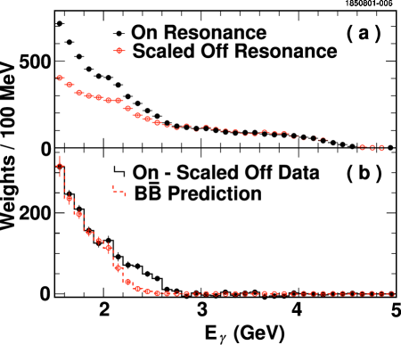
FIG. 1.: Photon energy spectra (weights per 100 MeV). The upper plot (a) shows the On $\Upsilon(4S)$ and scaled Off-resonance spectra. The lower plot (b) shows their difference, and the spectrum estimated for $B$ decay processes other than $b\rightarrow s\gamma$ and $b\rightarrow d\gamma$.

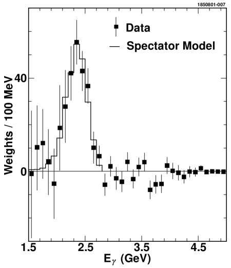
FIG. 2.: Observed laboratory frame photon energy spectrum (weights per 100 MeV) for On minus scaled Off minus $B$ backgrounds, the putative $b\rightarrow s\gamma$ plus $b\rightarrow d\gamma$ signal. No corrections have been applied for resolution or efficiency. Also shown is the spectrum from Monte Carlo simulation of the Ali-Greub spectator model with parameters $\langle m_{b}\rangle$ = 4.690 GeV, $P_{F}$ = 410 MeV/c, a good fit to the data.

REFERENCES

- [1] K. Adel and Y. P. Yao, Phys. Rev. D 49, 4945 (1994); C. Greub and T. Hurth, Phys. Rev. D 56, 2934 (1997); A. Ali and C. Greub, Phys. Lett. B 361, 146 (1995); C. Greub, T. Hurth, and D. Wyler, Phys. Lett. B 380, 385 (1996); Phys. Rev. D 54, 3350 (1996); A. Czarnecki and W. J. Marciano, Phys. Rev. Lett. 81, 277 (1998).
- [2] K. Chetyrkin, M. Misiak, and M. Münz, Phys. Lett. B 400, 206 (1997).
- [3] A. L. Kagan and M. Neubert, Eur. Phys. J. C 7, 5 (1999).
- [4] P. Gambino and M. Misiak, hep-ph/0104034.
- [5] SPIRES lists over 500 citations to our earlier branching fraction paper (ref.[9]), most of them theory papers addressing beyond-SM issues.
- [6] D. Cronin-Hennessy et al. (CLEO), CLEO 01-17, CLNS 01/1752, submitted to Phys. Rev. Lett.
- [7] M. Neubert, Phys. Rev D 49, 4623 (1994); A. K. Leibovich, I. Low, and I. Z. Rothstein, Phys. Rev. D 61, 053006 (2000).
- [8] F. De Fazio and M. Neubert, JHEP06, 017 (1999).
- [9] M. S. Alam et al. (CLEO), Phys. Rev. Lett. 74, 2885 (1995).
- [10] Z. Ligeti, M. Luke, A. V. Manohar, and M. B. Wise, Phys. Rev. D 60 034019, (1999); C. Bauer, Phys. Rev. D 57, 5611. (1998).
- [11] Adam Falk and Zoltan Ligeti, private communications.
- [12] Y. Kubota et al. (CLEO), Nucl. Instrum. Meth. A 320, 66 (1992).
- [13] T. Hill, Nucl. Instrum. Methods Phys. Res., Sect. A 418, 32 (1998).
- [14] Jana Thayer, Ph.D. thesis, Ohio State University (in progress).
- [15] G. Fox and S. Wolfram, Phys. Rev. Lett. 41, 1581 (1978).
- [16] J. A. Ernst, Ph.D. thesis, Univ. of Rochester (1995).
- [17] A. Ali and C. Greub, Phys. Lett. B 259, 182 (1991); and private communications.
- [18] D. E. Groom et al. (PDG), Eur. Phys. J. C 15, 1 (2000).
- [19] M. Neubert, hep-ph/9809377.