[hep-ex/0107076] A Study of the Lorentz Structure in Tau Decays

CERN–EP-2000-027

14 February 2000

DELPHI Collaboration

Abstract

This paper describes a measurement of the Michel parameters, $\eta$ , $\rho$ , $\xi$ , $\xi\delta$ , and the average $\nu_{\tau}$ helicity, $h_{\nu_{\tau}}$ , in $\tau$ lepton decays together with the first measurement of the tensor coupling in the weak charged current. The $\tau^{+}\tau^{-}$ pairs were produced at the LEP $\mathrm{e^{+}e^{-}}$ collider at CERN from 1992 through 1995 in the DELPHI detector. Assuming lepton universality in the decays of the $\tau$ the measured values of the parameters were: $\eta=-0.005\pm 0.036\pm 0.037$ , $\rho=0.775\pm 0.023\pm 0.020$ , $\xi=0.929\pm 0.070\pm 0.030$ , $\xi\delta=0.779\pm 0.070\pm 0.028$ , $h_{\nu_{\tau}}=-0.997\pm 0.027\pm 0.011$ . The strength of the tensor coupling was measured to be $\kappa^{W}_{\tau}=-0.029\pm 0.036\pm 0.018$ . The first error is statistical and the second error is systematic in all cases. The results are consistent with the $V\!-\!A$ structure of the weak charged current in decays of the $\tau$ lepton.

(Eur. Phys. J. C16(2000)229)

1 Introduction

The Michel parameters [1], $\eta$ , $\rho$ , $\xi$ , and $\xi\delta$ , are a set of experimentally accessible parameters which are bilinear combinations of ten complex coupling constants describing the couplings in the charged current decay of charged leptons. The Standard Model makes a specific prediction about the exact nature of the structure of the weak charged current. $\tau$ leptons provide a unique environment in which to verify this prediction. Not only is the large mass of the $\tau$ lepton (and thus an extensive range of decay channels) strong motivation to search for deviations from the Standard Model but the $\tau$ also offers the possibility to test the hypothesis of lepton universality.

The Michel parameters in $\tau$ decays have been extensively studied by many experiments both at $\mathrm{e^{+}e^{-}}$ colliders running at the $Z$ pole and at low energy machines [2, 3] This paper describes an analysis of $\tau$ decays using both the purely leptonic and the semi-leptonic (hadronic) decay modes, the latter being selected without any attempt to identify the specific decay channel. By grouping together all the semi-leptonic decays one can obtain a high efficiency and purity at the expense of a loss of sensitivity to the relevant parameters. This sensitivity is recuperated by splitting the semi-leptonic decay candidates into bins of invariant mass of the hadronic decay products, each bin being separately dominated by a different $\tau$ decay mode. Results are presented both with and without the assumption of lepton universality.

The measurement of the Michel parameters in the purely leptonic decay modes of the $\tau$ allows limits to be placed on new physics. The large number of Michel parameters, however, reduces the experimental sensitivity in placing these limits. Moreover, the Michel parameterisation does not cover the full variety of possible interactions; in particular it does not include terms with derivatives. However, a complementary test of a special type of new interaction is presented. In addition to testing new couplings with leptonic currents that conserve fermion chiralities, the possibility of an anomalous coupling of a leptonic charged tensor current is explored.

2 The Michel parameters and $\nu_{\tau}$ helicity

The most general, lepton-number conserving, derivative free, local, Lorentz invariant four-lepton interaction matrix element, $\cal{M}$ , describing the leptonic decay $\tau\rightarrow l\overline{\nu}_{l}\nu_{\tau}$ , ( $l=$ e or $\mu$ ), can be written as follows [4, 5, 6]:

\displaystyle\cal{M}

\displaystyle=

\displaystyle\frac{4G}{\sqrt{2}}\sum_{N=S,V,T\atop{i,j=L,R}}g^{N}_{ij}\left\langle\overline{v}_{l_{i}}\left|\;\Gamma^{N}\;\right|\left(v_{\overline{\nu}_{l}}\right)_{n}\right\rangle\left\langle(\overline{v}_{\nu_{\tau}})_{m}\left|\;\Gamma_{N}\;\right|u_{\tau_{j}}\right\rangle,

(1)

which is characterised by spinors of definite chirality. $G$ is a coupling constant, and the $\Gamma_{N}$ represent the various forms of the weak charged current allowed by Lorentz invariance. The $n$ and $m$ in Eqn. 1 are the chiralities of the neutrinos which are uniquely determined by a given $N$ , $i$ and $j$ . In the case of vector and axial-vector interactions the chirality of the neutrino is equal to the chirality of its associated charged lepton, while it is the opposite in the case of scalar, pseudoscalar and tensor interactions. In all cases we refer to the helicities and chiralities of particles; those of antiparticles are implicitly taken to have the opposite sign.

The $g^{N}_{ij}$ parameters are complex coupling constants. There are 12 of these but, excluding the possibility of the existence of a vector boson carrying a chiral charge, two of the constants, $g^{T}_{LL}$ and $g^{T}_{RR}$ , are identically zero. As the couplings can be complex, with an arbitrary phase, there are 19 independent parameters. The Standard Model $V\!-\!A$ structure for the weak charged current predicts that $g^{V}_{LL}=1$ with all other couplings being identically zero. Neglecting phase space effects, the rate for the decay $\tau^{-}\to l^{-}\nu_{\tau}\bar{\nu}_{l}$ can be written [7, 8] as

\Gamma(\tau^{-}\to l^{-}\nu_{\tau}\bar{\nu}_{l})=\frac{G^{2}m_{\tau}^{5}}{192\pi^{3}}\cdot\frac{A}{16},

(2)

with the definition

	$\displaystyle A$	$\displaystyle\equiv$	$\displaystyle 4\bigr{(}\|g^{S}_{RR}\|^{2}+\|g^{S}_{LR}\|^{2}+\|g^{S}_{RL}\|^{2}+\|g^{S}_{LL}\|^{2}\bigl{)}+48\bigr{(}\|g^{T}_{LR}\|^{2}+\|g^{T}_{RL}\|^{2}\bigl{)}$		(3)
			$\displaystyle+16\bigr{(}\|g^{V}_{RR}\|^{2}+\|g^{V}_{LR}\|^{2}+\|g^{V}_{RL}\|^{2}+\|g^{V}_{LL}\|^{2}\bigl{)}\hskip 11.38109pt\equiv\hskip 11.38109pt16.$		(3)

From the above normalisation condition the maximum values that the coupling constants $g^{N}_{ij}$ can take are 2, 1 and 1/ $\sqrt{3}$ for $N=S,V$ and $T$ respectively. The parameter $G$ has to be measured from the decay rate and absorbs any deviation in the overall normalisation. The shapes of the spectra and the ratios of branching ratios, as used in this analysis, are insensitive to the overall normalisation and hence to $G$ .

The matrix element written in Eqn. 1 can be used to form the decay distribution of the leptonic $\tau$ decay as follows:

	$\displaystyle\frac{1}{\Gamma}\frac{d\Gamma}{dx_{l}}$	$\displaystyle=$	$\displaystyle H_{0}(x_{l})-{\cal P}_{\tau}H_{1}(x_{l})$		(4)
		$\displaystyle=$	$\displaystyle[h_{0}(x_{l})+\eta h_{\eta}(x_{l})+\rho h_{\rho}(x_{l})]-{\cal P}_{\tau}[\xi h_{\xi}(x_{l})+\xi\delta h_{\xi\delta}(x_{l})]$		(5)

where $x_{l}=E_{l}/E_{max}$ is the normalised energy of the daughter lepton and ${\cal P}_{\tau}$ is the average $\tau$ polarisation. $E_{max}$ is the maximum kinematically allowed energy of the lepton, $l$ . In the rest frame of the $\tau$ , $E_{max}=\frac{m_{\tau}^{2}+m_{l}^{2}}{2m_{\tau}}$ . In the laboratory frame $E_{max}\approx E_{\tau}$ or the beam energy $E_{beam}$ . The $h$ ’s at Born level are polynomials and are illustrated in Fig. 1. The Michel parameters, $\eta$ , $\rho$ , $\xi$ and $\xi\delta$ , are bilinear combinations of the complex coupling constants [1] and take the following form in terms of the complex coupling constants:

$\displaystyle\eta$	$\displaystyle=$	$\displaystyle\textstyle\frac{1}{2}\mbox{Re}\left(6g^{V}_{LR}g^{T\ast}_{LR}+6g^{V}_{RL}g^{T\ast}_{RL}+g^{S}_{RR}g^{V\ast}_{LL}+g^{S}_{RL}g^{V\ast}_{LR}+g^{S}_{LR}g^{V\ast}_{RL}+g^{S}_{LL}g^{V\ast}_{RR}\right);$	(6)
$\displaystyle\rho$	$\displaystyle=$	$\displaystyle\textstyle\frac{3}{16}(4\|g^{V}_{LL}\|^{2}+4\|g^{V}_{RR}\|^{2}+\|g^{S}_{LL}\|^{2}+\|g^{S}_{RR}\|^{2}+\|g^{S}_{RL}-2g^{T}_{RL}\|^{2}+\|g^{S}_{LR}-2g^{T}_{LR}\|^{2});$	(7)
$\displaystyle\xi$	$\displaystyle=$	$\displaystyle-\textstyle\frac{1}{4}\bigr{(}\|g^{S}_{RR}\|^{2}+\|g^{S}_{LR}\|^{2}-\|g^{S}_{RL}\|^{2}-\|g^{S}_{LL}\|^{2}\bigl{)}~{}+~{}5\bigr{(}\|g^{T}_{LR}\|^{2}-\|g^{T}_{RL}\|^{2}\bigl{)}$	(8)
		$\displaystyle-\bigr{(}\|g^{V}_{RR}\|^{2}-3\|g^{V}_{LR}\|^{2}+3\|g^{V}_{RL}\|^{2}-\|g^{V}_{LL}\|^{2}\bigl{)}~{}+~{}4\mbox{Re}\bigr{(}g^{S}_{RL}g^{T\ast}_{RL}-g^{S}_{LR}g^{T\ast}_{LR}\bigl{)};$	(8)
$\displaystyle\xi\delta$	$\displaystyle=$	$\displaystyle\textstyle\frac{3}{16}(4\|g^{V}_{LL}\|^{2}-4\|g^{V}_{RR}\|^{2}+\|g^{S}_{LL}\|^{2}-\|g^{S}_{RR}\|^{2}+\|g^{S}_{RL}-2g^{T}_{RL}\|^{2}-\|g^{S}_{LR}-2g^{T}_{LR}\|^{2}).$	(9)

With the Standard Model predictions for these coupling constants the Michel parameters $\eta$ , $\rho$ , $\xi$ and $\xi\delta$ take on the values $𝟎$ , $\frac{3}{4}$ , $1$ and $\frac{3}{4}$ respectively.

Figure 1: Polynomial functions in the laboratory frame for the

\tau\rightarrow l\overline{\nu}_{l}\nu_{\tau}

decay channel at Born level. The

\eta

polynomial is normalised to

m_{\mu}/m_{\tau}

It is instructive to consider the physical significance of some of these parameters. A single measurement of $\rho$ does not constrain the form of the interaction. For example, if $\rho$ were to be measured to be $\frac{3}{4}$ , as is the case for the Standard Model prediction, then this would not rule out any combination of the six couplings $g^{S}_{LL},\,g^{S}_{LR},\,g^{S}_{RL},\,g^{S}_{RR},\,g^{V}_{RR},\,g^{V}_{LL}$ with the other couplings being zero. Indeed a $V\!+\!A$ structure would have a value of $\rho$ of $\frac{3}{4}$ . In this case one must examine the other parameters. For example, a $V\!+\!A$ structure would mean that the parameter $\xi$ would be equal to $-1$ . The values of the Michel parameters for several examples of interaction types are given in Table 1.

Vertices		Coupling	Parameters
$\tau-\nu_{\tau}$	$l-\nu_{l}$	Constants	$\rho$	$\delta$	$\xi$	$\eta$
V-A	V-A	$g^{V}_{LL}$ =1	$3/4$	$3/4$	1	0
V	V	$g^{V}_{LL}$ = $g^{V}_{RL}$ = $g^{V}_{LR}$ = $g^{V}_{RR}$ = $1/2$	$3/8$	$3/4$	0	0
A	A	$g^{V}_{LL}$ = $-g^{V}_{RL}$ = $-g^{V}_{LR}$ = $g^{V}_{RR}$ = $1/2$	$3/8$	$3/4$	0	0
V+A	V+A	$g^{V}_{RR}$ =1	$3/4$	$3/4$	-1	0
V	V-A	$g^{V}_{LL}$ = $g^{V}_{LR}$ = $1/\sqrt{2}$	$3/8$	$3/16$	2	0
A	V-A	$g^{V}_{LL}$ = $-g^{V}_{LR}$ = $1/\sqrt{2}$	$3/8$	$3/16$	2	0
V+A	V-A	$g^{V}_{LR}$ =1	0	0	3	0

Table 1: The couplings and Michel parameter values for various mixtures of vector and axial-vector coupling at the two vertices in the decay

\tau\rightarrow l\nu_{\tau}\overline{\nu}_{l}

The $\eta$ parameter is of particular interest. It is sensitive to the low energy part of the decay lepton spectrum. It is practically impossible to measure $\eta$ for $\tau\rightarrow\mathrm{e}\nu_{\tau}\overline{\nu}_{e}$ decays because of a heavily suppressive factor of $\frac{m_{e}}{m_{\tau}}$ in the $h_{\eta}$ polynomial. This suppressive factor is of the order of $\simeq 1/17$ for $\tau\rightarrow\mu\nu_{\tau}\overline{\nu}_{\mu}$ and hence all sensitivity to $\eta$ is in this channel. The $h_{\eta}$ polynomial receives contributions from the interference between vector and scalar and vector and tensor interactions and is therefore particularly sensitive to non $V\!-\!A$ interactions. If $\eta\neq 0$ there would be two or more different couplings with opposite chiralities for the charged leptons and this would result in non-maximal parity and charge conjugation violation. In this case, if $V\!-\!A$ is assumed to be dominant, then the second coupling could be a Higgs type coupling with a right handed $\tau$ and muon [7].

The leptonic decay rates of the $\tau$ lepton may be affected by the exchange of these non-standard charged scalar particles [9] and these effects can be conveniently expressed through the parameter $\eta$ [10, 11]. The generalised leptonic decay rate of the $\tau$ becomes

\displaystyle\Gamma(\tau\rightarrow l\nu_{\tau}\overline{\nu}_{l})=\frac{G_{l\tau}^{2}m_{\tau}^{5}}{192\pi^{3}}\left[f(\frac{m_{l}^{2}}{m_{\tau}^{2}})+4\frac{m_{l}}{m_{\tau}}g(\frac{m_{l}^{2}}{m_{\tau}^{2}})\eta\right]r_{RC}^{\tau}

(10)

where $G_{l\tau}$ is the coupling of the $\tau$ to a lepton of type $l$ , and equals the Fermi coupling constant if lepton universality holds. The functions $f$ and $g$ and the quantity $r_{RC}^{\tau}$ are described in [11]. The parameter $r_{RC}^{\tau}$ is a factor due to electroweak radiative corrections, which to a good approximation has the value $0.9960$ for both leptonic decay modes of the $\tau$ . The functions $f$ and $g$ are phase space factors. The factor $f(\frac{m_{{l}}^{2}}{m_{\tau}^{2}})$ is equal to $1.0000$ for electrons and $0.9726$ for muons. However, the function $4\frac{m_{{\rm e}}}{m_{\tau}}g(\frac{m_{{\rm e}}^{2}}{m_{\tau}^{2}})$ equals $0.0012$ , whereas the value of $4\frac{m_{\mu}}{m_{\tau}}g(\frac{m_{\mu}^{2}}{m_{\tau}^{2}})$ is relatively large, equal to $0.2168$ . Hence, under the assumption of lepton universality, a stringent limit on $\eta$ in $\tau\to\mu\overline{\nu}_{\mu}\nu_{\tau}$ decays can be set on the basis of the branching ratio measurements, since to a good approximation (see discussion in section 7),

\displaystyle\frac{Br(\tau\rightarrow\mu\nu_{\tau}\overline{\nu}_{\mu})}{Br(\tau\rightarrow\mathrm{e}\nu_{\tau}\overline{\nu}_{e})}

\displaystyle=

\displaystyle f\biggl{(}\frac{m_{\mu}^{2}}{m_{\tau}^{2}}\biggr{)}+4\frac{m_{\mu}}{m_{\tau}}g\biggl{(}\frac{m_{\mu}^{2}}{m_{\tau}^{2}}\biggr{)}\eta_{\mu}.

(11)

The variable $P^{\tau}_{R}$ is defined as the probability that a right handed $\tau$ will decay into a lepton of either handedness [7]. This variable is related to the Michel parameters $\xi$ and $\xi\delta$ and to five of the complex coupling constants in the following way:

	$\displaystyle\hskip 28.45274ptP^{\tau}_{R}\hskip 8.53581pt$	$\displaystyle=$	$\displaystyle\textstyle\frac{1}{4}\|g^{S}_{RR}\|^{2}+\textstyle\frac{1}{4}\|g^{S}_{LR}\|^{2}+\|g^{V}_{RR}\|^{2}+\|g^{V}_{LR}\|^{2}+3\|g^{T}_{LR}\|^{2}$		(12)
		$\displaystyle=$	$\displaystyle\textstyle\frac{1}{2}[1+\textstyle\frac{1}{3}\xi-\textstyle\frac{16}{9}\xi\delta].$		(12)

Hence the quantity $P^{\tau}_{R}$ is a measure of the contributions of five coupling constants involving right handed $\tau$ ’s. One can therefore see that measuring the parameters $\xi$ and $\xi\delta$ is of considerable interest in studying the structure of the weak charged currents.

The Michel parameters are restricted by boundary conditions. The leptonic decay rate of the $\tau$ in Eqn. 4 has to be positive definite. Certain combinations of the Michel parameters lead to unphysical effects. It has been shown [12, 13, 14] that the following constraints must be satisfied:

$\displaystyle 0\leq$	$\displaystyle\rho$	$\displaystyle\leq 1,$	(13)
$\displaystyle\|\xi\|$	$\displaystyle\leq$	$\displaystyle 3,$	(14)
$\displaystyle\rho-\left\|\xi\delta\right\|$	$\displaystyle\geq$	$\displaystyle 0,$	(15)
$\displaystyle 9-9\rho+\left\|7\xi\delta-3\xi\right\|$	$\displaystyle\geq$	$\displaystyle 0.$	(16)

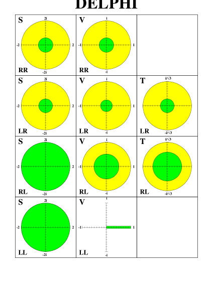
These inequalities describe the interior and surface of a tetrahedron in ( $\rho$ , $\xi$ , $\xi\delta$ ) space. The first two conditions arise from the fact that the different couplings in the definitions of the Michel parameters occur in quadrature. The 3rd constraint can be found directly if the $\tau$ decay rate in Eqn. 4 is forced to be positive definite for all values of $x_{l}$ . The 4th constraint is derived from the equations of two of the surfaces of the physically allowed tetrahedron. It is interesting to note that the Standard Model values of the Michel parameters are consistently at the edge of the allowed region (see Fig. 9). These relations are used in Section 9 to place limits on the coupling constants using the measured values of the Michel parameters.

The decay width of the semi-leptonic decays of the $\tau$ can be written, assuming vector and axial-vector couplings at the decay vertices as

	$\displaystyle\frac{1}{\Gamma}\frac{d\Gamma}{dx}$	$\displaystyle=$	$\displaystyle H_{0}(x)+{\cal P}_{\tau}H_{1}(x)$		(17)
		$\displaystyle=$	$\displaystyle H_{0}(x)-h_{\nu_{\tau}}{\cal P}_{\tau}H_{1}(x)$		(17)

where $x$ is a polarisation sensitive variable in each decay channel. For the case of $\tau\rightarrow\pi\nu_{\tau}$ this variable is $\cos\theta^{*}$ , the decay angle of the $\pi$ in the $\tau$ rest frame, whilst for the two cases of $\tau\rightarrow\rho\nu_{\tau}$ and $\tau\rightarrow a_{1}\nu_{\tau}$ the variable used is the $\omega$ variable described in [15]. The polarisation parameter $h_{\nu_{\tau}}$ is defined as

h_{\nu_{\tau}}=\frac{2{\rm Re}(v_{\tau}a_{\tau}^{*})}{\left|v_{\tau}\right|^{2}+\left|a_{\tau}\right|^{2}},

(18)

where $v_{\tau}$ and $a_{\tau}$ are the vector and axial-vector couplings of the $\tau$ lepton to $W$ bosons. In the limit of a massless $\nu_{\tau}$ this is equivalent to the $\tau$ neutrino helicity.

Assuming that the boson exchanged in producing the $\tau^{+}\tau^{-}$ pair only involves vector and axial-vector type couplings then the helicities of the $\tau^{+}$ and $\tau^{-}$ are almost 100% anti-correlated. This fact is used to construct the correlated spectra:

	$\displaystyle\frac{1}{\Gamma}\frac{d^{2}\Gamma}{dx_{1}dx_{2}}$	$\displaystyle=$	$\displaystyle\frac{1+{\cal P}_{\tau}}{2}\left(H_{0}(x_{1})-H_{1}(x_{1})\right)\left(H_{0}(x_{2})-H_{1}(x_{2})\right)+$		(19)
			$\displaystyle\frac{1-{\cal P}_{\tau}}{2}\left(H_{0}(x_{1})+H_{1}(x_{1})\right)\left(H_{0}(x_{2})+H_{1}(x_{2})\right)$		(19)

in terms of the polarisation sensitive variable $x$ (which is decay channel dependent). For leptonic decays the $H_{0}$ and $H_{1}$ functions are the polynomials described previously in Eqns. 4 and 17 and the polarisation sensitive variable is the scaled energy $x_{l}$ .

It follows therefore that by performing two-dimensional fits over this distribution one has full experimental access to all of the Michel parameters together with the $\tau$ neutrino helicity, $h_{\nu_{\tau}}$ , and the $\tau$ polarisation, ${\cal P}_{\tau}$ , with the caveat that only vector and axial-vector currents are assumed to contribute in the semileptonic decays.

3 Anomalous tensor couplings

The Lagrangian for the decay of the $\tau$ can be written in the following way:

{\cal L}=\frac{g}{\sqrt{2}}~{}W^{\alpha}~{}\left\{\overline{\tau}\gamma_{\alpha}\frac{1-\gamma^{5}}{2}\nu+\frac{\kappa^{W}_{\tau}}{2m_{\tau}}\partial_{\beta}\left(\overline{\tau}\sigma_{\alpha\beta}\frac{1-\gamma^{5}}{2}\nu\right)\right\}+{\mathrm{h}.c.}

(20)

where $W^{\alpha}$ is the weak charged current of the decay products of the W boson and $\kappa^{W}_{\tau}$ is a parameter which controls the strength of the tensor coupling. The choice of such a kind of interaction to test for the existence of new physics is inspired by experiments with semi-leptonic decays of pions [16] and kaons [17], which show a deviation from the Standard Model which can be explained by the existence of an anomalous interaction with a tensor leptonic current [18]. Since the new interaction explicitly contains derivatives, its effect on the distortion of the energy spectrum of charged leptons in $\tau$ decays can not be described in terms of the known Michel parameters. Constraints will be placed on the parameter $\kappa^{W}_{\tau}$ from the analysis of both leptonic and semi-leptonic $\tau$ decays, fixing the Michel parameters to their Standard Model values. The inclusion of the semi-leptonic channels significantly increases the sensitivity to the new tensor coupling and imposes stricter constraints.

For purely leptonic decays, the matrix element takes the form

\displaystyle\cal{M}

\displaystyle=

\displaystyle\frac{4G}{\sqrt{2}}\langle\overline{v}_{l}\left|\;\gamma_{\alpha}\right|v_{\overline{\nu}_{l}}\rangle\left(\langle\overline{v}_{\nu_{\tau}}\left|\;\gamma_{\alpha}\right|u_{\tau_{L}}\rangle-i\frac{\kappa^{W}_{\tau}}{2m_{\tau}}q_{\beta}\langle\overline{v}_{\nu_{\tau}}\left|\;\sigma_{\alpha\beta}\right|u_{\tau_{R}}\rangle\right),

(21)

where $q$ is the momentum of the $W$ . The laboratory energy spectrum of the charged decay product can be expressed as

\frac{{\rm d}\Gamma}{{\rm d}x_{l}}\propto f(x_{l})+{\cal P}_{\tau}g(x_{l}),

(22)

where $x_{l}$ is again the normalised energy of the daughter lepton as defined in section 2.

The expressions for $f(x_{l})$ and $g(x_{l})$ , accounting for the new tensor interaction, were obtained in the rest frame of a decaying lepton [19]. Neglecting the mass of the final lepton and boosting along the $\tau$ flight direction gives

	$\displaystyle f(x_{l})$	$\displaystyle=$	$\displaystyle~{}5-9x_{l}^{2}+4x_{l}^{3}+2\kappa^{W}_{\tau}(1-x_{l}^{3}),$
	$\displaystyle g(x_{l})$	$\displaystyle=$	$\displaystyle~{}1-9x_{l}^{2}+8x_{l}^{3}+2\kappa^{W}_{\tau}(1-3x_{l}+2x_{l}^{3}).$		(23)

These functions are shown in Fig. 2.

Figure 2: Polynomial functions for the tensor coupling contribution in the

\tau\rightarrow l\overline{\nu}_{l}\nu_{\tau}

decay channel at Born level. Left plot shows

f(x_{l})

and right plot shows

g(x_{l})

. In both plots the solid line illustrates the Standard Model case,

\kappa^{W}_{\tau}=0

, and the dashed line the case for

\kappa^{W}_{\tau}=1

In the Born approximation the tensor interaction does not contribute to the process $\tau\rightarrow\pi\nu_{\tau}$ . Thus, among the main $\tau$ semi-leptonic decay modes, only the decay modes $\tau\rightarrow\rho\nu_{\tau}\rightarrow(2\pi)\nu_{\tau}$ and $\tau\rightarrow a_{1}\nu_{\tau}\rightarrow(3\pi)\nu_{\tau}$ yield information about the new tensor interaction. The sensitivity can be increased by performing the analysis using the two angular variables $\theta^{*}$ and $\psi$ , where $\theta^{*}$ is the angle between the emitted final (pseudo) vector particle after a Lorentz transformation into the $\tau$ rest frame and the inverse of the three-vector component of this Lorentz transformation. The angle $\psi$ is related to the angle of the $\rho$ or $a_{1}$ decay products in the $\rho$ or $a_{1}$ system and is sensitive to the polarisation of the hadronic system. These two variables are discussed in [15].

The $\tau$ decay to a particle of spin 1 and mass $m_{h}$ and a neutrino has two amplitudes, $A_{L}$ and $A_{T}$ , representing longitudinal and transverse polarisation of the spin-1 particle respectively. From the expression for the decay helicity amplitudes,

{\cal M}_{\lambda}\propto\overline{v}_{\overline{\nu}_{l}}(1+\gamma^{5})\left[\gamma_{\alpha}-i\frac{\kappa^{W}_{\tau}}{2m_{\tau}}q_{\beta}\sigma_{\alpha\beta}\right]u_{\tau}~{}\epsilon^{*}_{\alpha}(q,\lambda),

(24)

where $\epsilon^{*}_{\alpha}$ is the polarisation vector of the spin 1 particle with momentum $q$ and helicity $\lambda$ , one obtains

\frac{A_{T}}{A_{L}}=\frac{\sqrt{2}m_{h}}{m_{\tau}}~{}\frac{a_{T}}{a_{L}},

(25)

where $a_{T}=1+\kappa^{W}_{\tau}/2$ and $a_{L}=1+(m^{2}_{h}/m^{2}_{\tau})\kappa^{W}_{\tau}/2$ . Therefore for $\tau\rightarrow(2\pi)~{}\nu$ and $\tau\rightarrow(3\pi)~{}\nu$ ,

\frac{{\rm d}^{2}N}{{\rm d}\cos{\theta^{*}}~{}{\rm d}\cos{\psi}}\propto(1+{\cal P}_{\tau})H^{+}+(1-{\cal P}_{\tau})H^{-},

(26)

where

$\displaystyle H^{+}$	$\displaystyle=$	$\displaystyle~{}h_{0}(\psi)\left(a_{L}m_{\tau}\cos{\eta}\cos{\textstyle\frac{\theta^{}}{2}}+a_{T}m_{h}\sin{\eta}\sin{\textstyle\frac{\theta^{}}{2}}\right)^{2}$	(27)
	$\displaystyle+$	$\displaystyle~{}h_{1}(\psi)\left[\left(a_{L}m_{\tau}\sin{\eta}\cos{\textstyle\frac{\theta^{}}{2}}-a_{T}m_{h}\cos{\eta}\sin{\textstyle\frac{\theta^{}}{2}}\right)^{2}+a^{2}_{T}m^{2}_{h}\sin^{2}\textstyle\frac{\theta^{*}}{2}\right],$	(27)
$\displaystyle H^{-}$	$\displaystyle=$	$\displaystyle~{}h_{0}(\psi)\left(a_{L}m_{\tau}\cos{\eta}\sin{\textstyle\frac{\theta^{}}{2}}-a_{T}m_{h}\sin{\eta}\cos{\textstyle\frac{\theta^{}}{2}}\right)^{2}$	(28)
	$\displaystyle+$	$\displaystyle~{}h_{1}(\psi)\left[\left(a_{L}m_{\tau}\sin{\eta}\sin{\textstyle\frac{\theta^{}}{2}}+a_{T}m_{h}\cos{\eta}\cos{\textstyle\frac{\theta^{}}{2}}\right)^{2}+a^{2}_{T}m^{2}_{h}\cos^{2}\textstyle\frac{\theta^{*}}{2}\right],$	(28)

and

h_{0}(\psi)=\left\{\begin{array}[]{l}2\cos^{2}\psi\\ \sin^{2}\psi\end{array}\right.\begin{array}[t]{l}h_{1}(\psi)=\\ \end{array}\left\{\begin{array}[]{l}2\sin^{2}\psi\\ (1+\cos^{2}\psi)/2\end{array}\right.\begin{array}[t]{l}\mbox{for}\\ \end{array}\left\{\begin{array}[]{l}\tau^{-}\rightarrow(2\pi)~{}\nu_{\tau}\\ \tau^{-}\rightarrow(3\pi)~{}\nu_{\tau}\end{array}\right..

Note that the angle $\eta$ used here is unrelated to to the Michel parameter of the same name. Neglecting terms of ${\cal O}(m^{2}_{\tau}/E_{\tau}^{2})$ , the relation between $\eta$ and $\theta^{*}$ is

\cos{\eta}=\frac{m_{\tau}^{2}-m^{2}_{h}+(m_{\tau}^{2}+m^{2}_{h})\cos{\theta^{*}}}{m_{\tau}^{2}+m^{2}_{h}+(m_{\tau}^{2}-m^{2}_{h})\cos{\theta^{*}}}.

(29)

4 The DELPHI Detector

The DELPHI detector is described in detail elsewhere [20, 21]. The following is a summary of the subdetector units particularly relevant for this analysis. All these covered the full solid angle of the analysis except where specified. In the DELPHI reference frame the z-axis is taken along the direction of the e^- beam. The angle $\Theta$ is the polar angle defined with respect to the z-axis, $\phi$ is the azimuthal angle about this axis and $r$ is the distance from this axis. The reconstruction of a charged particle trajectory in the barrel region of DELPHI resulted from a combination of the measurements in:

•

the Vertex Detector (VD), made of three layers of silicon micro-strip modules, at radii of 6.3, 9.0 and 11.0 cm from the beam axis. The space point precision in r- $\phi$ was about $8~{}\mu$ m, while the two track resolution was 100 $\mu$ m. For the 1994 and 1995 data the innermost and outermost layers of the VD were equipped with double sided silicon modules, giving two additional measurements of the z coordinate.
•

the Inner Detector (ID), with an inner radius of 12 cm and an outer radius of 28 cm. A jet chamber measured 24 r- $\phi$ coordinates and provided track reconstruction. Its two track resolution in r- $\phi$ was 1 mm and its spatial precision $40~{}\mu$ m. It was surrounded by an outer part which served mainly for triggering purposes. This outer part was replaced for the 1995 data with a straw-tube detector containing much less material.
•

the Time Projection Chamber (TPC), extending from 30 cm to 122 cm in radius. This was the main detector for the track reconstruction. It provided up to 16 space points for pattern recognition and ionisation information extracted from 192 wires. Every $60^{\circ}$ in $\phi$ there was a boundary region between read-out sectors about $1^{\circ}$ wide which had no instrumentation. At cos $\Theta=0$ there was a cathode plane which caused a reduced tracking efficiency in the polar angle range $|$ cos $\Theta|\!<\!0.035$ . The TPC had a two track resolution of about 1.5 cm in r- $\phi$ and in z. The measurement of the ionisation deposition had a typical precision of $\pm 6\%$ .
•

the Outer Detector (OD) with 5 layers of drift cells at a radius of 2 m from the beam axis, sandwiched between the RICH and HPC sub-detectors described below. Each layer provided a space point with 110 $\mu$ m precision in r- $\phi$ and about 5 cm precision in z.

These detectors were surrounded by a solenoidal magnet with a 1.2 Tesla field parallel to the z-axis. In addition to the detectors mentioned above, the identification of the $\tau$ decay products relied on:

•

the barrel electromagnetic calorimeter, a High density Projection Chamber (HPC). This detector lay immediately outside the tracking detectors and inside the magnet coil. Eighteen radiation lengths deep for perpendicular incidence, its energy resolution was $\Delta E/E=0.31/E^{0.44}\oplus 0.027$ where $E$ is in units of GeV. It had a high granularity and provided a sampling of shower energies from nine layers in depth. It allowed a determination of the starting point of an electromagnetic shower with an accuracy of 0.6 mrad in polar angle and 3.1 mrad in azimuthal angle. The HPC had a modularity of $15^{\circ}$ in azimuthal angle. Between modules there was a region with a width of about $1^{\circ}$ in azimuth where the energy resolution was degraded. The HPC lay behind the OD and the Ring Imaging CHerenkov detector (RICH), not used in this analysis, which contained about 60% of a radiation length.
•

the Hadron CALorimeter (HCAL), sensitive to hadronic showers and minimum ionising particles. It was segmented in 4 layers in depth, with a granularity of $3.75^{\circ}$ in polar angle and $2.96^{\circ}$ in azimuthal angle. Lying outside the magnet solenoid, it had a depth of 110 cm of iron.
•

the barrel muon chambers consisting of two layers of drift chambers, the first one situated after 90 cm of iron and the second outside the hadron calorimeter. The acceptance in polar angle of the outer layer was slightly smaller than the other barrel detectors and covered the range $|$ cos $\Theta|\!<\!0.602$ . The polar angle range $0.602\!<\!|$ cos $\Theta|$ was covered by the forward muon chambers in certain azimuthal zones.

The DELPHI trigger was very efficient for $\tau$ final states due to the redundancy existing between its different components. From the comparison of the response of independent components, a trigger efficiency of $(99.98\pm 0.01)\%$ has been derived.

5 Particle identification and energy calibration

The detector response was extensively studied using simulated data together with various test samples of real data where the identity of the particles was unambiguously known. Examples of such samples consisted of $\mathrm{e^{+}e^{-}\rightarrow e^{+}e^{-}}$ , and $\mathrm{e^{+}e^{-}}\rightarrow\mu^{+}\mu^{-}$ events together with the radiative processes $\mathrm{e^{+}e^{-}\rightarrow e^{+}e^{-}}\gamma$ and $\mathrm{e^{+}e^{-}}\rightarrow\mu^{+}\mu^{-}\gamma$ . Test samples using the redundancy of the detector were also used. An example of such a sample is $\tau\rightarrow\pi(n\pi^{0})$ , $(n>0)$ , selected by tagging the $\pi^{0}$ decay in the HPC. This sample was extensively used as a pure sample of charged hadrons to test the response of the calorimetry and muon chambers.

5.1 TPC ionisation measurement

The ionisation loss of a track as it travels through the TPC gives good separation between electrons and charged pions, particularly in the low momentum range. Because of the importance of this variable it was required that there were at least 28 anode wires used in the measurement. This reduced the sample by a small amount primarily due to particles being close to the boundary regions of the TPC sectors where a narrow non-instrumented strip was located. The $dE/dx$ pull variable, $\prod^{j}_{dE/dx}$ , for a particular particle hypothesis ( $j$ = e, $\mu$ , $\pi$ , $K$ ) is defined as

{\textstyle\prod^{j}_{dE/dx}}=\frac{{dE/dx}_{meas}-{dE/dx}_{expt}(j)}{\sigma(dE/dx)}

(30)

where ${dE/dx}_{meas}$ is the measured value, ${dE/dx}_{expt}(j)$ is the expected momentum dependent value for a hypothesis $j$ and $\sigma(dE/dx)$ is the resolution of the measurement.

5.2 Electromagnetic calorimetry

The HPC is used for $\mathrm{e},\gamma$ and $\pi^{0}$ identification. For charged particles $E_{ass}$ is the energy deposited in the HPC. For electrons this energy should be (within experimental errors) equal to the measured value of the momentum. Muons, being minimum ionising particles, deposit only a small amount of energy in the calorimeter. Most charged hadrons interact deep in the HPC or in the HCAL and thus look like a minimum ionising particle in the early part or all of the HPC, with an increased energy deposition in the later layers if an interaction occurs in the HPC.

The ratio of the energy deposition in the HPC to the reconstructed momentum has a peak at one for electrons and a rising distribution towards zero for hadrons. The pull variable, ${\textstyle\prod_{E/p}}$ , is defined as

{\textstyle\prod_{E/p}}=\frac{E_{ass}/p^{\prime}-1}{\sigma(E_{ass}/p^{\prime};E_{ass})}

(31)

where $p^{\prime}$ is the momentum refit without the use of the OD, described in Section 5.4 below, and $\sigma(E_{ass}/p^{\prime};E_{ass})$ is the expected resolution on $E_{ass}/p^{\prime}$ for an electron with associated energy $E_{ass}$ . This variable gives particularly good separation at high momenta.

5.3 Hadron calorimetry and muon identification

The HCAL was used in particular for separating pions from muons. As muons travel through the HCAL they deposit a small amount of energy evenly through the 4 layers and travel on into the muon chambers whereas hadrons deposit all their energy late in the HPC and/or in the first layers of the HCAL so that they rarely penetrate through to the muon chambers. Therefore muons can be separated from hadrons by demanding energy associated to the particle in the last layer of the HCAL together with an associated hit in the muon chambers. To further distinguish muons from hadrons one can construct the variable $E_{hlay}$ , the average energy deposited in the HCAL per HCAL layer defined as:

E_{hlay}=\frac{E_{HCAL}}{N_{layers}}\times\sin^{2}\Theta

(32)

where $E_{HCAL}$ is the total deposited energy in the HCAL; $N_{layers}$ is the number of HCAL layers with an energy deposit and $\sin^{2}\Theta$ smoothes out the angular dependence of the energy response of the HCAL (see Fig. 3). This variable can be seen in Fig. 3. Note that the step behaviour around polar angles of $50^{\circ}$ and $130^{\circ}$ is due to the reduction in the number of layers hit in the HCAL where a muon passes through a mixture of barrel geometry and end-cap geometry.

Figure 3: The HCAL response to muons (left plot) together with the variable

E_{hlay}

(right plot) for a sample of hadrons and muons in 1994 data (barrel region only). The crosses are the data, the solid histogram is the simulated sum of hadrons and muons and the hatched area is the simulated muons.

5.4 Momentum determination and scale

A good knowledge of the momentum and energy of charged particles is required for a Michel parameter analysis. This is especially true for the leptonic channels. As already mentioned the momentum is measured by tracking the particles in a magnetic field as they traverse the detector. The precision on the component of momentum transverse to the beam direction, $p_{t}$ , obtained with the DELPHI tracking detectors was $\Delta(1/p_{t})=0.0008\rm{(GeV/c)^{-1}}$ for particles (except electrons) with the same momentum as the beam. Calibration of the momentum is performed with $\mathrm{e^{+}e^{-}}\rightarrow\mu^{+}\mu^{-}$ events. For lower momenta the masses of the $K^{0}_{s}$ and the $J/\psi$ are reconstructed to give an absolute momentum scale for particles other than electrons estimated, to a precision of 0.2% over the full momentum range.

The determination of the momentum of electrons is more complicated. In passing through the RICH from the TPC to the OD, particles traverse about 60% of a radiation length. A large fraction of electrons therefore lose a substantial amount of energy through bremsstrahlung before they reach the OD. Due to this the standard momentum measurement of electrons would always tend to be biased to lower values. This effect is somewhat reduced through only using the measured momentum without using the OD, $p^{\prime}$ . The result is that this “refit momentum” shows a more Gaussian behaviour than the standard momentum fit. The best estimate for the momentum of the electron, $p_{el}$ , is constructed in such a way as to benefit from the better resolution of the momentum measurement at low momentum and the smaller bremsstrahlung bias of the electromagnetic energy measurement. The reconstructed momentum and the electromagnetic energy were combined through a weighted average which took into account the downward biases of the two respective measurements. The energy of the radiated photons was also added to the electromagnetic energy measurement to reduce further the effects of bremsstrahlung.

An algorithm was used which performed a weighted average depending on the value of $E_{ass}/p^{\prime}$ . The further this value was from unity, the more the weight of the estimator with the lower value was down scaled relative to the other. The scaling factor was inversely proportional to the square of the number of standard deviations by which the value of $E_{ass}/p^{\prime}$ differed from unity.

Subsequent references to the momenta of electrons imply the use of the best estimator $p_{el}$ . The momenta of other particles are measured using the standard momentum fit, $p$ , of the particle as it traverses the detector.

6 The selection of the event sample

In order to determine the Michel parameters, a sample of exclusively selected leptonic decays of the $\tau$ together with an inclusive sample of semi-leptonic decays have been used. The data sample corresponds to the data taken by DELPHI during 1992 (22.9 $pb^{-1}$ at $E_{cm}=$ 91.3 GeV), 1993 (15.7 $pb^{-1}$ at $E_{cm}=$ 91.2 GeV, 9.4 $pb^{-1}$ at $E_{cm}=$ 89.2 GeV and 4.5 $pb^{-1}$ at $E_{cm}=$ 93.2 GeV), 1994 (47.4 $pb^{-1}$ at $E_{cm}=$ 91.2 GeV) and 1995 (14.3 $pb^{-1}$ at $E_{cm}=$ 91.2 GeV, 9.2 $pb^{-1}$ at $E_{cm}=$ 89.2 GeV and 9.3 $pb^{-1}$ at $E_{cm}=$ 93.2 GeV).

In all analyses, samples of simulated events were used which had been passed through a detailed simulation of the detector response [21] and reconstructed with the same program as the real data. The Monte Carlo event generators used were: KORALZ 4.0 [22] together with the TAUOLA 2.5 [23] $\tau$ decay package for $\mathrm{e^{+}e^{-}}\rightarrow\tau^{+}\tau^{-}$ events; DYMU3 [25] for $\mathrm{e^{+}e^{-}}\rightarrow\mu^{+}\mu^{-}$ events; BABAMC [26] for $\mathrm{e^{+}e^{-}\rightarrow e^{+}e^{-}}$ events; JETSET 7.3 [27] for $\mathrm{e^{+}e^{-}}\rightarrow q\overline{q}$ events; Berends-Daverveldt-Kleiss [28] for $\mathrm{e^{+}e^{-}\rightarrow e^{+}e^{-}e^{+}e^{-}}$ , $\mathrm{e^{+}e^{-}\rightarrow e^{+}e^{-}}\mu^{+}\mu^{-}$ and $\mathrm{e^{+}e^{-}\rightarrow e^{+}e^{-}}\tau^{+}\tau^{-}$ events; TWOGAM [29] for $\mathrm{e^{+}e^{-}\rightarrow e^{+}e^{-}q\bar{q}}$ events.

The variables used in the initial preselection of the $\tau$ sample together with the selection of the various decay channels are described below.

6.1 The $\mathrm{e^{+}e^{-}}\rightarrow\tau^{+}\tau^{-}$ sample

At LEP energies, a $\tau^{+}\tau^{-}$ event appears as two highly collimated low multiplicity jets in approximately opposite directions. An event was separated into hemispheres by a plane perpendicular to the event thrust axis, where the thrust was calculated using all charged particles with momentum greater than 0.6 GeV/c. To be included in the sample, it was required that the highest momentum charged particle in at least one of the two hemispheres lie in the polar angle range $|\cos\Theta|<0.732$ .

Background from $\mathrm{e^{+}e^{-}}\rightarrow q\overline{q}$ events was reduced by requiring a charged particle multiplicity less than six and a minimum thrust value of 0.996. The $\mathrm{e^{+}e^{-}}\rightarrow q\overline{q}$ background is however negligible in the analysis of the Michel parameters as one is looking for events with only one charged particle in each hemisphere.

Cosmic rays and beam gas interactions were rejected by requiring that the highest momentum charged particle in each hemisphere have a point of closest approach to the interaction region less than 4.5 cm in $z$ and less than 1.5 cm in the $r-\phi$ plane. It was furthermore required that these particles have a difference in $z$ of their points of closest approach at the interaction region of less than 3 cm. The offset in $z$ of tracks in opposite hemispheres of the TPC was sensitive to the time of passage of a cosmic ray event with respect to the interaction time of the beams. The background left in the selected sample was computed from the data by interpolating the distributions outside the selected regions.

Two-photon events were removed by requiring a total energy in the event, $E_{vis}$ , greater than 8 GeV and a total transverse component of the vector sum of the charged particle momenta in the event, $p^{miss}_{t}$ , greater than 0.4 GeV/c.

Contamination from $\mathrm{e^{+}e^{-}\rightarrow e^{+}e^{-}}$ and $\mathrm{e^{+}e^{-}}\rightarrow\mu^{+}\mu^{-}$ events was reduced by requiring that the event acollinearity, $\theta_{acol}=\cos^{-1}(-\frac{p_{1}\cdot p_{2}}{|p_{1}||p_{2}|})$ , be greater than $0.5^{\circ}$ . The variables $p_{1}$ and $p_{2}$ are the momenta of the highest momenta charged particles in hemisphere 1 and 2 respectively.

The $\mathrm{e^{+}e^{-}\rightarrow e^{+}e^{-}}$ background is reduced in the second instance with a cut on the radial energy $E_{rad}$ (defined as $E_{rad}=\sqrt{{E_{1}}^{2}+{E_{2}}^{2}}/E_{beam}$ where $E_{1}$ and $E_{2}$ are the energies deposited in the HPC in a $30^{\circ}$ cone around the highest momentum charged particle in each hemisphere and $E_{beam}$ is the beam energy). Events are retained if $E_{rad}<1$ .

The $\mathrm{e^{+}e^{-}}\rightarrow\mu^{+}\mu^{-}$ background is reduced in the second instance with a cut on the radial momentum $p_{rad}$ (defined as $p_{rad}=\sqrt{{p_{1}}^{2}+{p_{2}}^{2}}/p_{beam}$ where $p_{1}$ and $p_{2}$ are the momenta of the highest momentum charged particles in each hemisphere and $p_{beam}$ is the beam momentum). Cutting on this quantity is also effective in reducing the $\mathrm{e^{+}e^{-}\rightarrow e^{+}e^{-}}$ background. Events are retained if $p_{rad}<1$ .

As a result of the above selection $\sim 93000$ $\mathrm{e^{+}e^{-}}\rightarrow\tau^{+}\tau^{-}$ candidates were selected from the 1992 to 1995 data set. The efficiency of selection in the $4\pi$ solid angle was $\sim 54\%$ . The background arising from $\mathrm{e^{+}e^{-}\rightarrow e^{+}e^{-}}$ events was estimated to be $(1.07\pm 0.32)\%$ , from $\mathrm{e^{+}e^{-}}\rightarrow\mu^{+}\mu^{-}$ events $(0.30\pm 0.09)\%$ and from four-fermion processes $(0.93\pm 0.28)\%$ . The background from $\mathrm{e^{+}e^{-}}\rightarrow\mathrm{e^{+}e^{-}q\bar{q}}$ was negligible. Since the efficiencies and backgrounds varied slightly from year to year the data sets were treated independently.

6.2 The $\tau\rightarrow\mathrm{e}\overline{\nu}_{e}\nu_{\tau}$ channel

The $\tau\rightarrow\mathrm{e}\overline{\nu}_{e}\nu_{\tau}$ decay has the signature of an isolated charged particle which produces an electromagnetic shower in the calorimetry. The produced electrons are ultra-relativistic and leave an ionisation deposition in the Time Projection Chamber corresponding to the plateau region above the relativistic rise. Backgrounds from other $\tau$ decays arise principally from one-prong hadronic decays where either the hadron interacts early in the electromagnetic calorimeter or an accompanying $\pi^{0}$ decay is wrongly associated to the charged particle track.

As an initial step in electron identification it was required that there be one charged particle in the hemisphere with a momentum greater than $0.01p_{beam}$ . To ensure optimal use of the HPC it was required that the track lie in the polar angle range $0.035<\left|\cos{\Theta}\right|<0.707$ and that the track extrapolation to the HPC should lie outside any HPC azimuthal boundary region, as described in Section 4.

The $dE/dx$ measurement is crucial to the analysis and so it was required that there were at least 28 anode wires with ionisation information in the TPC. It was required that the $dE/dx$ measurement be consistent with that of an electron by requiring that the ${\prod^{e}}_{dE/dx}$ variable be greater than -2. This requirement was efficient, especially at low momentum, in retaining signal and removing backgrounds from muons and hadrons.

The selection continued with a logical “OR” of two criteria, the first on the ${\prod^{\pi}}_{dE/dx}$ variable, which was particularly good at low momentum, and the second on the ${\prod}_{E/p}$ variable, which was particularly good at high momentum. A particle was taken to be an electron if it deposited greater than 0.5 GeV in the HPC and the value of ${\prod}_{E/p}$ was greater than -2 “OR” the measured value of ${\prod^{\pi}}_{dE/dx}$ was greater than 3 and the momentum was greater than 0.01 $p_{beam}$ . The “OR” thus gives a high constant efficiency over the whole momentum range. The ${\prod^{e}}_{dE/dx}$ and ${\prod}_{E/p}$ variables can be seen in Fig. 4.

Figure 4: The

{\prod^{e}}_{dE/dx}

and

{\prod}_{E/p}

variables after application of all the other selection cuts except the one shown for 1994 data. The crosses are the data, the solid histogram is the sum of the signal and background and the shaded area is the background from

\tau\not\rightarrow\mathrm{e}\nu\overline{\nu}

events.

The remaining background was reduced by requiring that there be no hits in the muon chambers and no deposited energy beyond the first HCAL layer. Residual background from $\tau\rightarrow\pi(n\pi^{0})\nu$ was reduced by cutting on the energy of the most energetic neutral shower in the HPC observed in an $18^{\circ}$ cone around the track. Neutral showers were not included in this requirement if they were within $1^{\circ}$ of the track and hence compatible with being bremsstrahlung photons.

The identification criteria were studied on test samples of real data. The efficiency of the $dE/dx$ and HPC cuts were tested across the whole momentum range by exploiting the redundancy of the two. Since the simulation showed that the two measurements were instrumentally uncorrelated, the overall bin by bin efficiency was calculated from these two independent measurements.

Backgrounds arising from non- $\tau$ sources consisted of $\mathrm{e^{+}e^{-}\rightarrow e^{+}e^{-}}$ and four-fermion $\mathrm{e^{+}e^{-}\rightarrow e^{+}e^{-}e^{+}e^{-}}$ events. The $\mathrm{e^{+}e^{-}\rightarrow e^{+}e^{-}}$ background was suppressed by the standard $\tau$ preselection cuts, i.e. $p_{rad}<1$ and $E_{rad}<1$ . Four-fermion events remaining after the $E_{vis}$ and $P_{t}^{miss}$ cuts were further suppressed by demanding that if the $\tau\rightarrow\mathrm{e}\nu_{\tau}\bar{\nu}_{\mathrm{e}}$ candidate had a momentum less than $0.2E_{beam}$ and there was only one particle detected in the opposite hemisphere with similarly a momentum below $0.2E_{beam}$ then the $\tau\rightarrow\mathrm{e}\nu_{\tau}\bar{\nu}_{\mathrm{e}}$ candidate was retained if $\prod^{\pi}_{dE/dx}$ for the particle in the opposite hemisphere was less than 3 and therefore inconsistent with being an electron.

Application of the above procedure on the 1992 to 1995 data resulted in a sample of $\sim 21500$ $\tau\rightarrow\mathrm{e}\overline{\nu}_{e}\nu_{\tau}$ candidates. The efficiency of selection within the $4\pi$ angular acceptance was $35\%$ . The background arising from $\tau\not\rightarrow\mathrm{e}\overline{\nu}_{e}\nu_{\tau}$ processes was estimated to be $(3.89\pm 1.17)\%$ , from $\mathrm{e^{+}e^{-}\rightarrow e^{+}e^{-}}$ events $(1.61\pm 0.48)\%$ and from $\mathrm{e^{+}e^{-}\rightarrow e^{+}e^{-}e^{+}e^{-}}$ events $(0.53\pm 0.16)\%$ .

6.3 The $\tau\rightarrow\mu\overline{\nu}_{\mu}\nu_{\tau}$ channel

A muon candidate in the decay $\tau\rightarrow\mu\overline{\nu}_{\mu}\nu_{\tau}$ appears as a minimum ionising particle in the hadron calorimeter, penetrating through to the muon chambers. Due to ionisation loss, a minimum momentum of about 2 GeV/c is required for a muon to pass through the hadron calorimeter and into the muon chambers. It was therefore required that there be one charged particle in the hemisphere with sufficient energy to penetrate through the detector into the muon chambers. The candidate had to have a momentum greater than $0.05p_{beam}$ and lie within the polar angle interval $0.035<\left|\cos{\Theta}\right|<0.732$ .

Positive muon identification required that the particle deposited energy deep in the HCAL or had a hit in the muon chambers. This was achieved specifically in the first instance by insisting that the average energy per HCAL layer $E_{hlay}$ be less than 2 GeV. A logical “OR” of two variables was also used in the selection. The track was required to either have a maximum deposited energy in any HCAL layer of less than 3 GeV together with deposited energy greater than 0.2 GeV in the last HCAL layer, or have at least one hit in the muon chambers. This combination of cuts gave a reasonably constant efficiency over the whole momentum range. The two selection variables, the energy deposited in the last HCAL layer and the number of hits in the muon chambers, can be seen in Fig. 5.

Figure 5: The number of hits in the muon chambers and the energy deposited in the last layer of the HCAL after application of all the other selection cuts except the one shown for 1993 data. The crosses are the data, the solid histogram is the sum in simulation of the signal and background and the shaded area is the background from

\tau\not\rightarrow\mu\nu_{\tau}\bar{\nu}_{\mu}

events.

The background was suppressed further by requiring that the sum of the energies of all the electromagnetic neutral showers in an $18^{\circ}$ cone around the track did not exceed 2 GeV. This cut was effective in further suppressing $\tau\rightarrow\pi(n\pi^{0})$ and $\mathrm{e^{+}e^{-}}\rightarrow\mu^{+}\mu^{-}\gamma$ events.

The identification criteria were studied on test samples of real data. The efficiencies of the HCAL and muon chamber cuts were tested across the whole momentum range by exploiting the redundancy of the two. After correcting the simulated data for a discrepancy in the depth of the energy deposition by hadrons in the HCAL the data were found to be well described.

Backgrounds arising from non- $\tau$ sources consisted mainly of $\mathrm{e^{+}e^{-}}\rightarrow\mu^{+}\mu^{-}$ , $\mathrm{e^{+}e^{-}\rightarrow e^{+}e^{-}}\mu^{+}\mu^{-}$ , $\mathrm{e^{+}e^{-}\rightarrow e^{+}e^{-}}\tau^{+}\tau^{-}$ and cosmic ray events. The $\mathrm{e^{+}e^{-}}\rightarrow\mu^{+}\mu^{-}$ background was suppressed by the standard preselection cut, i.e. $p_{rad}<1$ . The remaining background was further suppressed by demanding that the event was rejected if there was an identified muon in each hemisphere with momentum greater than $0.8E_{beam}$ and the total visible energy was greater than $70\%$ of the centre-of-mass energy. The event was also rejected if the momentum of the identified muon was greater than $0.8p_{beam}$ and the momentum of the leading track in the opposite hemisphere was greater than $0.8p_{beam}$ .

The four-fermion events $\mathrm{e^{+}e^{-}\rightarrow e^{+}e^{-}}\mu^{+}\mu^{-}$ and $\mathrm{e^{+}e^{-}\rightarrow e^{+}e^{-}}\tau^{+}\tau^{-}$ , although background processes, required no further suppression.

Candidate $\tau\rightarrow\mu\overline{\nu}_{\mu}\nu_{\tau}$ decays with muon momenta below 2 GeV/c were selected with different criteria. At these energies muons do not have sufficient energy to penetrate through the HCAL to reach the muon chambers, thus making the selection more difficult. Instead, at these lower momenta, muon candidates were selected if the particle was seen in the last 3 layers of the HCAL. This procedure was tested using a sample of hadrons selected from the data and simulation by tagging $\rho$ decays through the presence of a $\pi^{0}$ in the HPC. In order to study the signal, various variables were compared in the data and simulated data to see if the simulation correctly modelled the performance of DELPHI at these low energies. The response of the HCAL to these hadrons and muons with momenta below 2 GeV/c was well described by the simulation, after the correction described above for the hadronic showers.

As a result of the above procedure $\sim 26000$ $\tau\rightarrow\mu\overline{\nu}_{\mu}\nu_{\tau}$ candidates were selected from the 1992 to 1995 data. The efficiency of selection within the $4\pi$ angular acceptance was $45\%$ , the background arising from $\tau\not\rightarrow\mu\overline{\nu}_{\mu}\nu_{\tau}$ processes was estimated to be $(1.88\pm 0.56)\%$ , from $\mathrm{e^{+}e^{-}}\rightarrow\mu^{+}\mu^{-}$ events $(0.52\pm 0.16)\%$ , from $\mathrm{e^{+}e^{-}\rightarrow e^{+}e^{-}}\mu^{+}\mu^{-}$ events $(0.58\pm 0.17)\%$ , from $\mathrm{e^{+}e^{-}\rightarrow e^{+}e^{-}}\tau^{+}\tau^{-}$ events $(0.48\pm 0.14)\%$ and from cosmic-rays $(0.14\pm 0.04)\%$ .

6.4 The $\tau\rightarrow h(n\pi^{0})\nu_{\tau}$ channel

The $\tau\rightarrow$ inclusive one-prong hadrons channel makes no distinction between the primary semi-leptonic decays namely $\tau\rightarrow\pi\nu_{\tau}$ , $\tau\rightarrow\rho\nu_{\tau}$ and $\tau\rightarrow a_{1}\nu_{\tau}$ . Instead each decay candidate is separated into bins of invariant mass, constructed from the 4-momenta of the charged particles and all reconstructed photons. The invariant mass bins used were $M_{inv}<0.3$ $\mathrm{GeV/c^{2}}$ , $0.3$ $\mathrm{GeV/c^{2}}$ $<M_{inv}<0.95$ $\mathrm{GeV/c^{2}}$ and $M_{inv}>0.95$ $\mathrm{GeV/c^{2}}$ .

The preselection of the $\tau$ ’s for this channel is slightly different to that for the leptonic channels due to the smaller potential backgrounds arising from di-lepton events. Therefore there is no $p_{rad}$ cut in the preselection and the $E_{rad}$ cut is loosened to 1.1.

In order to identify hadrons one is forced to use almost all the components of the detector. To be identified as a hadron it was required that one particle was detected in a given hemisphere in the angular range $0.035<\left|\cos{\Theta}\right|<0.732$ . In the case of more than one particle being detected, the hemisphere was retained if the highest momentum particle was the only particle having associated vertex detector hits. This ensured that one also retains a high efficiency for one-prong $\tau$ decays containing conversions within the detector.

Further cuts were made depending on the invariant mass of the decay products. Fig. 6 shows the invariant mass distribution for all preselected $\tau$ ’s, calculated assuming that all charged particles were pions and all neutrals were photons. Most background from leptons comes at low invariant mass. Hence one should apply stricter criteria for these events.

Figure 6: The invariant mass distribution for all preselected

\tau

decays in 1995 data. The crosses are the real data, the solid histogram is the simulated

\mathrm{e^{+}e^{-}}\rightarrow\tau^{+}\tau^{-}

data together with the simulated background, the shaded area is the sum of the

\mathrm{e^{+}e^{-}\rightarrow e^{+}e^{-}}

\mathrm{e^{+}e^{-}}\rightarrow\mu^{+}\mu^{-}

and the leptonic

\tau

decays. The pole at the

\pi^{\pm}

mass is not plotted.

The background from electrons was suppressed with the following two cuts. Firstly the measured $dE/dx$ in the TPC had to be consistent with being a pion, so ${\prod^{\pi}}_{dE/dx}<2$ . Because of the importance of the $dE/dx$ measurement to the selection it was also required that there were at least 28 anode wires with an ionisation measurement. This cut is particularly effective at low momentum.

The second cut required that either the particle deposited an energy beyond the first layer of the HCAL or that the associated energy in the first four layers of the HPC be less than 1 GeV for invariant masses below 0.3 $\mathrm{GeV/c^{2}}$ , and 5 GeV otherwise. This cut is particularly effective at high momentum. The combination of the two cuts therefore leads to an even efficiency for the suppression of electrons across the whole momentum range.

Rejection of background from muons was only performed for events with invariant masses less than 0.3 $\mathrm{GeV/c^{2}}$ . Muon background in higher invariant mass bins was found to be small enough to justify no further suppression. The muon rejection was based on the average energy per HCAL layer, $E_{hlay}$ . It was required that either $E_{hlay}$ was greater than 2 GeV or that there was no energy deposited in the HCAL. In addition to this criterion it was also required that there were no hits in the muon chambers and that the momentum of the leading charged particle was greater than $0.05p_{beam}$ in order that it had sufficient energy to reach the muon chambers. For regions not covered by the muon chambers it was required that there was no deposition in the last two layers of the HCAL. In this instance any tracks pointing to HCAL azimuthal boundaries were rejected.

The identification criteria were studied with test samples of real data. The efficiencies of all the main selection cuts were tested using a sample of hadrons selected by tagging $\pi^{0}$ ’s in the HPC. This test sample allowed for an accurate calibration of all the main selection variables across the whole range of $\cos\theta^{*}$ and $\cos\psi$ , the two variables used in the fits to the Michel parameters and the anomalous tensor coupling.

Remaining background from $\mathrm{e^{+}e^{-}\rightarrow e^{+}e^{-}}$ and $\mathrm{e^{+}e^{-}}\rightarrow\mu^{+}\mu^{-}$ events was suppressed by demanding that the particle in the opposite hemisphere to the identified hadron had a measured momentum of less than $0.8p_{beam}$ . The four-fermion events $\mathrm{e^{+}e^{-}\rightarrow e^{+}e^{-}}\tau^{+}\tau^{-}$ required no further suppression.

A total of $\sim 56000$ $\tau\rightarrow h(n\pi^{0})\nu_{\tau}$ candidates were selected from the data. The efficiency of selection within the $4\pi$ angular acceptance was $37\%$ , the background arising from $\tau\not\rightarrow h(n\pi^{0})\nu_{\tau}$ processes was estimated to be $(2.43\pm 0.73)\%$ from $\mathrm{e^{+}e^{-}\rightarrow e^{+}e^{-}}$ events, $(0.40\pm 0.12)\%$ from $\mathrm{e^{+}e^{-}}\rightarrow\mu^{+}\mu^{-}$ events $(0.10\pm 0.03)\%$ and from $\mathrm{e^{+}e^{-}\rightarrow e^{+}e^{-}}\tau^{+}\tau^{-}$ events $(0.23\pm 0.07)\%$ .

6.5 The two-dimensional selection

As described in Section 2, in order to measure the Michel parameters most efficiently it is necessary to use two-dimensional spectra. It was required that the events satisfied the preselection cuts and that there was one identified candidate $\tau$ decay in each hemisphere. This therefore produces 20 (15 two-dimensional and 5 one-dimensional) distributions consisting of e $\mu$ , ee, $\mu\mu$ , e $h1$ ,¹¹1where h1,h2 and h3 are hadrons in the invariant mass bins $M_{inv}<0.3$ $\mathrm{GeV/c^{2}}$ , $0.3$ $\mathrm{GeV/c^{2}}<M_{inv}<0.95$ $\mathrm{GeV/c^{2}}$ and $M_{inv}>0.95$ $\mathrm{GeV/c^{2}}$ respectively e $h2$ , e $h3$ , $\mu h1$ , $\mu h2$ , $\mu h3$ , $h1h1$ , $h2h2$ , $h3h3$ , $h1h2$ , $h1h3$ , $h2h3$ , e $X$ , $\mu X$ , $h1X$ , $h2X$ and $h3X$ , where the two identified particles in each correspond to the two hemispheres in the event. The $X$ in the event is an unidentified $\tau$ decay with either one or three charged particles. In this case only the hemisphere with the identified track is used.

In most of these channels it is required that the $\tau$ preselection cuts be satisfied in order that non- $\tau$ backgrounds be suppressed. This is not true for the $e\mu$ channel in which no preselection cuts were necessary as the external background required no further suppression. To suppress remaining cosmic ray background in the $\mu\mu$ and the $\mu X$ samples it was required, in one-versus-one charged particle topologies, that at least one of the charged particle tracks extrapolated to within 0.3 cm in the $r-\phi$ plane of the interaction region. For the one-dimensional distributions, e $X$ , $\mu X$ , $h1X$ , $h2X$ and $h3X$ , the cuts to remove external backgrounds follow those already outlined in the previous sections describing the one-dimensional selections.

The number of events selected, the efficiency of selection within the fiducial volume and momentum acceptance and the backgrounds can be seen in Tables 2 and 3.

channel	efficiency(%)
$Z^{0}\rightarrow\tau^{+}\tau^{-}\rightarrow(\mathrm{e}\nu\overline{\nu})(\mu\nu\overline{\nu})$	$72.95\pm 0.23$
$Z^{0}\rightarrow\tau^{+}\tau^{-}\rightarrow(\mathrm{e}\nu\overline{\nu})(\mathrm{e}\nu\overline{\nu})$	$50.43\pm 0.36$
$Z^{0}\rightarrow\tau^{+}\tau^{-}\rightarrow(\mu\nu\overline{\nu})(\mu\nu\overline{\nu})$	$82.77\pm 0.27$
$Z^{0}\rightarrow\tau^{+}\tau^{-}\rightarrow(\mathrm{e}\nu\overline{\nu})(h(n\pi^{0})\nu)$	$47.08\pm 0.15$
$Z^{0}\rightarrow\tau^{+}\tau^{-}\rightarrow(\mu\nu\overline{\nu})(h(n\pi^{0})\nu)$	$60.23\pm 0.15$
$Z^{0}\rightarrow\tau^{+}\tau^{-}\rightarrow(h(n\pi^{0})\nu)(h(n\pi^{0})\nu)$	$37.62\pm 0.13$

Table 2: The efficiencies of selection in the angular and momentum acceptance for the two-dimensional analysis in the 1994 data set. The efficiencies were similar for the other years. The errors are purely statistical.

$\tau^{+}\tau^{-}$ decay	no. of candidate	internal	non- $\tau^{+}\tau^{-}$
modes	events	background(%)	background(%)
e-e	1405	$6.01\pm 1.80$	$7.19\pm 2.16$
e- $\mu$	3495	$4.43\pm 1.33$	$0.60\pm 0.18$
e- $h1$	1804	$5.31\pm 1.59$	$0.60\pm 0.18$
e- $h2$	3324	$3.92\pm 1.18$	$0.11\pm 0.03$
e- $h3$	1088	$4.01\pm 1.20$	$0.21\pm 0.06$
e- $X$	6377	$2.96\pm 0.89$	$4.66\pm 1.40$
$\mu$ - $\mu$	2116	$2.61\pm 0.78$	$3.89\pm 1.17$
$\mu$ - $h1$	2160	$3.88\pm 1.16$	$0.30\pm 0.09$
$\mu$ - $h2$	4454	$2.13\pm 0.64$	$0.54\pm 0.16$
$\mu$ - $h3$	1480	$2.09\pm 0.63$	$0.80\pm 0.24$
$\mu$ - $X$	8632	$1.58\pm 0.47$	$1.36\pm 0.41$
$h1$ - $h1$	571	$4.89\pm 1.47$	$0.20\pm 0.06$
$h1$ - $h2$	2271	$3.19\pm 0.96$	$0.10\pm 0.03$
$h1$ - $h3$	730	$3.12\pm 0.94$	$0.15\pm 0.05$
$h1$ - $X$	5104	$2.54\pm 0.76$	$1.87\pm 0.56$
$h2$ - $h2$	2295	$1.69\pm 0.51$	$0.12\pm 0.04$
$h2$ - $h3$	784	$1.80\pm 0.54$	$0.01\pm 0.01$
$h2$ - $X$	9342	$0.93\pm 0.28$	$0.33\pm 0.10$
$h3$ - $h3$	278	$1.93\pm 0.58$	$0.01\pm 0.01$
$h3$ - $X$	3058	$0.94\pm 0.28$	$0.16\pm 0.05$

Table 3: The number of selected events (column 2) and backgrounds (columns 3 and 4) for the selection described in the text. The backgrounds are quoted for the 1994 data set only. They were similar for the other years. A total of 60768 events were selected in the 1992-1995 sample.

7 The extraction of the Michel parameters

The values of the Michel parameters, $\rho$ , $\eta$ , $\xi$ and $\xi\delta$ together with the tau polarisation, ${\cal P}_{\tau}$ , and the tau neutrino helicity, $h_{\nu_{\tau}}$ , are extracted from the data using a binned maximum likelihood fit to all the combinations of $\tau\rightarrow\mathrm{e}\overline{\nu}_{e}\nu_{\tau}$ , $\tau\rightarrow\mu\overline{\nu}_{\mu}\nu_{\tau}$ and $\tau\rightarrow h(n\pi^{0})\nu_{\tau}$ . In splitting the hadron sample into three invariant mass bins one is left with 15 two-dimensional and five one-dimensional distributions where only one $\tau$ decay has been exclusively identified in an event.

The likelihood function is defined as:

\mathcal{L}=\mathit{\prod_{c}\prod_{i,j}\frac{({a^{c}_{ij}})^{(n^{c}_{ij})}e^{-a^{c}_{ij}}}{(n^{c}_{ij})!}}

(33)

where $n^{c}_{ij}$ is the number of observed events in selected class $c$ in the bin denoted by the indices $i,j$ . The predicted number of events in this bin is $a^{c}_{ij}$ and is given by

a^{c}_{ij}={\cal E}^{c}_{ij}\;\sum_{i^{\prime},j^{\prime}}\;{\cal T}^{c}_{i^{\prime}j^{\prime}}\;{\cal R}^{c}_{i^{\prime}i}\;{\cal R}^{c}_{j^{\prime}j}\;+\;b^{c,\tau}_{ij}\;+\;b^{c,\mathrm{non-}\tau\tau}_{ij}.

(34)

The detector resolution matrix ${\cal R}^{c}_{k^{\prime}k}$ gives the fraction of reconstructed signal events with generated fit variable in bin $k^{\prime}$ which are reconstructed in bin $k$ . ${\cal E}^{c}_{ij}$ describes the $\tau^{+}\tau^{-}$ selection efficiency as a function of the reconstructed fit variables in the two $\tau$ decay hemispheres. The ${\cal R}$ and ${\cal E}$ matrices were obtained from the full detector simulation. The matrix ${\cal T}$ contains the two-dimensional distribution corresponding to Eqn. 19 and the dependence on the fitted parameters. The construction of ${\cal T}$ , taking into account mass, radiation, and hadronic modelling effects, is described below. The number of background $\tau\tau$ events per bin is $b^{c,\tau}_{ij}$ , and was not varied as a function of the fitted parameters. The non- $\tau\tau$ background per bin, $b^{c,\mathrm{non-}\tau\tau}_{ij}$ , was normalised to the luminosity of the data. The signal and $\tau$ background were then normalised keeping their ratio constant so that the integrals of the predicted fit distributions were the same as the total number of events seen in the data.

This method accounted for correlations between the $\tau^{+}$ and $\tau^{-}$ in an event arising from geometric detector reconstruction effects, described by the detector simulation, and physical effects such as longitudinal spin correlations, electroweak and QED corrections, described by the KORALZ program. Near the $Z$ pole, photonic radiative effects are a strong function of the centre-of-mass energy. In the derivation of the efficiency and resolution matrices, $\tau^{+}\tau^{-}$ simulation samples have been used for the different centre-of-mass energies with proportions corresponding to the data sample.

The $h_{i}(x)$ polynomials describing the leptonic decay spectrum shown in Fig. 1 do not take into account mass effects or radiative corrections. These effects were introduced by Monte Carlo methods using KORALZ and a modified version [24] of the TAUOLA program to generate distributions corresponding to the $h_{i}(x)$ polynomials. The TAUOLA program models leptonic $\tau$ decays with the matrix element containing exact ${\cal O}(\alpha)$ QED corrections. The modified version contained a generalisation of the Born level part of the matrix element which permitted the setting of non-Standard Model values for the Michel parameters. The part of the matrix element describing the QED corrections was calculated assuming $V-A$ couplings. The part of the matrix element proportional to $\alpha_{QED}$ is small and it was assumed that for observed variations of the Michel parameters the change in the spectra due to changes in the radiative corrections could be neglected.

For semi-leptonic $\tau$ decays, the distributions were obtained from linear combinations of distributions generated with $h_{\nu_{\tau}}=-1$ and either positive or negative helicity states of the decaying $\tau$ .

In the fit it was assumed that $h_{\nu_{\tau}}$ had the same value for all the semi-leptonic decay modes.

In the fit assuming lepton universality the value of $\eta$ can be constrained using the measured values of the leptonic branching ratios in Eqn. 11. The branching ratio results [30] were obtained from the DELPHI data in the years 1991 through 1995. The value of $\eta$ was constrained with the addition of the following quantity to the log-likelihood function

\displaystyle\ln{\cal L^{\rm const}}

\displaystyle=

\displaystyle-\frac{1}{2}\frac{(\eta-\eta_{Br})^{2}}{(\Delta\eta_{Br})^{2}},

(35)

where $\eta_{Br}$ is the value obtained from the leptonic branching ratio measurement and $\Delta\eta_{Br}$ is the error on this measurement.

It must however be noted that obtaining Eqn. 11 involves an integration over the final state momenta, the implications of which have to be accounted for when setting a limit on $\eta$ based on experimentally measured branching fractions. Since $\eta$ affects the shape of the muon momentum spectrum as well as the total decay rate, it is necessary to study the effect of the cutoff on the muon momentum identification which is at $x^{c}=p^{c}/p_{beam}=0.05$ . As a function of the normalised laboratory muon momentum $x=p/p_{beam}$ the number of events observed between momentum $x$ and $x+dx$ can be written as

dN=N_{0}\left[a(x)+K\eta b(x)\right]dx.

(36)

By analogy with Eqn. 4, the polynomial $a(x)\equiv h_{0}(x)+\textstyle\frac{3}{4}h_{\rho}(x)-{\cal P}_{\tau}[h_{\xi}(x)+\textstyle\frac{3}{4}h_{\xi\delta}(x)]$ is the appropriate linear combination of polynomials for Standard Model couplings at LEP energies, while $b(x)\equiv h_{\eta}(x)$ . The constants $N_{0}$ and $K$ can always be chosen such that the integrals of $a(x)$ and $b(x)$ over the whole momentum range are normalised to 1. If $\eta$ is non-zero, the number of events observed would be

N_{obs}=N_{0}\left[\int_{x^{c}}^{x^{max}}a(x)dx+K\eta\int_{x^{c}}^{x^{max}}b(x)dx\right].

(37)

The event generator used to compute the acceptance corrections, KORALZ/TAUOLA, assumes that $\eta$ equals zero. In other words, the branching ratio is derived assuming that the total number of $\tau\to\mu\overline{\nu}_{\mu}\nu_{\tau}$ decays produced can be estimated as

N_{0}^{est}=N_{obs}\times\frac{1}{\int_{x^{c}}^{x^{max}}a(x)dx}

(38)

where the integral is obtained from simulation. Hence, instead of correcting to obtain $N_{0}^{est}=N_{0}+K\eta$ , the estimate of the corrected number of events becomes

N_{0}^{est}=N_{0}\left[1+K\eta\frac{\int_{x^{c}}^{x^{max}}b(x)dx}{\int_{x^{c}}^{x^{max}}a(x)dx}\right].

(39)

The ratio between the integrals is readily calculated numerically by generating the full distribution in the $\tau$ rest frame and boosting the momentum to the lab frame. It is found that the ratio between the integrals equals 0.96 when integrating from $x^{c}=0.05$ . Ignoring effects due to $\eta$ in $\tau\to\mathrm{e\overline{\nu}_{e}\nu_{\tau}}$ decays, the relation

\displaystyle\frac{Br(\tau\rightarrow\mu\nu_{\tau}\overline{\nu}_{\mu})}{Br(\tau\rightarrow\mathrm{e}\nu_{\tau}\overline{\nu}_{e})}

\displaystyle=

\displaystyle f\biggl{(}\frac{m_{\mu}^{2}}{m_{\tau}^{2}}\biggr{)}+3.84\frac{m_{\mu}}{m_{\tau}}g\biggl{(}\frac{m_{\mu}^{2}}{m_{\tau}^{2}}\biggr{)}\eta_{\mu}.

(40)

should be used to extract $\eta_{\mu}$ from the DELPHI tau leptonic branching ratios instead of Eqn. 11.

Using the techniques outlined above together with background distributions obtained from the simulated data a six parameter and a nine parameter fit were performed, with and without the assumption of lepton universality respectively, over a sample of $\sim$ 60000 $\tau$ pair candidates. The one-dimensional projected distributions for each $\tau$ decay class are shown in Figs. 7 and 8, together with the fitted distributions obtained from the six parameter fit.

A number of cross-checks were performed to check the stability of the result with respect to the selection cuts and binning effects. Each of the $\tau^{+}\tau^{-}$ preselection cuts was varied by 10% of its value (in the case of the $E_{rad}$ and $p_{rad}$ by 5% corresponding more closely to their resolution); no variation in the results was observed beyond those expected from statistical fluctuations. A similar process was performed for the main cut criteria in the selection of the different $\tau$ decay modes classes. Again no variation was observed in the fit results beyond that expected from statistical fluctuations. The binning used to define the hadronic decay classes $h1$ , $h2$ and $h3$ was varied; no unexpected variation in the results was observed.

The systematic effects studied are decribed below and summarised in Tables 4 and 5.

One source of systematic uncertainty arose from the finite amount of simulated data available.

An uncertainty due to the $\tau$ branching ratios was obtained by varying the branching ratios by the uncertainties on the world average values, repeating the fit and taking the change in the result as an estimate of the systematic uncertainty. Conservatively, the background from $\tau$ decays and the $\tau^{+}\tau^{-}$ backgrounds were varied by 30% and the change in the results of the fit taken as an estimate of the systematic uncertainty.

The dependence of the selection efficiency on the fit variables for the different $\tau$ decay modes was studied using data test samples or by redundancy of the different detector components as described in each of the relevant sections. The resulting systematic uncertainties were estimated by varying the selection efficiency in the simulation as a linear function of the fit variable. The magnitude of the variation was taken from the statistical uncertainty on the gradient derived in a straight line fit to the ratio of the measured efficiencies in data and simulation as a function of the fit variable.

Systematic uncertainties were attributed for detector calibration effects. The charged particle reconstruction momentum scale was varied by its uncertainty, the analysis repeated, and the resultant variation in the results taken as an uncertainty. This in particular affected the muon channel parameters. The effects due to knowledge of the momentum resolution were also taken into account but were much smaller.

The electron momentum estimator $p_{el}$ was calibrated on data using both radiative and non-radiative Bhabha events. Its scale was calibrated with a precision of 0.5%, limited by the statistics of the data test samples. The systematic uncertainties on the various fit parameters were estimated in the same way as for the momentum scale. A smaller contribution arose from the knowledge of the resolution on $p_{el}$ .

The neutral electromagnetic energy scale was known with a precision of 0.2%. The related uncertainties were estimated in an analogous manner to those due to the momentum and $p_{el}$ scales. This affected mostly the hadronic decay modes with $\pi^{0}$ ’s in the final state.

The uncertainty in the energy scale in the HCAL had a negligible effect, as did the uncertainty in the efficiency of the muon chambers.

The systematic uncertainty contribution arising from the HCAL response to hadronic showers was estimated by varying within their statistical errors the corrections to the shower penetration in the simulation taken from the data test samples.

The hadronic invariant mass scale uncertainty is dominated by the neutral energy and charged particle momentum scale. Any serious discrepancy between simulation and data would be evident in the hadronic invariant mass distribution such as that shown in Fig 6, where agreement is good. Additional checks have been made on the spatial resolution of the electromagnetic showers in the HPC. These effects were found to be small compared with those due to energy scale and resolution.

Imperfections in the modelling of the photon reconstruction efficiency could lead to a poorly modelled cross-talk between the different invariant mass classes in the inclusive hadronic selection as well as affecting the reconstruction of the $\theta^{*}$ and $\psi$ angles used in the fit. From a study [31] of various distributions related to reconstructed photons, such as multiplicity and energy distributions, it was estimated that the neutral photon reconstruction efficiency was known to better than 4% averaging over the whole of the HPC taking into account dead space and threshold effects. The systematic uncertainty attributed to this was estimated by randomly rejecting 4% of photons and the change in the results was included under the heading calibration. Further cross-checks of the HPC reconstruction in the inclusive hadronic sample included reclassifying energy depositions associated to the charged particle track as neutral particles. This had a negligible effect on the results, indicating that both the mis-association of photon and $\pi^{0}$ showers to the charged hadron and the description of the hadronic interactions associated to the hadron charged track and misidentified as electromagnetic showers were well described by the simulation.

The uncertainties due to radiative corrections in hadronic $\tau$ decays and modelling of the $a_{1}$ have been estimated to give a systematic uncertainty of 0.001 on ${\cal P}_{\tau}$ for the inclusive hadronic polarisation analysis in [31]. This has been included as a systematic on ${\cal P}_{\tau}$ and the systematic uncertainty has been propagated through to the other fit parameters.

Fig. 7 shows discrepancies between data and the fitted distributions for the $\tau\rightarrow h1\nu_{\tau}$ sample. Studies of the quantities used to select the sample exhibited no obvious effect which could account for this. A cross-check, performing the fit excluding the data from the discrepant regions (the ranges [-0.9,-0.7] and [0.8,1.0]) of the $\tau\rightarrow h1\nu_{\tau}$ , showed variations which were consistent with statistical fluctuations. Conservatively, systematic uncertainties were estimated for this effect by taking half of the variation in the fit results when forcing the fits to go through the data points in the quoted ranges. These are included as a contribution to the “calibration” uncertainty in Tables 4 and 5.

Figure 7: The projections of the fitted distributions for the six parameter fit for the two fully leptonic decay channels and the semi-leptonic candidates from the lowest invariant mass bin. The line is the result of the fit, the points are the data and the shaded area is the sum of the backgrounds.

Figure 8: The projections of the fitted distributions of the

\omega

variable described in [15] from the six parameter fit for the semi-leptonic candidates selected in the second and third invariant mass bins. The line is the result of the fit, the points are the data and the shaded area is the sum of the backgrounds.

	$\eta$	$\rho$	${\cal P}_{\tau}$	$\xi$	$\xi\delta$	$h_{\nu_{\tau}}$
MC stats	0.0053	0.0035	0.0018	0.0104	0.0103	0.0039
$\tau$ BR’s	0.0002	0.0006	0.0014	0.0004	0.0012	0.0020
Backgrounds	0.0251	0.0115	0.0011	0.0030	0.0126	0.0093
Efficiency	0.0005	0.0023	0.0037	0.0013	0.0027	0.0014
Calibration	0.0144	0.0146	0.0065	0.0281	0.0229	0.0034
Decay modelling	-	0.0009	0.0010	0.0007	0.0004	0.0010
$\eta$ const.	0.0232	0.0070	-	-	-	-
Total Syst.	0.037	0.020	0.008	0.030	0.028	0.011
Statistical	0.036	0.023	0.012	0.070	0.070	0.027

Table 4: The systematics on the parameters for the six parameter fit with the assumption of universality. The statistical error is shown for comparison.

	$\eta_{\mu}$	$\rho_{e}$	$\rho_{\mu}$	${\cal P}_{\tau}$	$\xi_{e}$	$\xi_{\mu}$	$\xi_{e}\delta_{e}$	$\xi_{\mu}\delta_{\mu}$	$h_{\nu_{\tau}}$
MC stats	0.047	0.0054	0.0144	0.0018	0.0177	0.028	0.019	0.019	0.0039
$\tau$ BR’s	0.003	0.0008	0.0016	0.0016	0.0017	0.001	0.001	0.001	0.0003
Backgrounds	0.138	0.0230	0.0414	0.0013	0.0058	0.044	0.018	0.018	0.0093
Efficiency	0.010	0.0034	0.0017	0.0036	0.0020	0.003	0.001	0.001	0.0014
Calibration	0.039	0.0278	0.0076	0.0069	0.0438	0.018	0.034	0.033	0.0045
Decay modelling	0.002	0.0010	0.0004	0.0010	-	0.001	0.001	0.001	0.0010
Total Syst.	0.15	0.037	0.045	0.008	0.05	0.06	0.04	0.04	0.011
Statistical	0.32	0.036	0.098	0.012	0.12	0.19	0.12	0.13	0.028

Table 5: The systematics on the parameters for the nine parameter fit without the assumption of universality. The statistical error is shown for comparison.

The six parameter fit assuming lepton universality (including the constraint on $\eta$ from the leptonic branching ratios) gave the following results:

$\displaystyle\eta$	$\displaystyle=$	$\displaystyle-0.005\pm 0.036\pm 0.037,$
$\displaystyle\rho$	$\displaystyle=$	$\displaystyle 0.775\pm 0.023\pm 0.020,$
$\displaystyle\xi$	$\displaystyle=$	$\displaystyle 0.929\pm 0.070\pm 0.030,$
$\displaystyle\xi\delta$	$\displaystyle=$	$\displaystyle 0.779\pm 0.070\pm 0.028,$
$\displaystyle h_{\nu_{\tau}}$	$\displaystyle=$	$\displaystyle-0.997\pm 0.027\pm 0.011,$
$\displaystyle{\cal P}_{\tau}$	$\displaystyle=$	$\displaystyle-0.130\pm 0.012\pm 0.008.$

The results were found to be stable as a function of the year of data taking. After correcting for effects including the photon propagator and the $\sqrt{s}$ dependence, the result on ${\cal P}_{\tau}$ obtained in this analysis can be compared to the polarisation parameter ${\cal A}_{\tau}$ obtained in the dedicated analysis of the DELPHI data [31]. Correcting ${\cal P}_{\tau}$ as described in [31] the result ${\cal A}_{\tau}=0.134\pm 0.014$ is obtained for this analysis. This is in excellent agreement with the result ${\cal A}_{\tau}=0.1359\pm 0.0096$ from [31].

The $\chi^{2}/N_{dof}$ for the fit was 1984/2009. The parameters are correlated and the correlation matrix is given in Table 6.

	$\rho$	${\cal P}_{\tau}$	$\xi$	$\xi\delta$	$h_{\nu_{\tau}}$
$\eta$	$0.276$	$-0.016$	$0.100$	$0.070$	$0.009$
$\rho$		$0.435$	$-0.060$	$-0.105$	$-0.205$
${\cal P}_{\tau}$			$0.04$ 0	$-0.188$	$-0.414$
$\xi$				$-0.142$	$0.062$
$\xi\delta$					$0.190$

Table 6: The correlation matrix for the six parameter fit.

The variable $P^{\tau}_{R}$ , defined in Eqn. 12, represents the probability of a right-handed $\tau$ decaying into a lepton of either handedness. This was calculated to be

\displaystyle P^{\tau}_{R}

\displaystyle=

\displaystyle-0.038\pm 0.066\pm 0.029.

A one-dimensional fit to $\eta$ was also performed. In setting the other Michel parameters to their Standard Model values and applying the branching ratio constraint (Eqn. 40) the value of $\eta$ was found to be

\displaystyle\eta

\displaystyle=

\displaystyle-0.009\pm 0.033\pm 0.024.

The nine parameter fit without any assumption of lepton universality gave the following results:

$\displaystyle\eta_{\mu}$	$\displaystyle=$	$\displaystyle 0.72\pm 0.32\pm 0.15,$
$\displaystyle\rho_{e}$	$\displaystyle=$	$\displaystyle 0.744\pm 0.036\pm 0.037,$
$\displaystyle\rho_{\mu}$	$\displaystyle=$	$\displaystyle 0.999\pm 0.098\pm 0.045,$
$\displaystyle\xi_{e}$	$\displaystyle=$	$\displaystyle 1.01\pm 0.12\pm 0.05,$
$\displaystyle\xi_{\mu}$	$\displaystyle=$	$\displaystyle 1.16\pm 0.19\pm 0.06,$
$\displaystyle\xi_{e}\delta_{e}$	$\displaystyle=$	$\displaystyle 0.85\pm 0.12\pm 0.04,$
$\displaystyle\xi_{\mu}\delta_{\mu}$	$\displaystyle=$	$\displaystyle 0.86\pm 0.13\pm 0.04,$
$\displaystyle h_{\nu_{\tau}}$	$\displaystyle=$	$\displaystyle-0.991\pm 0.028\pm 0.011,$
$\displaystyle{\cal P}_{\tau}$	$\displaystyle=$	$\displaystyle-0.131\pm 0.012\pm 0.008.$

The parameters are correlated and the correlation matrix is given in Table 7.

	$\rho_{e}$	$\rho_{\mu}$	${\cal P}_{\tau}$	$\xi_{e}$	$\xi_{\mu}$	$\xi_{e}\delta_{e}$	$\xi_{\mu}\delta_{\mu}$	$h_{\nu_{\tau}}$
$\eta_{\mu}$	$-0.102$	$0.937$	$-0.065$	$-0.003$	$0.678$	$-0.029$	$0.423$	$0.060$
$\rho_{e}$		$-0.071$	$0.331$	$-0.306$	$0.047$	$-0.230$	$0.032$	$-0.155$
$\rho_{\mu}$			$0.062$	$0.059$	$0.569$	$0.012$	$0.327$	$-0.006$
${\cal P}_{\tau}$				$-0.002$	$-0.035$	$-0.110$	$-0.130$	$-0.420$
$\xi_{e}$					$-0.184$	$0.342$	$-0.306$	$0.039$
$\xi_{\mu}$						$-0.318$	$0.415$	$0.095$
$\xi_{e}\delta_{e}$							$-0.102$	$0.087$
$\xi_{\mu}\delta_{\mu}$								$0.157$

Table 7: The correlation matrix for the nine parameter fit.

The values of the Michel parameters for the process $\tau\rightarrow\mu\overline{\nu}_{\mu}\nu_{\tau}$ are less precisely known than those from the $\tau\rightarrow\mathrm{e}\overline{\nu}_{e}\nu_{\tau}$ channel. This is because for the $\tau\rightarrow\mu\overline{\nu}_{\mu}\nu_{\tau}$ channel one is also measuring the $\eta$ parameter which has all its sensitivity in this channel. The $\eta_{\mu}$ and $\rho_{\mu}$ parameters are both at the level of $\sim 2\sigma$ away from the Standard Model predictions. These two parameters are very highly correlated. In setting $\eta_{\mu}$ to its Standard Model prediction value of 0 one obtains the following results:

$\displaystyle\eta_{\mu}$	$\displaystyle=$	$\displaystyle 0\,\,\,\mathrm{(fixed)},$
$\displaystyle\rho_{e}$	$\displaystyle=$	$\displaystyle 0.755\pm 0.036\pm 0.037,$
$\displaystyle\rho_{\mu}$	$\displaystyle=$	$\displaystyle 0.789\pm 0.028\pm 0.012,$
$\displaystyle\xi_{e}$	$\displaystyle=$	$\displaystyle 1.00\pm 0.12\pm 0.05,$
$\displaystyle\xi_{\mu}$	$\displaystyle=$	$\displaystyle 0.87\pm 0.11\pm 0.03,$
$\displaystyle\xi_{e}\delta_{e}$	$\displaystyle=$	$\displaystyle 0.86\pm 0.12\pm 0.04,$
$\displaystyle\xi_{\mu}\delta_{\mu}$	$\displaystyle=$	$\displaystyle 0.733\pm 0.094\pm 0.030,$
$\displaystyle h_{\nu_{\tau}}$	$\displaystyle=$	$\displaystyle-0.995\pm 0.028\pm 0.011,$
$\displaystyle{\cal P}_{\tau}$	$\displaystyle=$	$\displaystyle-0.129\pm 0.012\pm 0.008.$

The presented measurements show no deviations from the predictions of pure $V\!-\!A$ couplings in $\tau$ decays.

As mentioned in Section 2 the Michel parameters are restricted by boundary conditions. The physically allowed regions for various pairs of the parameters $\rho$ , $\xi$ and $\xi\delta$ are shown in Fig. 9 along with the experimentally determined values for these parameters, for the fit assuming lepton universality. In forming the contours the likelihood function is minimised with respect to the other four parameters in the fit. One can see that the contours enter into the disallowed regions due to the finite experimental resolution. The disallowed regions in Fig. 9 are in fact dependent on three of the Michel parameters. The disallowed regions shown are presented with the Michel parameters set at their Standard Model values for simplicity. These regions will therefore move around to encompass more of the fitted contours if the Michel parameters are set at their measured values.

Figure 9: The contours corresponding to

(log{\cal L}+\frac{i^{2}}{2})

, where

i=1,2,3

, for the six parameter fit. In forming the contours the likelihood function is minimised with respect to the other four parameters in the fit. In each plot the allowed region corresponds to the case where all the Michel parameters are fixed to their Standard Model values.

8 Extraction of the coupling $\kappa^{W}_{\tau}$

The spectra of the $\tau$ decay products were used to extract the parameter $\kappa^{W}_{\tau}$ . To estimate the theory prediction of the spectra distortion in the case of $\kappa^{W}_{\tau}\neq 0$ the Standard Model simulated data were used with the events re-weighted in the following way. For the generated values of the $\tau$ helicity and the final lepton momentum, the value $d\Gamma/dx_{l}(x_{l},\kappa^{W}_{\tau})$ was calculated according to Eqns. 22 and 23. The ratio $\frac{d\Gamma/dx_{l}(x_{l},\kappa^{W}_{\tau})}{d\Gamma/dx_{l}(x_{l},0)}$ was then used as an event weight to produce the simulated spectrum with non-zero tensor coupling. In the case of the $\tau$ multipionic decays Eqn. 26 was used to generate event weights. The radiative corrections to $\tau$ production and $\tau$ decay were taken into account by the KORALZ 4.0 and TAUOLA 2.5 programs and the variable $x_{l}$ was defined using the lepton energy after all radiation. It was assumed the effect of the tensor coupling was small and that the effects of radiative corrections to the tensor coupling contributions could be neglected.

The value of the tensor coupling parameter was then extracted from a log likelihood fit of the simulated spectra to the real data, with $\kappa^{W}_{\tau}$ as a fit parameter. One-dimensional spectra of $x_{l}$ were used in the case of leptonic $\tau$ decays and the two-dimensional spectra of $(\cos{\theta^{*}},\cos{\psi})$ for semi-leptonic decays. To increase the sensitivity of the semi-leptonic channel further, the region of reconstructed invariant mass between $0.3$ and $1.7$ $\mathrm{GeV/c^{2}}$ was divided into five bins and the fit was performed in each bin simultaneously. This reduced the statistical error of the fit by about 10%. The region of invariant mass below 0.3 $\mathrm{GeV/c^{2}}$ was not used because it was dominated by $\tau\rightarrow\pi\nu_{\tau}$ decays which have no sensitivity to the tensor coupling.

Refer to caption — Figure 10: An illustration of the fit to the tensor coupling parameter using the decay $\tau\rightarrow\mu\overline{\nu}_{\mu}\nu_{\tau}$ . Upper plot: spectra of the normalised muon momentum for data (points with error bars), background (black) and the best fit simulated data (solid line). Lower plot: the difference between the measured spectrum and the Standard Model prediction (points with error bars); the solid line shows the difference between the best fit simulation and the Standard Model simulation.

The illustration for the channel $\tau\rightarrow\mu\overline{\nu}_{\mu}\nu_{\tau}$ is given in Fig. 10 which shows the difference between the real data and the Standard Model simulated data prediction. Also shown is the difference between the best fit simulated data and the Standard Model simulated data. The sample used for this channel was an equivalent data set to that used for the Michel parameter analysis together with $\tau\rightarrow\mu\overline{\nu}_{\mu}\nu_{\tau}$ decays detected in the end-cap region of the detector. The selection follows that described in [31].

The systematic uncertainty for the muon channel received contributions from the limited simulation statistics, the dimuon background level and the calibration of the momentum scale of the charged particle track reconstruction. For the $\mathrm{e}\overline{\nu}_{e}\nu_{\tau}$ final state the main contributions to the systematic uncertainty are the limited simulation statistics, the level of the Bhabha background and the calibration of the electron energy estimator $p_{el}$ . For the hadronic selection the main systematic is the calibration of the neutral electromagnetic shower energy scale. Other significant contributions arise from the efficiency of photon detection in the HPC and the knowledge of the resolution on the fit quantities $\theta^{*}$ and $\psi$ . The calibration of the momentum scale for the charged hadron also gives a contribution. Other sources of systematic uncertainty common to some or all channels are the modelling of the momentum resolution and the electromagnetic energy resolution, and the uncertainty on the $\tau$ branching ratios.

The results of the fits for different decay channels were the following:

$\displaystyle\tau\rightarrow\mathrm{e}\overline{\nu}_{e}\nu_{\tau}$	$\displaystyle:$	$\displaystyle\kappa^{W}_{\tau}=+0.162\pm 0.078\pm 0.030,$
$\displaystyle\tau\rightarrow\mu\overline{\nu}_{\mu}\nu_{\tau}$	$\displaystyle:$	$\displaystyle\kappa^{W}_{\tau}=-0.043\pm 0.057\pm 0.032,$
$\displaystyle\tau\rightarrow h(n\pi^{0})\nu_{\tau}$	$\displaystyle:$	$\displaystyle\kappa^{W}_{\tau}=-0.122\pm 0.059\pm 0.025.$

Combining these taking into account correlations gave

\kappa^{W}_{\tau}=-0.029\pm 0.036\pm 0.018,

where the first uncertainty is statistical and the second is systematic. The $\chi^{2}/N_{dof}$ for this combination is 7.6/2 corresponding to a probability of having a worse $\chi^{2}/N_{dof}$ of 2.3%. The measured value of the anomalous tensor coupling, $\kappa^{W}_{\tau}$ corresponds to a $90\%$ allowed interval of $-0.096<\kappa^{W}_{\tau}<0.037$ .

9 Interpretation of the results

The results of this analysis can be used and interpreted in a number of different ways. It is interesting now to use the measured values of the Michel parameters to explore these avenues and investigate the possible existence of new physics beyond the Standard Model.

The measured values of the parameters $\xi$ and $\xi\delta$ were used to estimate the probability $P_{R}^{\tau}$ of a right handed tau decaying into a lepton of either handedness. Following the technique outlined in [32], and only allowing the value of $P^{\tau}_{R}$ to be between 0 and 1, the corresponding upper limit on this quantity was found to be:

P^{\tau}_{R}<0.081{\rm\,\,\,at\,\,90\%\,\,C.L.}

Using the constraints described in Section 2 one can set limits on the coupling constants by forming positive definite expressions from the measured parameters. The best limits on $g^{S}_{LR}$ and $g^{T}_{LR}$ are derived from Eqn. 12 using the limit on $P_{R}^{\tau}$ . Eqn. 16 constrains $g^{V}_{LR}$ , while the best constraints on $g^{S}_{RR}$ and $g^{V}_{RR}$ are derived from Eqn. 15. The best limits on the $g^{V}_{RL}$ , $g^{S}_{RL}$ and $g^{T}_{RL}$ are obtained from Eqn. 13. Absorbing the freedom given by the unknown overall phase, the coupling $g^{V}_{LL}$ is taken to be real and positive. Only the coupling $g^{S}_{LL}$ cannot be constrained as one cannot distinguish between $g^{S}_{LL}$ and the Standard Model coupling $g^{V}_{LL}$ . It could be constrained by measuring the cross-section for inverse $\tau$ decay [7]. The overall normalisation factor $A$ in Eqns. 2 and 3 was fixed to a value of 16.

The 90% confidence level upper limits on the coupling constants, derived as described in [32], are given in Table 8 for the fits with and without lepton universality. The parameters $g^{S}_{RL}$ and $g^{T}_{RL}$ are coupled together in Eqn. 13. The limits obtained for $g^{T}_{RL}$ assume $g^{S}_{RL}=0$ ; if this condition is relaxed, the limits obtained for $g^{T}_{RL}$ are poorer than the normalisation constraint. The results of the fit assuming universality are also illustrated pictorially in Fig. 11.

coupling	e- $\mu$	e	$\mu$	maximum
$g^{S}_{RR}$	0.598	0.765	0.999	2
$g^{S}_{LR}$	0.568	0.805	0.791	2
$g^{S}_{RL}$	2.000	2.000	2.000	2
$g^{S}_{LL}$	-	-	-	2
$g^{V}_{RR}$	0.299	0.382	0.499	1
$g^{V}_{LR}$	0.243	0.397	0.302	1
$g^{V}_{RL}$	0.515	0.564	0.422	1
$g^{V}_{LL}$	-	-	-	1
$g^{T}_{LR}$	0.164	0.232	0.228	$1/\sqrt{3}$
$g^{T}_{RL}$	0.343	0.387	0.281	$1/\sqrt{3}$

Table 8: 90% C.L. upper limits on the magnitudes of the complex coupling constants. The 2nd column contains the results assuming e-

\mu

universality. The 3rd and 4th columns display the results for the electronic and muonic decay modes respectively. The fifth column shows the maximum physically allowed value for the parameter.

In its minimal version, the Higgs mechanism is implemented by adding only one doublet of complex scalar fields resulting in one additional physical scalar state, electrically neutral, commonly referred to as the standard Higgs boson. One can postulate extensions to this by adding, for example, one more doublet of complex scalar fields, which leads automatically to five physical states (three neutral and a pair of charged Higgs bosons), after the spontaneous breaking of the $\mathrm{SU(2)_{L}\times U(1)_{Y}}$ symmetry to give mass to the $W^{\pm}$ and $Z$ gauge bosons. These charged Higgs bosons contribute to the $\tau\to l\bar{\nu}_{l}{\nu}_{\tau}$ , $l$ =e, $\mu$ decay through a scalar coupling, given at Born level by

g_{l}^{S}=-\frac{m_{l}m_{\tau}\mathrm{tan}^{2}\beta}{m^{2}_{H^{\pm}}},

(41)

for negligible neutrino masses [10, 33, 34]. $\mathrm{Tan\beta}$ is the ratio of the vacuum expectation values of the two Higgs doublets and $m_{H^{\pm}}$ is the mass of the charged Higgs boson. For left-handed neutrinos the couplings are of the type $g^{S}_{RR}$ , and the Michel parameters $\eta_{l}$ and $\xi_{l}$ , (with $l$ =e, $\mu$ ), can be written in terms of $g^{S}_{RR,l}$ :

	$\displaystyle\eta_{l}$	$\displaystyle=$	$\displaystyle-\frac{g^{S}_{RR,l}/2}{1+(g^{S}_{RR,l}/2)^{2}};$		(42)
	$\displaystyle\xi_{l}$	$\displaystyle=$	$\displaystyle\frac{1-(g^{S}_{RR,l}/2)^{2}}{1+(g^{S}_{RR,l}/2)^{2}},$		(43)

while $\rho=\delta=\textstyle\frac{3}{4}$ . With these relations $m_{H^{\pm}}$ can be extracted using the measured values of the Michel parameters. Using the results presented in this paper one obtains a lower limit on the mass of the charged Higgs of ²²2the limits presented for the two doublet and left-right symmetric models correspond to the value at which the likelihood has dropped to give the corresponding measure of confidence.

m_{H^{\pm}}>1.17\times\tan\beta{\rm\,\,\,GeV/c^{2}\,\,\,at\,\,90\%\,\,C.L.}

This limit is not competitive with those from direct searches, unless $\tan\beta$ has an unexpectedly large value.

Another extension to the Standard Model which can be related to the Michel parameters involves the postulate that parity violation is caused by spontaneous symmetry breaking. A question which arises in the Standard Model is why the doublets are left handed and the singlets right-handed. Left-right symmetry implies that the Lagrangian is both charge and parity invariant before spontaneous symmetry breaking and that CP violation arises due to the non-invariance of the vacuum. These left-right symmetric models assume the existence of a second pair of $W$ bosons, and the weak eigenstates $W_{L,R}$ are mixtures of the mass eigenstates $W_{1,2}$ [35, 36]. One can introduce the mass ratio³³3this mass ratio is commonly referred to as $\beta$ in the literature. In order to avoid confusion with the parameter introduced above, $\tan\beta$ , the name has been changed to $\alpha$ $\alpha$ of the mass eigenstates,

\alpha=m^{2}_{W_{1}}/m^{2}_{W_{2}},

(44)

and the mixing angle $\zeta$ between the weak and mass eigenstates. The Michel parameters $\rho$ and $\xi$ take the form

	$\displaystyle\rho$	$\displaystyle=$	$\displaystyle\frac{3}{4}\cos^{4}\zeta\biggl{(}1+\tan^{4}\zeta+\frac{4\alpha}{1+\alpha^{2}}\tan^{2}\zeta\biggr{)},$		(45)
	$\displaystyle\xi$	$\displaystyle=$	$\displaystyle\cos^{2}\zeta(1-\tan^{2}\zeta)\frac{1-\alpha^{2}}{1+\alpha^{2}},$		(46)

while $\eta=0$ and $\delta=\textstyle\frac{3}{4}$ . The $\nu_{\tau}$ polarisation parameter in $\tau$ hadronic decays takes the form [37]

h_{\nu_{\tau}}=-1+2\zeta^{2}+\alpha(4\zeta-8\zeta^{2})+\alpha^{2}(2-8\zeta+12\zeta^{2}).

(47)

Using these relations, the measured value of $m_{W_{1}}$ and the measured values of the Michel parameters, one can place limits on $m_{W_{2}}$ and $\zeta$ , with the caveat that the right-handed neutrino must be light enough compared with the $\tau$ to be produced without kinematical suppression. Taking the measured values of the Michel parameters and $m_{W_{1}}=(80.41\pm 0.10)~{}\mathrm{GeV/c^{2}}$ [38] gives the following limits on $m_{W_{2}}$ and the mixing angle $\zeta$ :

m_{W_{2}}>189{\rm\,\,\,GeV/c^{2}\,\,\,at\,\,90\%\,\,C.L.};

-0.141<\zeta<0.125~{}{\mathrm{r}ad}{\rm\,\,\,at\,\,90\%\,\,C.L.}

The 68%, 95% and 99% confidence level contours on the $\zeta$ - $m_{W_{2}}$ plane are shown in Fig. 12. The $\chi^{2}$ function exhibits a slight minimum at $m_{W_{2}}=290$ GeV/ $c^{2}$ , $\zeta=-0.01$ . The distribution then exhibits an allowed region extending to infinite $m_{W_{2}}$ where the change in $\chi^{2}$ , for $\zeta=0$ , is 0.13 compared with the minimum. For the case of no mixing $\zeta=0$ , and the lower limit on the $W_{2}$ mass becomes

m_{W_{2}}>204{\rm\,\,\,GeV/c^{2}\,\,\,at\,\,90\%\,\,C.L.}.

Figure 12: Contours corresponding to 68%, 95% and 99% confidence levels on the

\zeta

versus

m_{W_{2}}

plane for the fit to the left-right symmetric model.

10 Conclusions

A precise measurement of the Michel parameters and the $\nu_{\tau}$ helicity has been presented, together with limits on the anomalous tensor coupling.

A simultaneous fit to the Michel parameters and the $\nu_{\tau}$ helicity assuming e- $\mu$ universality and using the DELPHI exclusive leptonic branching ratio measurements [30] gave the following results:

$\displaystyle\eta$	$\displaystyle=$	$\displaystyle-0.005\pm 0.036\pm 0.037,$
$\displaystyle\rho$	$\displaystyle=$	$\displaystyle 0.775\pm 0.023\pm 0.020,$
$\displaystyle\xi$	$\displaystyle=$	$\displaystyle 0.929\pm 0.070\pm 0.030,$
$\displaystyle\xi\delta$	$\displaystyle=$	$\displaystyle 0.779\pm 0.070\pm 0.028,$
$\displaystyle h_{\nu_{\tau}}$	$\displaystyle=$	$\displaystyle-0.997\pm 0.027\pm 0.011.$

A fit to the Michel parameters and the $\nu_{\tau}$ helicity not assuming universality gave the following results:

$\displaystyle\eta_{\mu}$	$\displaystyle=$	$\displaystyle 0.72\pm 0.32\pm 0.15,$
$\displaystyle\rho_{e}$	$\displaystyle=$	$\displaystyle 0.744\pm 0.036\pm 0.037,$
$\displaystyle\rho_{\mu}$	$\displaystyle=$	$\displaystyle 0.999\pm 0.098\pm 0.045,$
$\displaystyle\xi_{e}$	$\displaystyle=$	$\displaystyle 1.01\pm 0.12\pm 0.05,$
$\displaystyle\xi_{\mu}$	$\displaystyle=$	$\displaystyle 1.16\pm 0.19\pm 0.06,$
$\displaystyle\xi_{e}\delta_{e}$	$\displaystyle=$	$\displaystyle 0.85\pm 0.12\pm 0.04,$
$\displaystyle\xi_{\mu}\delta_{\mu}$	$\displaystyle=$	$\displaystyle 0.86\pm 0.13\pm 0.04,$
$\displaystyle h_{\nu_{\tau}}$	$\displaystyle=$	$\displaystyle-0.991\pm 0.028\pm 0.011.$

In both fits the average $\tau$ polarisation was left as a free parameter.

The world averages for the $\nu_{\tau}$ helicity and for the Michel parameters $\rho$ , $\xi$ and $\xi\delta$ , both with and without the assumption of lepton universality, are dominated by the results [39] from the CLEO experiment. The results presented here are consistent with the world averages and have a precision between 1.5 and 2.5 times poorer than the CLEO measurements for these parameters but are of a similar or higher precision than other measurements, taken at LEP [3, 40, 41, 42] or by ARGUS [43].

Fixing $h_{\nu_{\tau}}$ to the standard model value of $-1$ and constraining ${\cal P}_{\tau}$ from other measurements of the effective weak mixing angle would give a reduction in the quoted errors on the Michel parameters due to the correlations present in the simultaneous fits to all the parameters.

The measurement of $\eta$ presented here is the most precise recorded to date, due to the combination of the precise leptonic branching ratio measurements and the measurements of the spectra.

A measurement of the tensor coupling $\kappa_{\tau}^{W}$ has been performed for the first time in $\tau$ decays, yielding the result

\kappa^{W}_{\tau}=-0.029\pm 0.036\pm 0.018,

consistent with zero.

The presented results are consistent with the Standard Model and limits have been placed on the magnitudes of the complex coupling constants. The $V\!-\!A$ assumption is however still not fully verified. Future results from $B$ factories, complemented by a measurement of inverse $\tau$ decay, will allow a full determination of the Lorentz structure of the $\tau$ .

Acknowledgements

The authors gratefully acknowledge Achim Stahl for his help in interpreting the results presented in this paper.
We are also greatly indebted to our technical collaborators, to the members of the CERN-SL Division for the excellent performance of the LEP collider, and to the funding agencies for their support in building and operating the DELPHI detector.
We acknowledge in particular the support of
Austrian Federal Ministry of Science and Traffics, GZ 616.364/2-III/2a/98,
FNRS–FWO, Belgium,
FINEP, CNPq, CAPES, FUJB and FAPERJ, Brazil,
Czech Ministry of Industry and Trade, GA CR 202/96/0450 and GA AVCR A1010521,
Danish Natural Research Council,
Commission of the European Communities (DG XII),
Direction des Sciences de la Mati $\grave{\mbox{\rm e}}$ re, CEA, France,
Bundesministerium f $\ddot{\mbox{\rm u}}$ r Bildung, Wissenschaft, Forschung und Technologie, Germany,
General Secretariat for Research and Technology, Greece,
National Science Foundation (NWO) and Foundation for Research on Matter (FOM), The Netherlands,
Norwegian Research Council,
State Committee for Scientific Research, Poland, 2P03B06015, 2P03B1116 and SPUB/P03/178/98,
JNICT–Junta Nacional de Investigação Científica e Tecnol $\acute{\mbox{\rm o}}$ gica, Portugal,
Vedecka grantova agentura MS SR, Slovakia, Nr. 95/5195/134,
Ministry of Science and Technology of the Republic of Slovenia,
CICYT, Spain, AEN96–1661 and AEN96-1681,
The Swedish Natural Science Research Council,
Particle Physics and Astronomy Research Council, UK,
Department of Energy, USA, DE–FG02–94ER40817.

References

[1] L. Michel, Proc. Phys. Soc. A63 (1950) 514;
C. Bouchiat and L. Michel, Phys. Rev. 106 (1957) 170.
[2] Particle Data Group, Eur. Phys. J. C3 (1998) 303, and references therein.
[3] OPAL Coll., K. Ackerstaff et al., Eur. Phys. J. C8 (1999) 1, 3-21.
[4] F. Scheck, Leptons, hadrons and nuclei, North Holland, Amsterdam, 1983.
[5] K. Mursula and F. Scheck, Nucl. Phys. B253 (1985) 189-204.
[6] K. Mursula, M. Roos and F. Scheck, Nucl. Phys. B219 (1983) 321.
[7] W. Fetscher, Phys. Rev. D42 (1990) 1544.
[8] W. Lohmann and J. Raab, Preprint DESY 95-188 (1995).
[9] W. Hollik and T. Sack, Phys. Lett. B284 (1992) 427.
[10] A. Stahl, Phys. Lett. B324 (1994) 121.
[11] A. Pich and J.P. Silva: Phys. Rev. D52 (1995) 4006.
[12] T. Kinoshita and A. Sirlin, Phys. Rev. 108 (1957) 844.
[13] A. Rougé, Proc. XXXth Rencontre de Moriond, ed. B. Guiderdoni et al., pub. Editions Frontières, (1995) 247.
[14] R. Bartoldus, Nucl. Phys. B76 (1999) 147.
[15] M. Davier, L. Duflot, F. Le Diberder and A. Rougé, Phys. Lett. B306 (1993) 411.
[16] V. N. Bolotov et al. Phys. Lett. B243 (1990) 308.
[17] S. A. Akimenko et al. Phys. Lett. B259 (1991) 225.
[18] A. Poblaguev, Phys. Lett. B238 (1990) 108;
M. V. Chizhov, Mod. Phys. Lett. A8 (1993) 2753.
[19] M. V. Chizhov, hep-ph/9612399.
[20] DELPHI Coll., P. Abreu et al., Nucl. Inst. and Meth., A303 (1991) 233.
[21] DELPHI Coll., P. Abreu et al., Nucl. Inst. and Meth., A378 (1996) 57
[22] S. Jadach et al., Comp. Phys. Comm. 79 (1994) 503.
[23] S. Jadach et al., Comp. Phys. Comm. 70 (1992) 69;
R. Decker et al., Comp. Phys. Comm. 76 (1993) 361.
[24] M. Schmidtler, University Karlsruhe Preprint IEKP-KA/93-14, (1993).
[25] J. E. Campagne and R. Zitoun, Z. Phys. C43 (1989) 469.
[26] F. A. Berends, W. Hollik and R. Kleiss, Nucl. Phys. B304 (1988) 712.
[27] T. Sjöstrand, Comp. Phys. Comm. 27 (1982) 243, ibid. 28 (1983) 229;
T. Sjöstrand and M. Bengtsson, Comp. Phys. Comm. 43 (1987) 367;
T. Sjöstrand, “PYTHIA 5.6 JETSET 7.3 Physics and Manual”, report CERN-TH 6488/92 (1992).
[28] F. A. Berends, P. H. Daverveldt, R. Kleiss, Phys. Lett. B148 (1984) 489;
Comp. Phys. Comm. 40 (1986) 271.
[29] T. Todorov, CRN Strasbourg report CRN/HE 94-21, 1994.
[30] DELPHI Collaboration, P. Abreu et al., Eur. Phys. J. C10 (1999) 201-218.
[31] DELPHI Collab., P. Abreu et al., preprint CERN EP-99-161, 1999, To be published in Eur. Phys. J.
[32] G. Feldman and R. Cousins, Phys. Rev. D57 (1998) 3873.
[33] H. E. Haber, G. L. Kane and T. Sterling, Nucl. Phys. B161 (1979) 493.
[34] B. McWilliams and L. F. Li, Nucl. Phys. B179, (1981) 62.
[35] J. Polak and M. Zralek, Nucl. Phys. B363 (1991) 385.
[36] J. Polak and M. Zralek, Phys. Rev. D46 (1992) 3871.
[37] A. Stahl, private communication.
[38] Particle Data Group, C. Caso et al., Eur. Phys. J. C3 (1998) 1.
[39] CLEO Coll., J. Alexander et al., Phys. Rev. D56 (1997) 5320.
[40] ALEPH Coll., D. Buskulic et al., Phys. Lett. B346 (1995) 379, erratum B363 (1995) 265.
[41] L3 Coll., M. Acciari et al., Phys. Lett. B377 (1996) 313.
[42] L3 Coll., M. Acciari et al., Phys. Lett. B438 (1998) 405.
[43] ARGUS Coll., H. Albrecht et al., Phys. Lett. B431 (1998) 179.