Lifetime and oscillations of mesons have been studied in events
with a large transverse momentum lepton and a of opposite electric charge in
the same hemisphere, selected from about 3.6 million hadronic
decays accumulated by DELPHI between 1992 and 1995.
The lifetime and the fractional width difference between the two physical states have been found to be:
In the latter result it has been assumed that .
Using the same sample, a limit on the mass difference between the physical
states has been set:
with a corresponding sensitivity equal to .
(Eur. Phys. J. C16(2000)555)
P.Abreu,
W.Adam,
T.Adye,
P.Adzic,
Z.Albrecht,
T.Alderweireld,
G.D.Alekseev,
R.Alemany,
T.Allmendinger,
P.P.Allport,
S.Almehed,
U.Amaldi,
N.Amapane,
S.Amato,
E.G.Anassontzis,
P.Andersson,
A.Andreazza,
S.Andringa,
P.Antilogus,
W-D.Apel,
Y.Arnoud,
B.Åsman,
J-E.Augustin,
A.Augustinus,
P.Baillon,
P.Bambade,
F.Barao,
G.Barbiellini,
R.Barbier,
D.Y.Bardin,
G.Barker,
A.Baroncelli,
M.Battaglia,
M.Baubillier,
K-H.Becks,
M.Begalli,
A.Behrmann,
P.Beilliere,
Yu.Belokopytov,
K.Belous,
N.C.Benekos,
A.C.Benvenuti,
C.Berat,
M.Berggren,
D.Bertini,
D.Bertrand,
M.Besancon,
M.Bigi,
M.S.Bilenky,
M-A.Bizouard,
D.Bloch,
H.M.Blom,
M.Bonesini,
W.Bonivento,
M.Boonekamp,
P.S.L.Booth,
A.W.Borgland,
G.Borisov,
C.Bosio,
O.Botner,
E.Boudinov,
B.Bouquet,
C.Bourdarios,
T.J.V.Bowcock,
I.Boyko,
I.Bozovic,
M.Bozzo,
M.Bracko,
P.Branchini,
T.Brenke,
R.A.Brenner,
P.Bruckman,
J-M.Brunet,
L.Bugge,
T.Buran,
T.Burgsmueller,
B.Buschbeck,
P.Buschmann,
S.Cabrera,
M.Caccia,
M.Calvi,
T.Camporesi,
V.Canale,
F.Carena,
L.Carroll,
C.Caso,
M.V.Castillo Gimenez,
A.Cattai,
F.R.Cavallo,
V.Chabaud,
M.Chapkin,
Ph.Charpentier,
L.Chaussard,
P.Checchia,
G.A.Chelkov,
R.Chierici,
P.Chliapnikov,
P.Chochula,
V.Chorowicz,
J.Chudoba,
K.Cieslik,
P.Collins,
R.Contri,
E.Cortina,
G.Cosme,
F.Cossutti,
H.B.Crawley,
D.Crennell,
S.Crepe,
G.Crosetti,
J.Cuevas Maestro,
S.Czellar,
M.Davenport,
W.Da Silva,
A.Deghorain,
G.Della Ricca,
P.Delpierre,
N.Demaria,
A.De Angelis,
W.De Boer,
C.De Clercq,
B.De Lotto,
A.De Min,
L.De Paula,
H.Dijkstra,
L.Di Ciaccio,
J.Dolbeau,
K.Doroba,
M.Dracos,
J.Drees,
M.Dris,
A.Duperrin,
J-D.Durand,
G.Eigen,
T.Ekelof,
G.Ekspong,
M.Ellert,
M.Elsing,
J-P.Engel,
M.Espirito Santo,
G.Fanourakis,
D.Fassouliotis,
J.Fayot,
M.Feindt,
A.Fenyuk,
P.Ferrari,
A.Ferrer,
E.Ferrer-Ribas,
F.Ferro,
S.Fichet,
A.Firestone,
U.Flagmeyer,
H.Foeth,
E.Fokitis,
F.Fontanelli,
B.Franek,
A.G.Frodesen,
R.Fruhwirth,
F.Fulda-Quenzer,
J.Fuster,
A.Galloni,
D.Gamba,
S.Gamblin,
M.Gandelman,
C.Garcia,
C.Gaspar,
M.Gaspar,
U.Gasparini,
Ph.Gavillet,
E.N.Gazis,
D.Gele,
N.Ghodbane,
I.Gil,
F.Glege,
R.Gokieli,
B.Golob,
G.Gomez-Ceballos,
P.Goncalves,
I.Gonzalez Caballero,
G.Gopal,
L.Gorn,
Yu.Gouz,
V.Gracco,
J.Grahl,
E.Graziani,
H-J.Grimm,
P.Gris,
G.Grosdidier,
K.Grzelak,
M.Gunther,
J.Guy,
F.Hahn,
S.Hahn,
S.Haider,
A.Hallgren,
K.Hamacher,
J.Hansen,
F.J.Harris,
V.Hedberg,
S.Heising,
J.J.Hernandez,
P.Herquet,
H.Herr,
T.L.Hessing,
J.-M.Heuser,
E.Higon,
S-O.Holmgren,
P.J.Holt,
S.Hoorelbeke,
M.Houlden,
J.Hrubec,
K.Huet,
G.J.Hughes,
K.Hultqvist,
J.N.Jackson,
R.Jacobsson,
P.Jalocha,
R.Janik,
Ch.Jarlskog,
G.Jarlskog,
P.Jarry,
B.Jean-Marie,
E.K.Johansson,
P.Jonsson,
C.Joram,
P.Juillot,
F.Kapusta,
K.Karafasoulis,
S.Katsanevas,
E.C.Katsoufis,
R.Keranen,
G.Kernel,
B.P.Kersevan,
B.A.Khomenko,
N.N.Khovanski,
A.Kiiskinen,
B.King,
A.Kinvig,
N.J.Kjaer,
O.Klapp,
H.Klein,
P.Kluit,
P.Kokkinias,
M.Koratzinos,
V.Kostioukhine,
C.Kourkoumelis,
O.Kouznetsov,
M.Krammer,
E.Kriznic,
J.Krstic,
Z.Krumstein,
P.Kubinec,
J.Kurowska,
K.Kurvinen,
J.W.Lamsa,
D.W.Lane,
P.Langefeld,
V.Lapin,
J-P.Laugier,
R.Lauhakangas,
G.Leder,
F.Ledroit,
V.Lefebure,
L.Leinonen,
A.Leisos,
R.Leitner,
G.Lenzen,
V.Lepeltier,
T.Lesiak,
M.Lethuillier,
J.Libby,
D.Liko,
A.Lipniacka,
I.Lippi,
B.Loerstad,
J.G.Loken,
J.H.Lopes,
J.M.Lopez,
R.Lopez-Fernandez,
D.Loukas,
P.Lutz,
L.Lyons,
J.MacNaughton,
J.R.Mahon,
A.Maio,
A.Malek,
T.G.M.Malmgren,
S.Maltezos,
V.Malychev,
F.Mandl,
J.Marco,
R.Marco,
B.Marechal,
M.Margoni,
J-C.Marin,
C.Mariotti,
A.Markou,
C.Martinez-Rivero,
F.Martinez-Vidal,
S.Marti i Garcia,
J.Masik,
N.Mastroyiannopoulos,
F.Matorras,
C.Matteuzzi,
G.Matthiae,
F.Mazzucato,
M.Mazzucato,
M.Mc Cubbin,
R.Mc Kay,
R.Mc Nulty,
G.Mc Pherson,
C.Meroni,
W.T.Meyer,
E.Migliore,
L.Mirabito,
W.A.Mitaroff,
U.Mjoernmark,
T.Moa,
M.Moch,
R.Moeller,
K.Moenig,
M.R.Monge,
X.Moreau,
P.Morettini,
G.Morton,
U.Mueller,
K.Muenich,
M.Mulders,
C.Mulet-Marquis,
R.Muresan,
W.J.Murray,
B.Muryn,
G.Myatt,
T.Myklebust,
F.Naraghi,
M.Nassiakou,
F.L.Navarria,
S.Navas,
K.Nawrocki,
P.Negri,
S.Nemecek,
N.Neufeld,
R.Nicolaidou,
B.S.Nielsen,
P.Niezurawski,
M.Nikolenko,
V.Nomokonov,
A.Nygren,
V.Obraztsov,
A.G.Olshevski,
A.Onofre,
R.Orava,
G.Orazi,
K.Osterberg,
A.Ouraou,
M.Paganoni,
S.Paiano,
R.Pain,
R.Paiva,
J.Palacios,
H.Palka,
Th.D.Papadopoulou,
K.Papageorgiou,
L.Pape,
C.Parkes,
F.Parodi,
U.Parzefall,
A.Passeri,
O.Passon,
T.Pavel,
M.Pegoraro,
L.Peralta,
M.Pernicka,
A.Perrotta,
C.Petridou,
A.Petrolini,
H.T.Phillips,
F.Pierre,
M.Pimenta,
E.Piotto,
T.Podobnik,
M.E.Pol,
G.Polok,
P.Poropat,
V.Pozdniakov,
P.Privitera,
N.Pukhaeva,
A.Pullia,
D.Radojicic,
S.Ragazzi,
H.Rahmani,
P.N.Ratoff,
A.L.Read,
P.Rebecchi,
N.G.Redaelli,
M.Regler,
D.Reid,
R.Reinhardt,
P.B.Renton,
L.K.Resvanis,
F.Richard,
J.Ridky,
G.Rinaudo,
O.Rohne,
A.Romero,
P.Ronchese,
E.I.Rosenberg,
P.Rosinsky,
P.Roudeau,
T.Rovelli,
Ch.Royon,
V.Ruhlmann-Kleider,
A.Ruiz,
H.Saarikko,
Y.Sacquin,
A.Sadovsky,
G.Sajot,
J.Salt,
D.Sampsonidis,
M.Sannino,
H.Schneider,
Ph.Schwemling,
B.Schwering,
U.Schwickerath,
F.Scuri,
P.Seager,
Y.Sedykh,
A.M.Segar,
R.Sekulin,
R.C.Shellard,
M.Siebel,
L.Simard,
F.Simonetto,
A.N.Sisakian,
G.Smadja,
O.Smirnova,
G.R.Smith,
O.Solovianov,
A.Sopczak,
R.Sosnowski,
T.Spassov,
E.Spiriti,
P.Sponholz,
S.Squarcia,
C.Stanescu,
S.Stanic,
K.Stevenson,
A.Stocchi,
J.Strauss,
R.Strub,
B.Stugu,
M.Szczekowski,
M.Szeptycka,
T.Tabarelli,
A.Taffard,
F.Tegenfeldt,
F.Terranova,
J.Thomas,
J.Timmermans,
N.Tinti,
L.G.Tkatchev,
M.Tobin,
S.Todorova,
A.Tomaradze,
B.Tome,
A.Tonazzo,
L.Tortora,
G.Transtromer,
D.Treille,
G.Tristram,
M.Trochimczuk,
C.Troncon,
A.Tsirou,
M-L.Turluer,
I.A.Tyapkin,
S.Tzamarias,
O.Ullaland,
V.Uvarov,
G.Valenti,
E.Vallazza,
G.W.Van Apeldoorn,
P.Van Dam,
W.K.Van Doninck,
J.Van Eldik,
A.Van Lysebetten,
N.Van Remortel,
I.Van Vulpen,
N.Vassilopoulos,
G.Vegni,
L.Ventura,
W.Venus,
F.Verbeure,
M.Verlato,
L.S.Vertogradov,
V.Verzi,
D.Vilanova,
L.Vitale,
E.Vlasov,
A.S.Vodopyanov,
C.Vollmer,
G.Voulgaris,
V.Vrba,
H.Wahlen,
C.Walck,
A.J.Washbrook,
C.Weiser,
D.Wicke,
J.H.Wickens,
G.R.Wilkinson,
M.Winter,
M.Witek,
G.Wolf,
J.Yi,
O.Yushchenko,
A.Zaitsev,
A.Zalewska,
P.Zalewski,
D.Zavrtanik,
E.Zevgolatakos,
N.I.Zimin,
A.Zintchenko,
G.C.Zucchelli,
G.Zumerle11footnotetext: Department of Physics and Astronomy, Iowa State
University, Ames IA 50011-3160, USA
22footnotetext: Physics Department, Univ. Instelling Antwerpen,
Universiteitsplein 1, BE-2610 Wilrijk, Belgium
and IIHE, ULB-VUB,
Pleinlaan 2, BE-1050 Brussels, Belgium
and Faculté des Sciences,
Univ. de l’Etat Mons, Av. Maistriau 19, BE-7000 Mons, Belgium
33footnotetext: Physics Laboratory, University of Athens, Solonos Str.
104, GR-10680 Athens, Greece
44footnotetext: Department of Physics, University of Bergen,
Allégaten 55, NO-5007 Bergen, Norway
55footnotetext: Dipartimento di Fisica, Università di Bologna and INFN,
Via Irnerio 46, IT-40126 Bologna, Italy
66footnotetext: Centro Brasileiro de Pesquisas Físicas, rua Xavier Sigaud 150,
BR-22290 Rio de Janeiro, Brazil
and Depto. de Física, Pont. Univ. Católica,
C.P. 38071 BR-22453 Rio de Janeiro, Brazil
and Inst. de Física, Univ. Estadual do Rio de Janeiro,
rua São Francisco Xavier 524, Rio de Janeiro, Brazil
77footnotetext: Comenius University, Faculty of Mathematics and Physics,
Mlynska Dolina, SK-84215 Bratislava, Slovakia
88footnotetext: Collège de France, Lab. de Physique Corpusculaire, IN2P3-CNRS,
FR-75231 Paris Cedex 05, France
99footnotetext: CERN, CH-1211 Geneva 23, Switzerland
1010footnotetext: Institut de Recherches Subatomiques, IN2P3 - CNRS/ULP - BP20,
FR-67037 Strasbourg Cedex, France
1111footnotetext: Institute of Nuclear Physics, N.C.S.R. Demokritos,
P.O. Box 60228, GR-15310 Athens, Greece
1212footnotetext: FZU, Inst. of Phys. of the C.A.S. High Energy Physics Division,
Na Slovance 2, CZ-180 40, Praha 8, Czech Republic
1313footnotetext: Dipartimento di Fisica, Università di Genova and INFN,
Via Dodecaneso 33, IT-16146 Genova, Italy
1414footnotetext: Institut des Sciences Nucléaires, IN2P3-CNRS, Université
de Grenoble 1, FR-38026 Grenoble Cedex, France
1515footnotetext: Helsinki Institute of Physics, HIP,
P.O. Box 9, FI-00014 Helsinki, Finland
1616footnotetext: Joint Institute for Nuclear Research, Dubna, Head Post
Office, P.O. Box 79, RU-101 000 Moscow, Russian Federation
1717footnotetext: Institut für Experimentelle Kernphysik,
Universität Karlsruhe, Postfach 6980, DE-76128 Karlsruhe,
Germany
1818footnotetext: Institute of Nuclear Physics and University of Mining and Metalurgy,
Ul. Kawiory 26a, PL-30055 Krakow, Poland
1919footnotetext: Université de Paris-Sud, Lab. de l’Accélérateur
Linéaire, IN2P3-CNRS, Bât. 200, FR-91405 Orsay Cedex, France
2020footnotetext: School of Physics and Chemistry, University of Lancaster,
Lancaster LA1 4YB, UK
2121footnotetext: LIP, IST, FCUL - Av. Elias Garcia, 14-,
PT-1000 Lisboa Codex, Portugal
2222footnotetext: Department of Physics, University of Liverpool, P.O.
Box 147, Liverpool L69 3BX, UK
2323footnotetext: LPNHE, IN2P3-CNRS, Univ. Paris VI et VII, Tour 33 (RdC),
4 place Jussieu, FR-75252 Paris Cedex 05, France
2424footnotetext: Department of Physics, University of Lund,
Sölvegatan 14, SE-223 63 Lund, Sweden
2525footnotetext: Université Claude Bernard de Lyon, IPNL, IN2P3-CNRS,
FR-69622 Villeurbanne Cedex, France
2626footnotetext: Univ. d’Aix - Marseille II - CPP, IN2P3-CNRS,
FR-13288 Marseille Cedex 09, France
2727footnotetext: Dipartimento di Fisica, Università di Milano and INFN,
Via Celoria 16, IT-20133 Milan, Italy
2828footnotetext: Dipartimento di Fisica, Univ. di Milano-Bicocca and
INFN-MILANO, Piazza delle Scienze 2, IT-20126 Milan, Italy
2929footnotetext: Niels Bohr Institute, Blegdamsvej 17,
DK-2100 Copenhagen Ø, Denmark
3030footnotetext: NC, Nuclear Centre of MFF, Charles University, Areal MFF,
V Holesovickach 2, CZ-180 00, Praha 8, Czech Republic
3131footnotetext: NIKHEF, Postbus 41882, NL-1009 DB
Amsterdam, The Netherlands
3232footnotetext: National Technical University, Physics Department,
Zografou Campus, GR-15773 Athens, Greece
3333footnotetext: Physics Department, University of Oslo, Blindern,
NO-1000 Oslo 3, Norway
3434footnotetext: Dpto. Fisica, Univ. Oviedo, Avda. Calvo Sotelo
s/n, ES-33007 Oviedo, Spain
3535footnotetext: Department of Physics, University of Oxford,
Keble Road, Oxford OX1 3RH, UK
3636footnotetext: Dipartimento di Fisica, Università di Padova and
INFN, Via Marzolo 8, IT-35131 Padua, Italy
3737footnotetext: Rutherford Appleton Laboratory, Chilton, Didcot
OX11 OQX, UK
3838footnotetext: Dipartimento di Fisica, Università di Roma II and
INFN, Tor Vergata, IT-00173 Rome, Italy
3939footnotetext: Dipartimento di Fisica, Università di Roma III and
INFN, Via della Vasca Navale 84, IT-00146 Rome, Italy
4040footnotetext: DAPNIA/Service de Physique des Particules,
CEA-Saclay, FR-91191 Gif-sur-Yvette Cedex, France
4141footnotetext: Instituto de Fisica de Cantabria (CSIC-UC), Avda.
los Castros s/n, ES-39006 Santander, Spain
4242footnotetext: Dipartimento di Fisica, Università degli Studi di Roma
La Sapienza, Piazzale Aldo Moro 2, IT-00185 Rome, Italy
4343footnotetext: Inst. for High Energy Physics, Serpukov
P.O. Box 35, Protvino, (Moscow Region), Russian Federation
4444footnotetext: J. Stefan Institute, Jamova 39, SI-1000 Ljubljana, Slovenia
and Laboratory for Astroparticle Physics,
Nova Gorica Polytechnic, Kostanjeviska 16a, SI-5000 Nova Gorica, Slovenia,
and Department of Physics, University of Ljubljana,
SI-1000 Ljubljana, Slovenia
4545footnotetext: Fysikum, Stockholm University,
Box 6730, SE-113 85 Stockholm, Sweden
4646footnotetext: Dipartimento di Fisica Sperimentale, Università di
Torino and INFN, Via P. Giuria 1, IT-10125 Turin, Italy
4747footnotetext: Dipartimento di Fisica, Università di Trieste and
INFN, Via A. Valerio 2, IT-34127 Trieste, Italy
and Istituto di Fisica, Università di Udine,
IT-33100 Udine, Italy
4848footnotetext: Univ. Federal do Rio de Janeiro, C.P. 68528
Cidade Univ., Ilha do Fundão
BR-21945-970 Rio de Janeiro, Brazil
4949footnotetext: Department of Radiation Sciences, University of
Uppsala, P.O. Box 535, SE-751 21 Uppsala, Sweden
5050footnotetext: IFIC, Valencia-CSIC, and D.F.A.M.N., U. de Valencia,
Avda. Dr. Moliner 50, ES-46100 Burjassot (Valencia), Spain
5151footnotetext: Institut für Hochenergiephysik, Österr. Akad.
d. Wissensch., Nikolsdorfergasse 18, AT-1050 Vienna, Austria
5252footnotetext: Inst. Nuclear Studies and University of Warsaw, Ul.
Hoza 69, PL-00681 Warsaw, Poland
5353footnotetext: Fachbereich Physik, University of Wuppertal, Postfach
100 127, DE-42097 Wuppertal, Germany
5454footnotetext: On leave of absence from IHEP Serpukhov
1 Introduction
In this paper, the average lifetime of the meson has been measured
and limits have been derived on the oscillation frequency of the
- system, , and on the decay width difference, ,
between mass eigenstates of this system. Starting with a meson produced at time =0,
the probability, , to observe a or a decaying at
the proper time can be written, neglecting effects from CP violation:
(2)
where ,
and . L and H denote the light and heavy physical
states, respectively; and are defined to be positive [1]
and the plus (minus) signs refer to () decays.
The oscillation period gives a direct measurement of the mass difference
between the two physical states.
The Standard Model predicts that , for which
the previous expression simplifies to :
(3)
and similarly:
(4)
The oscillation frequency, proportional to , can be obtained from the
fit of the time distributions given in relations (3) and
(4), whereas expression (2), without distinguishing
between the and the , can be used to determine the average
lifetime and the difference between the lifetimes of the heavy and light
mass eigenstates.
B physics allows a precise determination of
some of the parameters of the Cabibbo Kobayashi
Maskawa (CKM) matrix.
All the nine elements can be expressed in term of four parameters that are,
in Wolfenstein parametrization
[2], , , and .
The values of and are the most uncertain. Several quantities which depend on and can be measured
and, if the Standard Model is correct, they must define compatible values for
the two parameters, inside measurement errors and theoretical uncertainties. These quantities are , the parameter introduced to measure CP
violation in the K system, , the ratio between the modulus
of the CKM matrix elements corresponding to and
transitions and the mass difference .
In the Standard Model, -
() mixing is a direct consequence of second order weak
interactions. Having kept only the dominant top quark contribution,
can be expressed in terms of Standard Model parameters [3]:
(5)
In this expression is the Fermi coupling constant; , with
, results from the evaluation of
the second order weak “box” diagram responsible for the mixing
and has a smooth dependence on ;
is a QCD correction factor obtained at next to leading order
in perturbative QCD [4].
The dominant uncertainties in Equation (5) come from
the evaluation of the B meson decay constant and of the “bag”
parameter . The mass differences and involve the CKM elements
and .
Neglecting terms of order , these are given by:
(6)
In the Wolfenstein parametrization,
is independent of and . A measurement of is
thus a way to measure the value of the non perturbative QCD
parameters. Direct information on can be inferred by measuring . Several experiments have accurately measured , nevertheless this
precision cannot be fully exploited to extract information on and
because of the large uncertainty which originates in the
evaluation of the non-perturbative QCD parameters. An efficient constraint is the ratio between the Standard Model expectations
for and , given by:
(7)
A measurement of the ratio gives the same type of constraint,
in the plane, as a measurement of ,
but because only ratio and are involved,
some of the theoretical uncertainties cancel [5]. Using existing measurements which constrain and ,
except those on , the distribution for
the expected values of
can be obtained. It has been shown, in the context of Standard Model
and QCD assumptions, that has to lie, at 68 C.L.,
between 12 and 17.6 and is expected to be smaller than
at 95 C.L. [6].
The meson lifetime is expected to be equal to the
lifetime [1] within one percent. In the Standard Model, the ratio between the
mass difference and decay width in the - system is of the order
, although large QCD corrections are expected. Explicit calculations to leading order in QCD correction, in the HQE
(Heavy Quark Expansion)
formalism [1], predict:
where the quoted error is dominated by the uncertainty related to
hadronic matrix elements. Recent calculations [7] at next-to-leading order predict a
lower value:
An interesting approach consists in using the ratio between
and [7]:
(8)
to constrain the upper part of the spectrum with an upper
limit on . If, in future, the theoretical uncertainty can be reduced, this method
can give an alternative approach in determining via
and, in conjunction with the determination of ,
can provide an extra constraint on the and
parameters.
The results presented in the following have been obtained from data accumulated
by DELPHI experiment at LEP between 1992 and 1995, corresponding
to about 3.6 million hadronic decays.
The main features of these analyses are:
•
a precise measurement of the B decay proper time;
•
a determination of the charge of the quark at the B-meson decay time
(decay tag);
•
a determination of the sign of the quark at production time
(production tag).
The first item is common to the three studies on , and
while the others are specific to the oscillation analyses.
For these last, the principle of the measurement
is as follows. Each of the charged and
neutral particles measured in an event is assigned to one of the two
hemispheres defined by the plane transverse to the sphericity axis.
A “production tag” is used to estimate the sign of
the initial quark at the production point.
The decay time of the B hadron is evaluated and a “decay tag” is defined,
correlated with the content of the decaying hadron.
The analysis is performed using events containing a lepton emitted at large
transverse momentum, , relative to its jet axis accompanied by an
exclusively (or partially) reconstructed in the same hemisphere and of opposite
electric charge.
The lepton charge defines the “decay tag”.
Different variables defined in the same and in the opposite hemisphere,
are used to determine the “production tag”. Similar analyses have been performed by the ALEPH, CDF and OPAL Collaborations
[8, 9, 10].
Section 2 describes the main features of the
DELPHI detector, the event selection and the event simulation.
Section 3 describes the selection of the sample.
Section 4 presents the lifetime measurement.
Section 5 presents the result on the lifetime difference.
Section 6 is devoted to the study of
- oscillations with the sample: the first part
describes the “production tag” algorithm while the second part presents the fitting
procedure and the result on .
2 The DELPHI detector
The events used in this analysis have been recorded with the DELPHI detector
at LEP operating at energies close to the peak.
The DELPHI detector and its performance
have been described in detail elsewhere [11].
In this section are summarized the most relevant characteristics for this
analysis.
2.1 Global event reconstruction
2.1.1 Charged particles reconstruction
The detector elements used for tracking are the Vertex
Detector (VD), the Inner Detector (ID), the Time Projection Chamber
(TPC) and the Outer Detector (OD).
The VD provided the high precision needed near the primary vertex.
For the data taken from 1991 to 1993,
the VD consisted of three cylindrical layers of silicon detectors
(radii 6.3, 9.0 and 10.9 cm)
measuring points in the plane transverse to the beam direction
( coordinate)
in the polar angle range .
In 1994, two layers have been equipped with detector modules with double sided
readout, providing a single hit precision of 7.6 m in the
coordinate, similar to that obtained previously, and 9 m in the
coordinate parallel to the beam () [12].
For high momentum particles with associated hits in the VD, the extrapolation
precision close to the interaction region is 20 m in the plane
and 34 m in the plane.
Charged particle tracks have been reconstructed with efficiency and with a
momentum resolution ( in ) in
the polar angle region .
2.1.2 Energy reconstruction
The total energy in the event is determined by using all information
available from the tracking detectors and the calorimeters. For charged
particles, the momentum measured in the tracking detector is used.
Photons are detected and their energy measured in the electromagnetic
calorimeters, whereas the hadron calorimeter detects long lived neutral
hadrons such as neutrons and ’s.
The electromagnetic calorimetry system of DELPHI is composed of a barrel
calorimeter,
the HPC, covering the polar angle region ,
and a forward calorimeter, the FEMC, for polar angles
and .
The relative precision on the measured energy has been parametrized as
( in ) in the barrel,
and ( in ) in
the forward region.
The hadronic calorimeter, HCAL, has been installed in the return yoke of the
DELPHI solenoid.
In the barrel region, the energy has been reconstructed with a precision of
( in ).
2.1.3 Hadronic selection
Hadronic events from decays have been selected by requiring a charged
multiplicity greater than four and a total energy of charged particles
greater than 0.12, where
is the centre-of-mass energy and all particles have been assumed to
be pions; charged particles have been required to have a momentum greater than
0.4 and a polar angle between and .
The overall trigger and selection efficiency is
(95.00.1)% [13].
A total of about 3.6 million hadronic events has been obtained from the 1992-1995 data.
2.2 Particle identification
2.2.1 Lepton identification
Lepton identification in the DELPHI detector is
based on the barrel electromagnetic calorimeter and the muon chambers.
Only particles with momentum
larger than 2 have been considered as possible lepton candidates.
Muon chambers consisted, in the barrel region,
of three layers covering the polar regions
and
.
The first layer contained three planes of chambers
and was inside the return yoke of the magnet after 90 cm
of iron, while the other two, with two chamber planes each,
were mounted outside the yoke behind a further 20 cm of iron.
In the end-caps there were two layers of muon chambers mounted
one outside and one inside the return yoke of the magnet.
Each consisted of two planes of active chambers covering
the polar angle regions
and
where the charged particle
tracking was efficient.
The probability of a particle being
a muon has been calculated from a global of the match between
the track extrapolation to the muon chambers and the hits observed there.
Four identification flags are given as output of the muon identification
in decreasing order of efficiency: very loose, loose, standard and tight.
In this analysis the loose selection has been applied
corresponding to an efficiency of with a hadron
misidentification probability of .
Electron identification has been performed using two independent and complementary
measurements, the measurement of the TPC (described in Section 2.2.2)
and the energy deposition in the HPC. Probabilities from calorimetric
measurements
and tracking are combined to produce an overall probability for the electron
hypothesis. Three levels of identification are given: loose, standard
and tight. The loose selection has been applied for this analysis corresponding to
an efficiency of 80 % with an hadron misidentifation probability
of 1.6 %.
2.2.2 Hadron identification
Hadron identification relied on the RICH detector and on the
specific ionization measurement performed by the TPC.
The RICH detector [14] used two radiators.
A gas radiator separated kaons from pions between 3 and 9 ,
where kaons gave no Cherenkov light whereas pions did, and between 9
and 16 , using the measured Cherenkov angle. It also provided
kaon/proton separation from 8 to 20 .
A liquid radiator, which has been fully operational for 1994 and 1995 data, provided
separation in the momentum range 1.5–7 .
The specific energy loss per unit length () is measured
in the TPC by using up to 192 sense wires.
At least 30 contributing measurements have been required to compute the truncated
mean. In the momentum range , this is fulfilled
for 55% of the tracks, and the measurement has a precision of
.
The combination of the two measurements, and RICH angles, provides
three levels of pion, kaon and proton tag (loose, standard, tight)
corresponding
to different purities. A tag for “Heavy Particle” is also given in order
to separate pions from heavier hadrons with high efficiency. The Standard “Heavy Particle” flag has an efficiency of about 70 %
with a pion misidentification probability of 10 % for charged particle
with momentum greater than 0.7 .
2.2.3 and reconstruction
The and decays
have been reconstructed if the distance in the plane between the
decay point and the primary vertex is less than 90 cm. This
condition meant that the decay products have track segments at least 20 cm
long in the TPC.
The reconstruction of the V0 vertex and selection cuts are
described in detail in reference [11]. Only candidates passing the “tight” selection criteria
have been retained for this analysis.
2.2.4 reconstruction
The decays
are reconstructed by fitting all pairs
whose invariant mass is within 20 MeV of the nominal
mass, using the nominal mass as a constraint. The
fit probability has to be larger than 1%.
2.3 Primary vertex reconstruction and event topology
The location of the interaction has been reconstructed on an
event-by-event
basis using the beam spot position as a constraint [11].
In 1994 and 1995 data, the position of the primary vertex
transverse to the beam
has been determined with a precision of about 40 m in the horizontal direction,
and about 10 m in the vertical direction. For 1992 and 1993 data,
the uncertainties are larger by about 50%.
Each selected event has been divided into two hemispheres separated by
the plane transverse to the sphericity axis. A clustering analysis based on
the JETSET algorithm LUCLUS [15] with default parameters has
been used to define the jets, using both charged and neutral particles.
These jets have been used to measure the of each particle in the
event, defined as its momentum transverse to the axis of the rest
of the jet it belonged to, after removing the particle itself.
The different detector configurations, both for hadron identification
and vertex resolution, implies, in the rest of the analysis, a separate
treatment of the data taken before and after 1994.
2.4 -tagging
The -tagging package developed by the DELPHI collaboration has been
described in reference [16].
The impact parameters of the charged particle tracks, with respect to
the primary vertex, have been used to build the probability
that all tracks come from this vertex. Due to the long
-hadrons lifetime, the probability distribution is peaked at zero
for events which contained beauty whereas it is flat for events containing
light quarks. The -tagging algorithm has been used in this analysis to
select control samples with low purity.
2.5 Event simulation
Simulated events have been generated using the JETSET 7.3 program
[15]
with parameters tuned as in [17] and
using an updated description of B decays.
B hadron semileptonic decays have been simulated using the ISGW
model [18].
Generated events have been followed through the full
simulation of the DELPHI
detector (DELSIM) [11], and the resulting simulated raw data
have been processed through the same reconstruction and analysis programs
as the real data.
3 The sample selection
semileptonic decays111Charge conjugation is always implied.
have been selected requiring
the presence of a meson correlated with a
high lepton of opposite electric charge
in the same hemisphere:
The mesons have been reconstructed in six non-leptonic
and two semileptonic decay channels:
In addition, partially reconstructed have been selected
requiring the presence of
a meson (reconstructed in the decay channel)
accompanied by an hadron in the same hemisphere.
In the following the first eight decay modes will be referred as the
sample and the last one as the sample.
3.1 Selection of the , ,
and decay modes
Each decay mode has been reconstructed by making all
possible combinations of particles in the same hemisphere.
In semileptonic decays, the ambiguity between the two leptons
has been removed by assigning the lepton to the () if the
mass of the system, , is below (above) the
nominal mass.
If the two leptons
both gave a above or below the mass,
the event was rejected. The measured position of the decay vertex and momentum together with
their measurement errors, have been used to form a new track
(called pseudo-track) that contains the measured parameters
of the particle. A candidate decay vertex has been obtained by intercepting
the pseudo-track with the one of a lepton. To guarantee
a precise determination of the position of this secondary vertex,
at least one VD hit has been required to be associated to the lepton and to
at least two tracks from the decay products. The of the
reconstructed and vertices have been required to be smaller than
40 and 20 respectively. In order to suppress fake leptons and B hadron
cascade decays (),
additional selection criteria have been applied to the pairs, which are
summarized in Table 1. For the channel
requirements on the mass and momentum have been
reduced as compared to the other channels to account for the additional escaping neutrino. Due to the smaller combinatorial background
under the signal, in the and decay channels,
the cut has been lowered to
.
Others
()()
M()()
P()()
Table 1: Selection criteria applied to the lepton and
candidates.
A tighter selection was then applied, separately for each decay mode,
using a discriminant variable built with the variables listed in
Table 2. These variables are:
•
the momenta, , and masses, , of the decay products;
•
the cosine of the helicity angle, , for the and
decay modes;
•
, defining whether the hadron identification from Section 2.2.2
favours the , K or proton hypothesis;
•
, defining whether the lepton identification
from Section 2.2.1 identifies a particle from the
semileptonic decay as an electron or a muon
(used only for leptons coming from the semileptonic decays).
For each quantity the probability densities for the signal (S)
( from semileptonic decays)
and for the combinatorial background (B) (fake candidates in events)
have been parametrized using the simulation; the discriminant variable
is then defined as
where runs over the number of variables (which actual values are ).
The combinatorial background is concentrated close to while the
signal accumulates close to .
The definition of
provides an optimal separation between the signal and the combinatorial
background if the individual discriminant variables are independent;
in case of correlations the separation power decreases but no bias
is introduced.
Table 2: List of the quantities which are used, in the different
decay channels, to construct a discriminant variable between
semileptonic decays and background events.
The distributions of this variable obtained in data and in the simulation
are shown in Figure 1 for the decay
channel.
The optimal value of the cut on the discriminant variable has been studied on
simulated events, separately for each channel and for each detector
configuration, in order to keep high efficiency (Table 3).
A very loose cut has been applied on the
channel because of its small combinatorial background.
The individual event purity has been evaluated, in the following, from the
distribution of the discriminant variable for signal and combinatorial
background.
92-93
94-95
Table 3: Values of the cuts applied on the discriminant
variable
to select semileptonic decay candidates.
In addition, for the two channels ( and
), which receive contributions from kinematic reflections of
non strange B decays, the bachelor kaon has been required to be incompatible
with the pion hypothesis. Further background suppression has been obtained by placing
a requirement on the flight distance . The small
effect induced on the decay time acceptance has
been taken into account in the following. This requirement
has been applied, depending on the resolution on the decay distance
observed in the different decay channels and on the level
of the combinatorial background:
for and ,
for and
for . Finally, for the semileptonic decay modes (with two neutrinos in the final
state) an algorithm has been developed to estimate the missing energy,
, defined as:
where the visible energy () is the sum of the energies of charged
particles and photons in the same hemisphere as the candidate.
Using four-momentum conservation, the total energy () in that
hemisphere is:
where and are the hemisphere invariant masses of the
same and opposite hemispheres respectively.
A positive missing energy has been required.
3.2 Selection of the
, and
decay modes
These three decay modes
have been searched for in the 94 and 95 data only. pairs have been selected by requiring
, and
( vertex)
(except for the decay mode
in which no cut has been applied). In each event only one candidate is kept. The procedure is the following:
if more than one candidate passed all the selection criteria
only the one with the highest lepton transverse momentum and, if the
same lepton candidate is attached to several
candidates the highest momentum, is kept.
It has been verified that this requirement
keeps the signal with high efficiency and removes some of the combinatorial
background.
3.2.1
candidates have been
selected by reconstructing
and
decays.
candidates have been reconstructed in the mode
by combining all pairs of
oppositely charged particles and applying the “tight” selection criteria
described in [11].
The has been then combined with two charged particles of the same
sign, and a third with opposite charge. If more than one
candidate could be reconstructed by the same four particles (by swapping
the two pion candidates for example) the candidate minimizing
the squared mass difference
has been chosen, where
and are the nominal masses [19].
The three charged particle tracks have been fitted to a common vertex
and the of this vertex has been required to be smaller than 30.
To improve the resolution on the vertex position, all three tracks have been
required to have at least one VD hit. and mass combinations have been selected if
their effective masses are within and of the nominal neutral
and charged mass respectively. The charged pion and kaon from decays must have a
momentum larger than 1 and 1.5 respectively. The charged and neutral
mesons must have a momentum larger than 4 and
3.5 respectively and mesons have a momentum larger than
11 .
3.2.2
The is reconstructed in the decay channel
by taking all
possible pairs of oppositely charged particle tracks that have an invariant
mass within 13 of the nominal meson mass [19].
Neither kaon candidate should be tagged by the combined RICH and dE/dX
measurements as pions (“tight” selection). Three tracks, each compatible
with the pion hypothesis as given by the combined RICH and dE/dX
measurements, have been then added to the candidate to make a
. The five tracks have been required to be compatible with a
single vertex, but no requirement
has been applied on the of the vertex fit.
Three of the five tracks have been required to have at
least one VD hit and two of the three pion candidates have been required to
have a momentum above 1.2
GeV/c.
In addition, kaons from the decays must have a momentum larger
than 1.8 GeV/c. Individual pion momenta must be larger than 700
and the candidate momentum must be larger than 9 .
3.2.3
The is reconstructed using the
same selection criteria as for the previous channel.
A third track, which has been required not to be tagged as a kaon by the combined
RICH and , and a reconstructed (Section. 2.2.4) have been added to the
candidate.
The three charged tracks have been fitted to a common vertex.
To improve the resolution on the vertex position, each of the
three tracks has been required to be associated to at least one VD
hit each. In addition, kaons from the decay must have a momentum larger than
2.5 . The momentum of the charged pion and of the must be
larger than 1 and 10 respectively.
3.3 Summary for the selected
events
3.3.1 Non leptonic modes
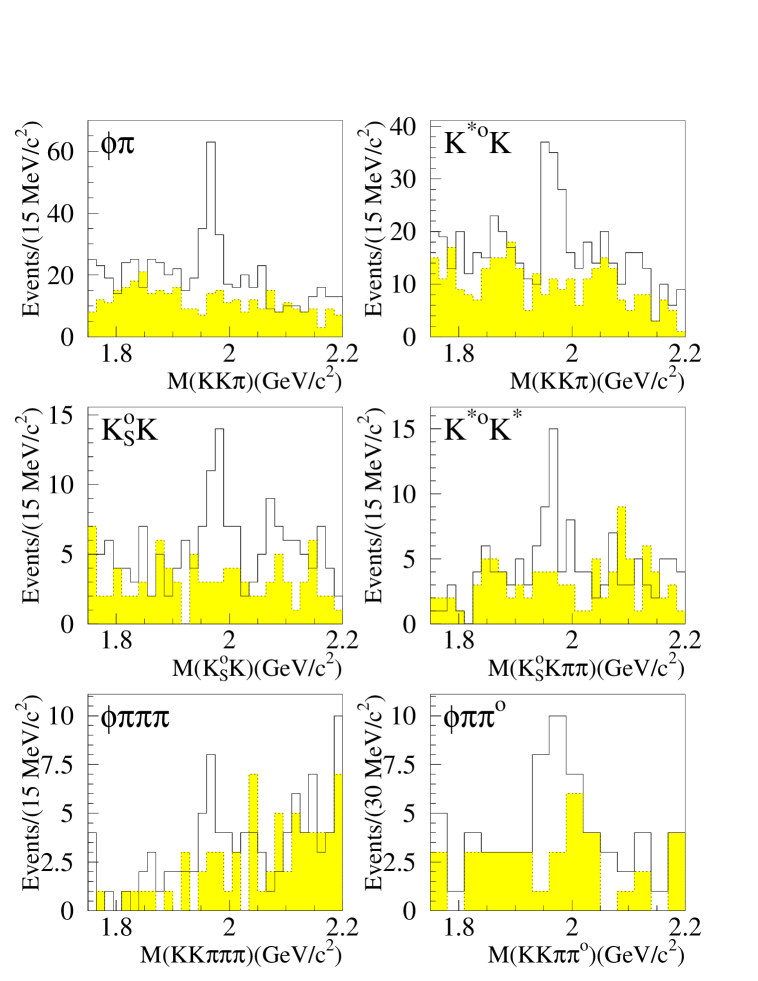
In the mass region, an excess of “right-sign”
() over “wrong-sign”
() combinations
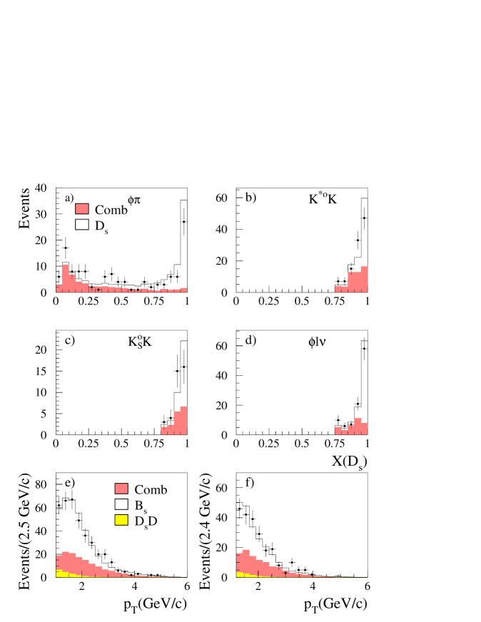
is observed in each channel (Figure 2).
The estimated number of signal events and the yields
for the combinatorial background in all the studied
modes are summarized in Table 4.
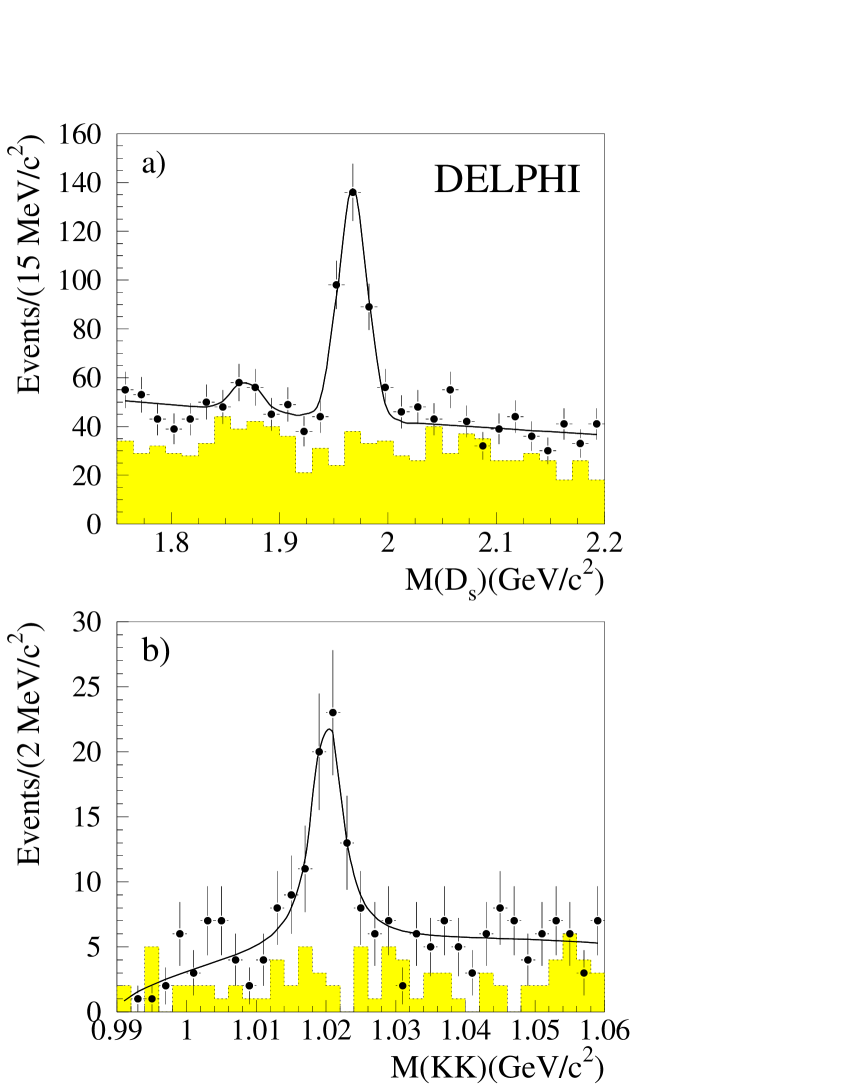
The mass distribution for non-leptonic decays has been
fitted with two Gaussian distributions of equal widths to account for the
and signals and a polynomial function for the combinatorial
background. The mass has been fixed at the nominal value of
[19].
The overall mass distribution for non-leptonic decays is shown in
(Figure 3a). The fit yields a signal of
decays in “right-sign” combinations, centred at a mass
of with a width of .
decay modes
Estimated signal
Combinatorial background / Total
Table 4: Numbers of signal events and fractions of
combinatorial background events measured in the different
decay channels. The level of the combinatorial background has
been evaluated inside
a mass interval of () centred on the measured
() mass.
3.3.2 Semileptonic modes
Selected events show an excess of “right-sign” with respect
to “wrong-sign” combinations (Figure 3b).
The invariant mass distribution for “right sign” events
has been fitted with a Breit–Wigner distribution to account for the signal
and a
polynomial function to describe the combinatorial background.
The fit gives events (see Table 4) centred at a
mass of with a total width () of
.
3.4 Selection of the inclusive channel
Inclusive semileptonic decays are reconstructed by
requiring, in the same hemisphere, a high lepton and a reconstructed
.
This analysis is expected to be more efficient than analyses based on
completely reconstructed , at the cost of a higher
background. The extra contamination comes mainly from combinatorial
pairs and from non-strange -decays. In order to avoid a statistical overlap with the sample
considered previously, all triplets
selected in the channels containing
a in the final state have been excluded from the
present sample. The analysis of the channel has been performed using
94-95 data only. Leptons are required to have a momentum
and a transverse momentum larger than and
respectively. A pair of oppositely
charged identified kaons is considered as a candidate provided
their combined momentum is above . Considering the
remaining particles of charge opposite to the lepton, the hadron with the
highest momentum projected along the direction is associated to
the decay vertex. The
vertex is fitted, and the pseudo-track is
reconstructed and fitted with the lepton track to estimate
the decay vertex.
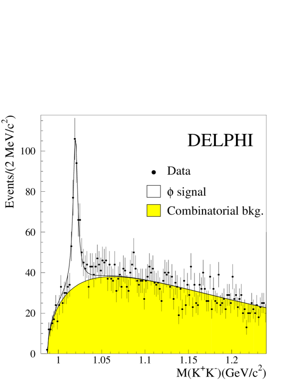
The mass distribution of the pairs has been
fitted with a Breit-Wigner function to account for true mesons
and a polynomial function for the combinatorial background (Figure 4). Accepting events within of the fitted mass,
where corresponds to the fitted width of the signal, 441
events are retained, including a combinatorial background of
.
3.5 Sample composition
The lifetime and the oscillations of mesons have been studied
selecting, in the sample, right-sign events lying in a mass
interval of () centered on the measured
() mass and, in the sample, events with the
candidate meson in a mass interval of centered
on the measured mass.
The following components, entering into the selected sample, have
to be considered:
•
: fraction of candidates from the combinatorial background:
it has been evaluated from the fit of the mass distributions on
and events;
•
: fraction of candidates coming from events
having a fake lepton and a real or meson
(in the analysis this category includes also events
containing true leptons and mesons coming from charm decays or
light quark hadronization);
•
: fraction of candidates
in which the high lepton originates from a “cascade” decay
();
•
: fraction of semileptonic decays
of non-strange mesons
•
: fraction of semileptonic decays
of the meson.
Only the last four components (i.e. background and signal coming
from physical processes) will be detailed in the following: the
estimation of the combinatorial background has been already reported
in previous sections.
3.5.1 Composition of the sample
In the sample the signal of the “right” sign correlation
is dominated by semileptonic decays; other minor sources of candidates are:
•
: a possible contribution from this source (-fake )
would give the same contribution in right and wrong sign candidates.
Since no excess has been observed in wrong sign candidates this component
has been neglected.
•
: it is the expected fraction of “cascade” decays
()
followed by the semileptonic decay
yielding right-sign pairs
(referred also as ).
This background corresponds approximately to the same number
of events as the signal [20], but the selection
efficiency is lower because of the requirement of a high lepton and of
a high mass of the system.
These selection criteria reduce the background
fractions to the values reported in Table 5.
Others
Table 5: Ratio between and signal yields
in the three classes.
Quoted errors on these fractions result from the uncertainties
on the branching
fractions of the contributing processes and from the errors
on the respective experimental selection efficiencies.
•
: two contributions to this fraction have been considered:
–
: the fraction of events from
and
decays
in which a has been misidentified as a
which give candidates in the mass region.
If the is accompanied by an oppositely charged lepton
in the decay , it looks like a
semileptonic decay.
The fractions
and
have been estimated for
the and
decay channels, respectively.
–
A pair from a non-strange B meson decay,
with the lepton
emitted from a direct B semileptonic decay, may come from the decay
.
The production of in B decays not originating from , has been measured by CLEO
[21], but no measurement of this production in
semileptonic decays exists yet. This process implies the production
of a followed by its decay into
. This decay is suppressed by phase space
(the system has a large mass) and by the
required additional pair. A detailed
calculation shows that the contribution of this process is [22]:
Assuming a selection efficiency similar to the one for the
component the contribution of this decay channel is below 2% and,
for this reason, has been neglected in the following.
Taking into account the above components, the estimated number of semileptonic
decays in the sample of 436 candidates is . The signal composition for each decay mode is given in Table 6.
Others
-
-
-
Table 6: Estimated composition of the signal in the sample
In order to increase the effective purity of the selected sample,
signal and background fractions have been calculated on an event by event
basis using the probability density functions of and
(defined in Section 3.1):
where ,
,
,
are
the probability densities for the mesons,
the combinatorial background,
the background and
the signal events, respectively. In these expressions, is a normalisation factor such that:
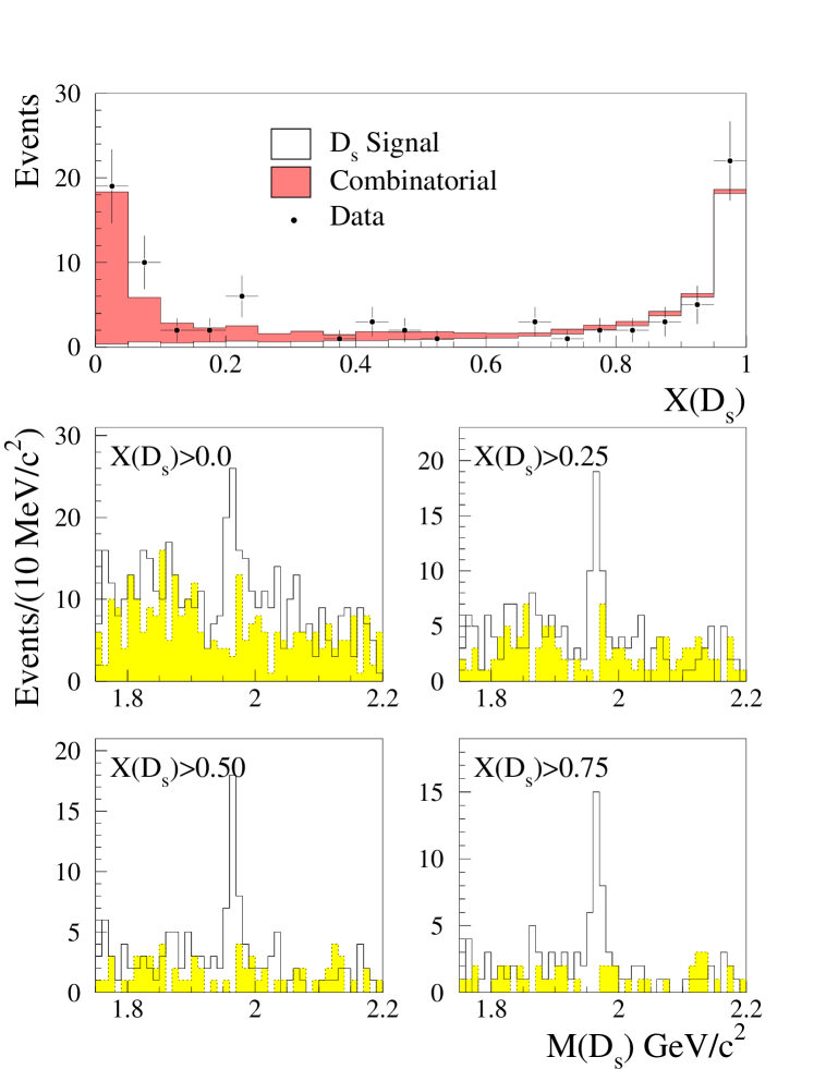
The distributions of the values of the
and variables are shown in Figure 5.
The use of this procedure is equivalent to increasing the statistics
by a factor 1.2.
3.5.2 Composition of the sample
The different contributions to candidates contained
in the selected mass interval of
around the nominal mass and corresponding to a real meson
are shown in Table 7 and have been estimated using
simulated events and measured branching fractions.
Quoted uncertainties originate from the finite Monte Carlo statistics, except for
one attached to the signal fraction which is dominated
by [23].
Source
Table 7: Estimated composition of the signal
in the sample
The number of semileptonic decays contained in this sample has
been evaluated to be .
3.6 Measurement of the B meson decay time
For each event, the decay time is obtained from the measured
decay length () and the estimate of the momentum ().
The momentum is estimated using the measured energies:
The neutrino energy is obtained from the measured value of
(see Section 3.1). The agreement between data and simulation on has
been verified using the side bands of the sample.
In order to have enough statistics to perform this test,
cuts not correlated with the missing energy have been relaxed.
In addition, to verify the resolution on the energy estimate, the
studied sample has been enriched in light quark events by applying an
anti–b-tagging cut (Section 2.4).
A relative shift of has been measured and the
simulation has been
corrected. Figure 6 shows the agreement
between data and simulation after having applied this correction. The neutrino resolution has been improved by correcting
by a function of
energy222here means “observed decay products of
”, including also the decays where the is not fully
reconstructed: specifically
and
and which has been determined from simulated signal events:
The data-simulation
agreement on has been verified on the selected signal events after
subtraction of the combinatorial background (estimated from
events selected in side-bands
of and signals)
(Figure 6).
3.7 Proper time resolution and acceptance
The predicted decay
time distributions have been obtained by convoluting the theoretical
distributions with resolution functions evaluated from simulated events.
Due to different resolutions on the decay length, different parametrizations of
the proper time resolution have been used for
three different classes in the sample: decays,
other non-leptonic decays and semileptonic decays.
Different parametrizations have been also used for the two Vertex
Detector configurations installed in 91-93 and in 94-95.
The proper time resolution is obtained from the distribution of the difference
between the generated () and the reconstructed () time.
The following distributions have been considered:
•
is the resolution function for direct
semileptonic decays. is parametrized, for the sample, as the sum of three
Gaussian distributions. The width of the third Gaussian is taken
to be proportional to the width of the second Gaussian.
In the analysis a fourth Gaussian distribution has been added. The parameters related to the decay length and proper time resolutions,
and respectively,
and the relative fractions are listed in Table 8.
A typical parametrization of the resolution, for the sample,
is shown in Figure 7 for the decay mode obtained with the 94-95
Vertex-Detector configuration.
•
is the resolution function applied to
“cascade“ events. Since the charm decay products have been only partially reconstructed in
these events, the momentum of the candidate is underestimated
giving a long positive tail in the proper time resolution
function. The function,
, is well described by a Gaussian
distribution convoluted with an exponential distribution. The variation of
the shape of this distribution with the
generated proper time has been neglected.
sample
decay mode
(92-93)
0.16
0.08
1.04
0.16
-
0.50
0
(94-95)
0.16
0.08
0.98
0.16
-
0.28
0
other non-leptonic (92-93)
0.11
0.07
0.39
0.16
5
0.26
0.07
other non-leptonic (94-95)
0.11
0.07
0.37
0.16
3
0.16
0.02
(92-93)
0.14
0.075
0.31
0.15
6
0.29
0.09
(94-95)
0.14
0.075
0.31
0.15
6
0.21
0.07
sample
0.13
0.08
0.28
0.09
0.32
0.19
1.06
0.42
0.31
0.41
0.10
Table 8: Fitted values of the parameters of the resolution function
obtained, on simulated events, for the and samples.
Distortions on the reconstructed proper time can be due to a non-uniform
reconstruction efficiency as a function of the true proper time (acceptance). Non-uniform efficiencies have been observed, on simulated events,
in the decay modes , and
because of the selection criteria on . This effect has been taken into account by inserting in the fitting function,
for those channels, an acceptance function ()
parametrized on simulated events.
4 Measurement of the lifetime
The meson lifetime has been studied using the signal
sample (Section 3.5) and a background sample
containing events selected in the sidebands of () candidates.
Sidebands events are “right” sign events lying in the mass interval
for the hadronic decays and
“right” sign events lying in the mass interval
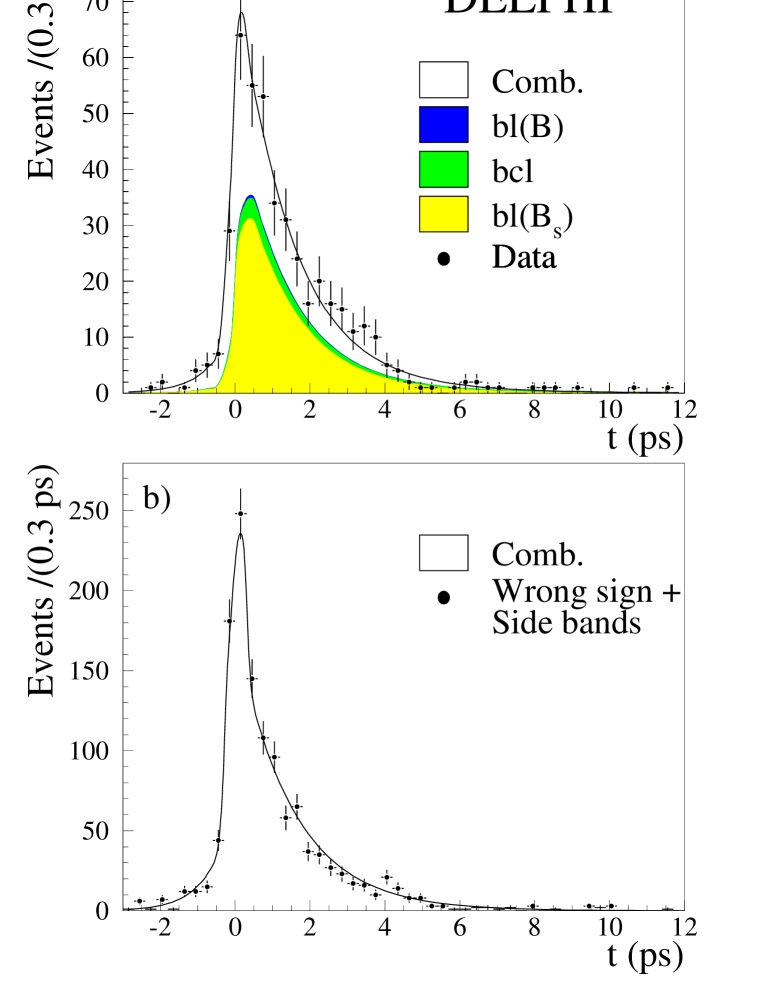
for the semileptonic decays. In the analysis “wrong” sign candidates have been also included
in the background sample.
This background sample is assumed to have the same proper
time distribution as the combinatorial background in the signal
sample. This assumption has been verified using the simulation.
The probability density function used for events in the signal region
is given by:
where and are the measured and true
proper times respectively. The different probability densities are expressed as convolutions of the
physical probability densities with the appropriate resolution () and acceptance ()
functions:
•
for the signal:
•
for the background coming from non strange mesons:
where runs over the various B-hadrons species contributing to this
background,
•
for the “cascade” background:
•
for “fake lepton” candidates the function
has been parametrized using simulated events;
•
for the combinatorial background two different parametrizations
have been used:
–
sample.
Three distributions have been used for each of the three classes of decay time
resolution (see Section 3.7).
A negative exponential for poorly measured
events (with negative lifetime ),
an exponential distribution for the flying background
(with lifetime ) and a central Gaussian for the non-flying one.
The seven parameters (, , , and )
have been fitted independently for the 92-93 and 94-95 data samples.
The parameter are taken to be different for the three classes
of decay time resolution.
–
sample. The combinatorial background shape has been described with a sum
of four smeared exponentials ().
lifetime fit has been performed simultaneously on the signal and
background samples.
All parameters describing the shape of the background time distributions
in the and samples are left as free parameters.
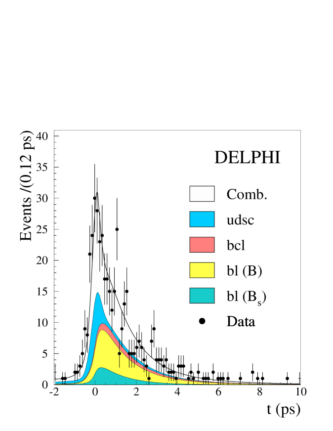
Results of the fit are shown
in Figure 8 ( sample) and
in Figure 9 ( sample).
Table 9 summarizes the different lifetimes measurements with their
statistical errors.
Decay mode
Data set
(92-95)
(92-95)
(92-95)
(94-95)
(94-95)
(94-95)
(92-95)
(94-95)
Table 9: lifetime determinations using the and events samples.
4.1 Systematic errors on the lifetime
Systematic uncertainties attached to the lifetime determination
are summarized in Table 10.
Systematics
variation in
discrim. var.
discrim. var.
resolution
acceptance
Simulated evts. statistics
Total Syst.
Table 10: Different contributions to the systematic uncertainty attached
to the lifetime measurement.
The main contributions to the systematic uncertainties come from:
•
Systematics from the evaluation of the purity.
–
sample: The different fractions for signal and background events have been calculated
on an event by event basis. The expressions
defining the effective purities are given in Section 3.5.1. The value of
has been varied according to the statistical
uncertainties of the fitted combinatorial background fractions present in
the different, or , mass
distributions. The value of has been varied
according to the errors given in Table 7 and in Table 6,
which takes into account both the statistical error from the simulation and the
errors on measured branching ratios. The evaluation of the systematics due to the procedure used to evaluate
the purity on a event by event basis has been evaluated in two steps.
The distributions of the variable (Figure 5)
for signal and background events have been re-weighted with as linear
function in order to maximize the Data-simulation agreement:
The linear behaviour of the correction has been chosen because of the limited
statistics in the data: it has been verified that a quadratic correction
does not change the result significantly. The fit has been redone with this new probability distribution and the
variation of the fitted lifetime value (+0.008 )
has been taken as the systematic error. Because of the agreement between data and simulation
(Figure 5-e and 5-f)
for the distribution, the systematic error associated to this variable
has been evaluated varying its distributions by the uncertainties of the
parametrization obtained from simulated events.
–
sample: In this analysis the fractions of signal and background events have not been calculated
on an event by event basis. The systematic uncertainty due to the variation
of the fractions have been obtained by varying
these parameters by the errors reported in Table 7
and in Table 4.
The systematic uncertainty attached to the fraction, affecting only
the sample, has a negligible effect on the global result.
•
Validation of the fitting procedure
using simulated events. The fitting method has been verified on pure simulated events:
the measured value on this sample has been
in agreement with the generated value
(). The statistical error of this verification
has been included in the systematic uncertainties. A similar check has been performed on the sample giving
.
Since the statistical weight of the channel is small
compared to the full sample, the error on the fitting procedure is
dominated by the statistics of simulated events.
•
Systematic from the proper time resolution. Uncertainties on the determination of the resolution on the proper time receive
two contributions: one from errors on the decay distance evaluation and the other
from errors on the measurement of the momentum.
The agreement between real and simulated events on the evaluation of the
errors on the decay distance has been verified by comparing the widths of
the negative part of the flight distance distributions, for events which are
depleted in B-hadrons. The difference between the two widths has been found
to be of the order of 10%. The systematic on momentum has been evaluated by comparing
the momentum distribution on simulated events with the distribution,
background subtracted, obtained from the data sample (see Section 3.5.1).
Effects from shift and width differences between the two distributions
have been considered by changing the shape of the distribution of simulated events;
it has been found that the main systematics comes from difference in width:
the width on data has been estimated to be larger by a factor . Taking into account these two effects the uncertainty on the time resolution
has been, conservatively, evaluated by varying the parameters and
of the resolution functions (see Table 8)
by 10. Uncertainties on the acceptance determination have been also considered:
the parameters entering in the definition of the acceptance function have
been varied according to the errors given by the fit on simulated events.
The final result is:
(15)
5 Lifetime difference between mass eigenstates
The (or ) mesons are superpositions of the two mass eigenstates:
The probability density for N semileptonic decays
is proportional to:
(16)
where =
. The semileptonic partial widths for and are assumed to be
equal since only CP-eigenstates could generate a difference
(semileptonic decays are not CP-eigenstates). It follows that the two exponentials are multiplied by the same factor and
the probability density for the decay of a or at time is
given, after normalization, by:
(17)
where
,
.
Two independent variables are then considered: 333
does not coincide with the measured lifetime if
is different from zero
and . As the statistics in the sample is not sufficient to fit
simultaneously and ,
the method used to evaluate consists in calculating
the log-likelihood
for the time distribution measured with the and samples
and deriving the probability density function for by
constraining to be equal to
[19]444
It has been assumed that .
( is predicted in [1]).
The log-likelihoods function described in Section 4
have been modified by replacing the physical function
()) by Equation (17) and
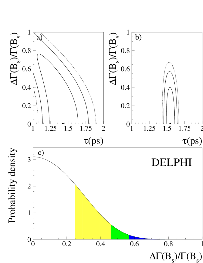
they have been added. The log-likelihood sum has been minimized in the plane
and the difference with respect to its minimum ()
has been calculated (Figure 10-a):
The probability density function for the variables and is then proportional to:
The probability distribution is obtained by convoluting
with the probability density function
, expressing
the constraint , and normalizing the result:
where
The upper limit on , calculated from , is:
This limit takes into account both statistical uncertainties and the systematic
coming from the uncertainty on the lifetime. The systematic uncertainty originating from other sources has been evaluated
by convoluting
with the probability density functions of the corresponding parameters:
where are the parameters considered in the systematic uncertainty and
are the corresponding probability densities. Since the method implies heavy numerical integrations over a -dimensional grid
only two systematics have been considered here: the purity in
meson of the selected sample and the acceptance.
This approximation is justified since
systematic uncertainties are expected to be small
(as they are in the lifetime measurement) and dominated by these two parameters. The probability distribution, obtained with the inclusion of the systematics,
is shown in Figure 10-c,
the most probable value for is and the upper limit at 95% confidence
level is:
It should be noted that the world average of the lifetime
cannot be used as constraint in such analysis,
since it depends on and on
. Moreover, this dependence is also different for
different decay channels.
In the case the expression of the average lifetime
is given by:
(18)
6 Study of - oscillations
The study of - oscillations requires the tagging of the sign
of the quark in the meson at the decay and production
times. The algorithm used for the tagging at production time
has been tuned in order to have the best performances on the sample,
where all the charged particles from the
decays have been reconstructed.
6.1 tagging at production time
The signature of the initial production of a quark
in the jet containing the or
candidate is determined using a combination of different variables which are
sensitive to the initial quark state following the same technique as
in Section 3.1. For each individual
variable , the probability density functions
for () quarks are
obtained from the simulation
and the ratio is computed. The combined
tagging variable is defined as:
(19)
The variable varies between -1 and 1. High values of
correspond to a high probability that a given
hemisphere contains a quark in the initial state. If some of the
variables are not defined in a given event, the corresponding
ratios are set to 1, corresponding to equal probabilities for the initial
state to be or . An event is split into two hemispheres by the plane passing
through the beam interaction point and perpendicular to the direction
of the candidate;
then nine
discriminant variables have been selected for this
analysis.
Five variables are defined in the hemisphere opposite
to the meson,
in which reconstructed charged particles have been used:
•
the mean hemisphere charge which is defined as :
(20)
In this expression n is total number of charged particles in the hemisphere,
and are, respectively,
the charge and the momentum of
particle is the unit vector along the thrust
axis and =0.6;
•
the weighted sum of the charges of particles with tracks identified as kaon candidates:
;
•
the sum of the charges of tracks having significant impact parameters
with respect to the event primary vertex;
•
the sum of the charges of the particles whose tracks are
compatible with the event primary vertex;
•
the momentum transverse to the jet axis multiplied by the charge of the identified lepton
candidate with the highest momentum.
These variables have been combined to form the discriminant variable
.
Another set of three variables are evaluated in the hemisphere
which contains the meson candidate and
only tracks not included in the candidate decay products
have been used in their determination
555 In the analysis all the decay products are
identified and removed, for more inclusive analyses this is only partially possible.
They are:
•
the mean hemisphere charge, computed using (20) with
directed along the reconstructed momentum of
the candidate;
•
the rapidity with respect to the direction of the thrust axis multiplied by the
charge of the identified kaon candidate
with the highest momentum having a trajectory compatible with the primary
vertex
(this algorithm aims at reconstructing the fragmentation kaon produced with
the , this kaon has a sign opposite to the quark contained in
the meson);
•
the momentum of any reconstructed candidate multiplied by the
charge
of the proton from its decay (same principle as in the previous item when
a baryon instead of meson is produced).
These variables have been combined to form the discriminant variable
.
In addition the distribution of the polar angle of the direction of the thrust
axis, common to both hemispheres, is also used to benefit from the forward-backward
asymmetry of the quark production relative to the electron beam axis.
6.2 Measurement of the tagging purity in events with an exclusively
reconstructed
The high statistics sample of exclusively reconstructed ,
accumulated in 1994-95, has been used to check the tagging procedure.
The purity of the tagging at production time, , has been measured
on those events using the analysis of the mixing.
The candidates have been selected by reconstructing the decay chain
followed by or
.
The selection criteria rely mainly on the small mass difference between
and mesons [24].
The measurement of the mixing is performed by correlating
a) the sign of the charge, which
tags the B flavour at decay time (since in these events are mainly
produced from and
from ), with b) the global tagging variable,
,
evaluated in the hemisphere opposite to the and
obtained by combining the five first quantities defined in the
previous section.
If the meson, decaying into a , has oscillated,
the
charge and the value of the variable are expected to
be of unlike sign.
The mass difference, , between the two physical states
of the system
is obtained from the study of the decay distance distribution for unlike
and like sign events. Details of the analysis can be found in
[24].
The amplitude of the time dependent oscillation is sensitive to the
probability of correctly tagging events as unmixed and mixed candidates.
A fit has been performed, fixing the mass difference to the world
average [23], and leaving as a free parameter.
The fit has been repeated for different minimum values of the global
tagging variable . Results are reported in Table 11,
together with the predictions from the simulation. The fraction
of events remaining after the cut on the tagging variable
is also reported.
Data
Simulation
1.0
1.0
0.88
0.89
0.77
0.78
Table 11: Values of obtained from the
analysis of exclusively reconstructed for different cuts on
the value of
the tagging variable . Also reported is the fraction of events
remaining after the cut. Expectations from the simulation are also given.
The tagging efficiency, estimated using the sample,
is consistent within
its uncertainty with the expectation from the simulation.
The selected sample of exclusively reconstructed still contains a
significant fraction of events originating from charm and light quarks.
In order to study the distribution of the tagging variable , the
b-tag probability for all tracks in the event has been required to be smaller
than [16].
The fraction of non-b events in the remaining
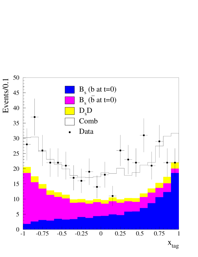
sample is estimated to be . The distribution of the product between
the charge and the value of the tagging variable
is shown in Figure 11–a, together with the expectation
from the simulation.
Another check has been performed by selecting events with an exclusively
reconstructed accompanied by a lepton of opposite
charge. This sample is highly enriched in , but has a limited
statistics. However, it allows the study of the tagging
variable defined, in the same hemisphere as the -lepton
candidate, by combining the other three variables mentioned
in the previous section.
The variable which quantifies the presence of an identified kaon
of highest momentum compatible with the primary vertex has been removed from
the definition of .
The distribution of the product between the charge
and the value of the tagging variable, , is shown in
Figure 11–b together with the expectation from
the simulation.
The selected sample do not have enough statistics to perform
a quantitative check. The distributions
expected from the simulation and measured data, using the
sample, are found to be compatible within statistics (Figure 12).
6.3 Tagging procedure
An event is classified as a mixed or an unmixed candidate according to
the relative signs of the electric charge, ,
and of the variable.
Mixed candidates have , and unmixed
ones . The probability, , of tagging the or the
quark correctly from the measurement of has been
evaluated using a dedicated simulated event sample and has been found
to be, in the sample, % in 94-95 data and
% in 92-93 data. In the sample the tracks
from the decay have not been all reconstructed.
The tagging purity is lower with respect to the one estimated in the sample
due to some possible misidentification between primary and secondary tracks
present in the same hemisphere as the meson. The value found in simulated events is
().
To improve the tagging purity further, the shape of the
distribution can be included in the analysis. Four purities enter in the analysis:
-
: tagging purity for the direct decays;
-
: tagging purity for “cascade” decays;
-
probability of
classifying background candidates as mixed or as unmixed
(computed on sidebands events);
-
probability of
classifying fake lepton candidates as mixed or as unmixed.
using as a discriminant variable each of these purities
is replaced by the function ,
where is the probability density function. The global probability density function has been divided by the sum
( and ) in order
to keep, for the signal part, the relation . The functions entering in the final likelihood are then re-defined as:
The effective tagging purities obtained, in the sample, with this method correspond to %
for 94-95 data and to % for 92-93 data.
6.4 Fitting procedure
From the expected proper time distributions and the tagging probabilities,
the probability functions for mixed and unmixed events candidates have been
computed
666In the following, only the probability function for mixed events
is written explicitly; the corresponding probability for unmixed events can be
obtained by changing .:
(22)
where is the reconstructed proper time.
The analytical probability densities are as follows, with being the true
proper time:
•
mixing probability.
(24)
•
“cascade” background mixing probability.
(30)
Note that the two terms contributing to the are due to the
fact that, in the decay
, the lepton can originate from either
mesons. The contribution can then be simplified in the
expression and becomes, mixing independent:
•
non-strange -hadrons mixing probability.
(34)
•
mixing probability for candidates from light quark events or fake leptons:
(35)
•
combinatorial background mixing probability:
(36)
The parameters entering in the proper time distribution for this
background have been determined in the lifetime fit.
The oscillation analysis has been performed in the framework of the amplitude
method [25] which consists in measuring, for each value of
the frequency , an amplitude and its error
. The parameter is introduced in the time evolution of pure
or states so that the value corresponds to
a genuine signal for oscillation:
The 95 C.L. excluded region for is obtained by evaluating the
probability that, in at
most 5 of the cases, a real signal having an amplitude equal to unity
would give an observed amplitude smaller than the one measured.
This corresponds to the condition:
In the amplitude approach it is possible to define the exclusion
probability, that is the probability that a certain value
lies in an excluded region if the generated was very
large ().
The sensitivity is the value of corresponding to 50 % of
exclusion probability.
Using the amplitude approach (Figure 13), and
considering only statistical uncertainties,
a limit has been obtained:
(38)
with a corresponding sensitivity at .
At = 10 , the error on the amplitude is 0.85.
Several checks have been done to verify the reliability of the amplitude fit:
the proper time distributions for mixed and unmixed events have been verified
to be well reproduced by the fit (Figure 14-a,-b) and the ratio between
mixed events and the total number of events in bins of the proper time
has been compared with the expected distribution for
and . These values have been chosen to illustrate
the behaviour of the expected oscillation curve for () and
() (Figure 14-e).
It could be seen that the oscillation curve at
(where is close to 1) fits the data better than the corresponding curve
at (where is compatible with 0), as expected from the definition of .
6.5 Study of systematic uncertainties
Systematic uncertainties have been evaluated by varying the parameters which
have been kept constant in the fit, according to their measured or
expected errors, using the
formula [25]:
and
indicate the variations of the amplitude, in the central value and
in the error, due to the considered systematics. Three main sources of systematic uncertainties have been identified:
•
Systematics from the tagging purity.
–
sample. The studies done in Section 6.2 show that, using the tagging variables
in the opposite hemisphere and
requiring
, the difference between the values of the tagging
purity measured in real and simulated events is
= -0.01 0.02. It has been verified
that the real and the simulated distributions for the
tagging purities agree in both hemispheres. The systematics coming from the control of the tagging purity has been
evaluated by varying the probability distributions of the discriminant
variable for and quarks in a way to induce
an absolute variation on the effective value of the tagging purity of .
–
sample.
The agreement between data and simulation has not been checked for this sample;
a conservative absolute variation of 5% in the tagging purity has been assumed.
•
Systematics from the purity. The same procedure already applied for the lifetime measurement has been used.
•
Systematics from the resolution on the B decay proper time. The same procedure already applied for the lifetime measurement has been used.
In addition, the systematic error due to the variation of the proper
time distribution of the combinatorial background,
has been considered: the parameters used to define the
background shape,
in the lifetime fit, have been varied according to their fitted errors.
The inclusion of systematic uncertainties lowers the sensitivity
to without affecting the C.L limit. In Table 12
the amplitude values are reported, together with their statistical and systematical errors,
for five different values of .
-0.638
0.304
0.112
0.033
0.037
0.400
0.118
0.060
0.182
0.561
0.069
0.098
1.343
0.846
0.160
0.180
0.867
1.241
0.285
0.389
Table 12: Amplitude values with statistical and systematic errors
for three different values of
The exclusion probability of is 54% while
the probability of obtaining a limit on higher than the actual one is
38% (Figure 15-c). Figure 15-a and Figure 15-b
represent, respectively, the error on the amplitude and the exclusion probability
as a function of .
7 Conclusion
A sample of 436 candidate events has been
selected from about 3.6 million hadronic decays accumulated by
DELPHI between 1992 and 1995, using seven different decay modes.
The number of events coming from semileptonic decays has been estimated
to be in this sample. In addition, a sample of 441 ,
containing semileptonic decays, has been also used.
Events contained in the sample, with a reconstructed and
have been removed from this last sample. Using these samples, three analyses have been performed.
The lifetime has been measured and a limit on the fractional width
difference between the two physical states has been set:
This last result has been obtained under the hypothesis that
. The study of oscillations sets a limit at 95% C.L. on the mass
difference between the physical states:
(40)
with a corresponding sensitivity equal to . Previous DELPHI results obtained with and samples
([26],[20]) are superseded by the analyses
presented in this paper.
Acknowledgements
We are greatly indebted to our technical
collaborators, to the members of the CERN-SL Division for the excellent
performance of the LEP collider, and to the funding agencies for their
support in building and operating the DELPHI detector. We acknowledge in particular the support of Austrian Federal Ministry of Science and Traffics, GZ 616.364/2-III/2a/98, FNRS–FWO, Belgium, FINEP, CNPq, CAPES, FUJB and FAPERJ, Brazil, Czech Ministry of Industry and Trade, GA CR 202/96/0450 and GA AVCR A1010521, Danish Natural Research Council, Commission of the European Communities (DG XII), Direction des Sciences de la Matire, CEA, France, Bundesministerium fr Bildung, Wissenschaft, Forschung
und Technologie, Germany, General Secretariat for Research and Technology, Greece, National Science Foundation (NWO) and Foundation for Research on Matter (FOM),
The Netherlands, Norwegian Research Council, State Committee for Scientific Research, Poland, 2P03B06015, 2P03B1116 and
SPUB/P03/178/98, JNICT–Junta Nacional de Investigação Científica
e Tecnolgica, Portugal, Vedecka grantova agentura MS SR, Slovakia, Nr. 95/5195/134, Ministry of Science and Technology of the Republic of Slovenia, CICYT, Spain, AEN96–1661 and AEN96-1681, The Swedish Natural Science Research Council, Particle Physics and Astronomy Research Council, UK, Department of Energy, USA, DE–FG02–94ER40817.
References
[1] M. Beneke, G. Buchalla and I. Dunietz Phys. Rev.D54
(1996) 4419.
[2] L. Wolfenstein,
Phys. Rev. Lett.51 (1983) 1945.
[3] G. Altarelli and P.J. Franzini,
Zeit. Phys.C37 (1988) 271. P.J. Franzini, Phys Rep.173 (1989) 1.
[4] A. J. Buras, Acta. Phys. Polon.B26 (1995) 755.
[5]
A.X. El-Khadra, A. Kronfeld, P.B. Mackenzie, S.M. Ryan and J.N. Simone,
Phys. Rev.D58 (1998) 014506. C. Bernard et al. (MILC Collaboration), Phys. Rev. Lett.81 (1998) 4812. D. Becirevic, Ph. Boucaud, J.P. Leroy, V. Lubicz, G. Martinelli,
F. Mescia andF. Rapuano, Phys. Rev. D60 (1999) 074501 .
[6] P. Paganini, F. Parodi, P. Roudeau and A. Stocchi,
Physica ScriptaVol. 58 (1998) 558. F. Parodi, P. Roudeau and A. Stocchi,
Il Nuovo CimentoA112 (1999) 834.
[7] M. Beneke, G. Buchalla, C. Greub, A. Lenz and U. Nierste
Phys. Lett.B459 (1998) 631.
[8] ALEPH Collaboration, D. Buskulic et al., Phys. Lett.B377 (1996) 205.
[9] CDF Collaboration, F. Abe et al., Phys. Rev.D59 (1999) 032004.
[10] OPAL Collaboration, K. Ackerstaff et al., Phys. Lett.B426 (1998) 161.
[11] DELPHI Collaboration, P. Abreu et al.,
Nucl. Instr. and Meth. A378 (1996) 57.
[12] V. Chabaud et al., Nucl. Instr. Meth.A368
(1996) 314.
[13] DELPHI Collaboration, P. Abreu et al.,
Nucl. Phys.B418 (1994) 403.
[14] E.G. Anassontzis et al.,
Nucl. Instr. Meth.A323 (1992) 351.
[15] T. Sjöstrand, Comp. Phys. Comm.82 (1994) 74.
[16] DELPHI Collaboration,P. Abreu et al.,
Zeit. Phys.C70 (1996) 531.
[17] DELPHI Collaboration, P. Abreu et al, Zeit. Phys.C73
(1996) 11.
[18] N. Isgur, D. Scora, B. Grinstein and M. Wise,
Phys. Rev.D39 (1989) 799.
[19] Particle Data Group,
Eur. Phys. J.C3 (1998) 1.
[20] DELPHI Collaboration, P. Abreu et al., Zeit. Phys.C71 (1996) 11.
[21] CLEO Collaboration, “-Lepton Charge Correlations
in B Meson Decays: A Study of the Meson Production
Mechanism”, EPS0169 contribution to the ICHEP95, (Brussels,
July 1995).
[22] E. Golowich, A. Le Yaouanc, L. Oliver, O. Pène and
J.C. Raynal, Zeit. Phys.C48 (1990) 89.
[23] The LEP Oscillations Working Group “LEP Combined Results
on Oscillations: Results for Summer 1998 Conferences”
LEPBOSC NOTE 98/3
[24] DELPHI Collaboration, W. Adam et al.,
Zeit. Phys.C76 (1997) 579.
[25] H.G. Moser and A. Roussarie, Nucl. Instr. and
Meth.A384 (1997) 491.
[26] DELPHI Collaboration, W. Adam et al.,
Phys. Lett.B414 (1997) 382.
Figure 1: The plot on the top shows the distribution of the
discriminant variable for the channel in 94-95 data.
The points with error bars represent the data, the white
histogram shows the contribution from the simulated signal and the shaded
histogram shows the contribution
coming from simulated background events.
It could be seen that the is able to discriminate the
signal () from the combinatorial background.
The four figures on the bottom show the effect, on the
signal in the 94-95 data, of a cut on the discriminant variable
(white histograms represent “right-sign” events while shaded histogram
show “wrong-sign” events). Figure 2: Invariant mass distributions for candidates in
six non-leptonic decay modes
(, , , ,
and ).
The last three decay modes have been reconstructed using only the
94-95 statistics. The corresponding distribution for wrong-sign
combinations are given by the shaded histogramsFigure 3: a) Invariant mass distributions
for candidates in non-leptonic decay modes
(, , , , and
).
b) invariant mass
distribution for candidates selected in the two semileptonic decay
modes. The corresponding distribution for wrong-sign combinations are
given by the shaded histograms. The curves show the result of fits
described in the text.Figure 4: invariant mass distribution of the candidates.
The curves show the result of the fit described in the text
(the signal and the combinatorial background components are represented
by the white and shaded histograms respectively).Figure 5: The plots illustrate
the agreement between data and simulation
for the variables used in the estimate of the purity
on an event by event basis.
a),b),c) and d) show the distributions for the channels
, , and
respectively. White histograms and shaded histograms represent the
signal and the background respectively.
e) and f) show the distributions for the samples
selected with ( and )
and (all the others) respectively.
For the distribution the and the combinatorial background
are considered separately.Figure 6: The plot on the top shows the comparison between data and the simulation
for the missing energy distribution after correction (see Section 3.6).
The data (dots with error bars) and the simulation (dashed
histogram) are enriched in light quark events.
The dotted histogram shows the missing energy distribution in simulated b semileptonic
decays.
The plot on the bottom shows the comparison between the momentum distribution
for simulated events and the one estimated from data in the signal region by
subtracting the momentum distribution of events in the side
bands from that of the events in the signal region.Figure 7: The six plots on the top show the proper time resolution,
defined as the difference between the generated
time () and the reconstructed time (), in bins of generated time
on a sample of events simulated with the 94-95 Vertex Detector configuration.
The plot on the bottom shows the distribution of the
reconstructed time with the fit superimposed.Figure 8: sample.
a) Likelihood fit for events in the signal mass region.
The points show the data and the curves correspond to the different
contributions to the selected events.
b) The same as a) but for “wrong-sign” events and for events
situated in the side band region.
The labels of the signal components refers to Section 3.5.1Figure 9: sample.
Likelihood fit for events in the signal mass region.
The points show the data and the curves correspond to the different
contributions to the selected events.
The labels of the signal components refers to Section 3.5.2Figure 10: a) 68%, 95% and 99% C.L. contours of the negative log-likelihood
in the plane - evaluated on the sample.
b) Same as a) but with the constraint .
c) Probability density distribution for
;
the three shaded regions show the limits at 68 %, 95% and 99% C.L. respectively.
Figure 11: Check of the flavour tagging on the sample.
a) Distribution of the product between the global tagging variable and the
charge of the in
the hemisphere opposite to the candidate.
b) Distribution of the product between the global tagging variable
and the charge of the in the same
hemisphere as the -lepton candidate.
The full dots with the error bars represent the
data. The histogram is obtained in the simulation.
The non perfect separation is due to the mistag fraction of
but also to the - mixing.
Figure 12: The plot
shows the distribution of the discriminant variable in the sample.
The points with the error bars represent the data,
the white histogram shows the contribution from combinatorial background,
the lighter histogram the contribution from events and
the darker histograms
the contribution from the signal in which mesons produced
from or quarks have been distinguished.
The degree of separation between the and histograms quantify the tagging
purity of . Figure 13: Variation of the oscillation amplitude as a function
of .
The lower continuous line corresponds to where includes
statistical uncertainties only, while the shaded area includes the contribution from systematics. The dashed-dotted line corresponds
to the sensitivity curve. The lines at A=0 and A=1 are also given. Figure 14: Proper time distribution of mixed and unmixed events in sample (a-b) and
in the sample (c-d); the full dots with error bars represent the data, the
curves are the corresponding distributions for .
c) Ratio between the mixed events and the total number of events
in bins of proper time in the sample.
The full (dashed) line represents
the prediction for an oscillation () with .Figure 15: a) Variation of the error on the amplitude as a function of .
b) Exclusion probability vs. .
c) Lower limit probability density function vs. .