The BABAR Collaboration

July 26, 2001

We present preliminary results of a search for the decay $B^{0}\rightarrow a_{0}^{+}(980)\pi^{-}$ among 22.7 million $\mathchar 28935\relax{(4S)}\rightarrow B\kern 1.79993pt\overline{\kern-1.79993ptB}{}$ pairs collected by the BABAR detector at PEP-II. Using improved background suppression techniques and optimal signal extraction for rare decay searches, an excess of events over expected background is observed at the level of 3.7 standard deviations. This corresponds to the branching fraction ${{\cal B}}(B^{0}\rightarrow a_{0}^{+}(a_{0}^{+}\rightarrow\eta\pi^{+})\pi^{-})=(6.2_{\,-2.5}^{\,+3.0}\pm 1.1)\times 10^{-6}$, where the first error is statistical and the second is systematic. The $90\%$ confidence level upper limit is $11.5\times 10^{-6}$.

Submitted to the

$20^{th}$ International Symposium on Lepton and Photon Interactions at High Energies

7/23/2001—7/28/2001, Rome, Italy

Stanford Linear Accelerator Center, Stanford University, Stanford, CA 94309

  Work supported in part by Department of Energy contract DE-AC03-76SF00515.

1 Introduction

We present a search for the decay $B^{0}\rightarrow a_{0}^{+}(980)\pi^{-}$, where the $a_{0}$ resonance is observed in its dominant decay channel $a_{0}^{+}\rightarrow\eta\pi^{+}$. The interest in this mode stems from its potential use for measuring the CKM angle $\alpha$ [1, 2]. It was pointed out in Ref. [2] that, within the factorization assumption, the main tree contributions to the $a_{0}\pi$ decay amplitude vanish: they would imply forbidden second class currents. This simplifies the two-body analysis for the extraction of $\alpha$, and can lead to an enhanced direct $C\!P$ violation.

After a preselection, we refine the background suppression using Multivariate Analyzer (MVA) tools (Neural Net (NN) and Fisher discriminants). We use both cut-based and shape-based analyses, the latter employing a maximum likelihood technique, which together provide complementary results and cross-checks. The cut optimization procedure used in the analysis does not rely on a prior branching fraction estimate. Both inclusive and exclusive control samples are used for systematics checks, particularly with regard to the $\eta$ and $a_{0}$ resonances [3].

2 The BABAR Detector and the Dataset

The data used in this analysis were collected with the BABAR detector at the PEP-II storage ring, located at the Stanford Linear Accelerator Center (SLAC). PEP-II is an asymmetric $e^{+}e^{-}$ collider with a center-of-mass energy equal to the $\mathchar 28935\relax{(4S)}$ mass. From Nov. 1999 to Oct. 2000, a total of 22.7 million $B\kern 1.79993pt\overline{\kern-1.79993ptB}{}$ pairs has been collected by BABAR, corresponding to an integrated on-peak luminosity of approximately $20.7$$\mbox{\,fb}^{-1}$. In addition, $2.6$$\mbox{\,fb}^{-1}$ of off-peak data were taken during the same period: they have been used to validate the contribution to backgrounds resulting from $e^{+}e^{-}$  annihilation into light $q\overline{q}$ pairs.

The BABAR detector and its performance are described in Ref. [4]. The innermost component consists of a 5-layer Silicon Vertex Tracker (SVT), providing the positions of charged tracks in the neighbourhood of the beam interaction point. It is followed by a 40-layer central Drift Chamber (DCH), immersed in a $1.5$-T magnetic field, measuring the track momenta and providing a measurement of the specific ionization loss ($\mathrm{d}E/\mathrm{d}x$) for particle identification (PID). The main PID device is a unique, internally reflecting ring imaging Cherenkov detector (DIRC), covering the central region of BABAR. A Cherenkov angle $K/\pi$ separation of better than 4 standard deviations is achieved for tracks below 3${\mathrm{\,Ge\kern-1.00006ptV\!/}c}$ momentum. Photons are detected by a CsI(Tl) electromagnetic calorimeter (EMC), which provides excellent angular and energy resolution with high efficiency for energy deposits above 20$\mathrm{\,Me\kern-1.00006ptV}$. A superconducting solenoid, located around the EMC is itself surrounded by an iron flux return, instrumented with Resistive Plate Chambers to identify muons.

3 Analysis Method

3.1 Candidate Selection

A $B^{0}\rightarrow a_{0}^{+}\pi^{-}$ candidate contains a pair of oppositely-charged pions and two photons. Charged tracks are required to satisfy a set of track quality criteria, which includes cuts on their momenta (less than 10${\mathrm{\,Ge\kern-1.00006ptV\!/}c}$), transverse momenta (above 100${\mathrm{\,Me\kern-1.00006ptV\!/}c}$), and on the number of DCH hits (at least $20$). The tracks are also required to originate in the vicinity of the beam-beam interaction point. Pion candidates must fail electron selection criteria and are required to have a momentum in the center-of-mass (CM) above 2${\mathrm{\,Ge\kern-1.00006ptV\!/}c}$. A $B$ candidate is rejected if the track not used to form the $a_{0}$ has a DIRC Cherenkov angle consistent with a kaon. Photons are identified as energy deposits in the EMC, unassociated with charged tracks. They are required to have an energy above 80$\mathrm{\,Me\kern-1.00006ptV}$ in the laboratory frame (LAB), and must satisfy photon-like shower profile criteria. To be associated with an $\eta$ decay, a pair of candidate photons is required to have an invariant mass $0.470<m(\gamma\gamma)<0.615$${\mathrm{\,Ge\kern-1.00006ptV\!/}c^{2}}$, and the $\eta$ CM momentum must be larger than 0.9${\mathrm{\,Ge\kern-1.00006ptV\!/}c}$. The pion track and $\eta$ candidate form an $a_{0}$ candidate if their invariant mass falls in the range $0.9<m(\eta\pi)<1.08$${\mathrm{\,Ge\kern-1.00006ptV\!/}c^{2}}$. Reconstruction of $B^{0}$ candidates is done by vertexing all combinations of $\pi^{+}\pi^{-}\eta$ candidates in each event and applying a quality requirement on the $\pi^{+}\pi^{-}$ vertex. A $B^{0}$ candidate is characterized by two kinematic variables: the beam energy-constrained mass $m_{\rm EC}=\sqrt{E_{\rm beam}^{2}-p_{B}^{2}}$, where $E_{\rm beam}$ is half the CM energy and $p_{B}$ is obtained by applying kinematic constraints to the four-momenta of the $B$ daughters; and $|\Delta E|\equiv|E_{B}-E_{\rm beam}|$ with $E_{B}$ being the CM energy of the $B$ candidate. A candidate is retained if $m_{\rm EC}>5.21$${\mathrm{\,Ge\kern-1.00006ptV\!/}c^{2}}$ and $|\Delta E|<0.25$$\mathrm{\,Ge\kern-1.00006ptV}$.

3.2 Background Suppression

Charmless hadronic modes suffer from large amounts of background from random combinations of tracks, mostly from light quark production. In the CM frame, this background typically exhibits a two-jet structure in contrast to the spherically symmetric $\mathchar 28935\relax{(4S)}\rightarrow B\kern 1.79993pt\overline{\kern-1.79993ptB}{}$ events. Efficient background rejection is obtained by requiring the angle $\theta_{\rm T}$ between the thrust axis of the $B$ candidate and the thrust axis of the rest of the event (ROE) to satisfy $|\cos\theta_{\rm T}|<0.9$. Denoting $|\cos\theta_{\rm TP}|$ as the minimum cosine of the two angles formed by the two most energetic tracks (or neutral clusters) with respect to the thrust axis of the event, we require $|\cos\theta_{\rm TP}|<0.88$. Combinatorial background within a candidate event arises mainly from low-energy photons. Compared with decay modes containing $\pi^{0}$’s, this is a minor concern for $a_{0}\pi$ due to the higher $\eta$ mass: the fraction of events with more than one photon pair combination passing the selection cuts is at the percent level. For events with multiple candidates the one with the most energetic low-energy photon is retained.

Figure 1: Fisher (left-hand plots) and Neural Net discriminants (right-hand plots). The upper plots show the distributions for signal and background, where the signal is taken from Monte Carlo simulation and the background from on-peak sideband data. The points with error bars show the off-peak data, containing no signal. The lower plots show the signal and background efficiencies as a function of the cut applied (the small dots indicate the off-peak data).

Further discrimination is achieved by combining event shape variables using MVA techniques. A common approach uses the Fisher discriminant (denoted standard Fisher below) proposed by the CLEO Collaboration [7]. This standard Fisher is built as a linear combination of the cosine of the angle between the $B$ candidate momentum and the beam axis, the cosine of the angle between the $B$ candidate thrust axis and the beam axis, together with nine energy deposits, each defined to be the energy of charged tracks and neutral clusters of the ROE whose directions are contained in nine concentric cones centered around the $B$ direction. In our analysis, the choice of variables has been reconsidered taking into account the separation power, the correlations between the variables and the signal efficiency at fixed background rejection. For this purpose, 12 variables are selected and combined using either a linear (Fisher) or a non-linear (NN) MVA. Table 1 lists the variables which are retained together with their respective Fisher coefficients. Among thse are the six variables $L_{j}^{({\rm c})}$, $L_{j}^{({\rm n})}$ ($j=0,2,6$) defined by

$$L_{j}^{({\rm c,n})}=\sum_{i_{({\rm c,n})}}p_{i}\times|\cos\theta_{i}|^{j}~{},$$ (1)

which are the momentum-weighted sums of the cosines of the angles between the ROE charged tracks ($L_{j}^{({\rm c})}$) or neutral clusters ($L_{j}^{({\rm n})}$) and the thrust axis of the $B$ candidate. These variables provide a generalization of the discrete cones used in the standard Fisher discriminant.

Figure 2: Comparison of the background versus signal efficiencies for NN (solid line), the Fisher (dashed line), and the standard Fisher (dashed-dotted line) discriminants.

Figure 1 shows the distributions of the Fisher and NN discriminants for signal and background, the former taken from Monte Carlo simulation and the latter from on-peak sideband data (histograms) and from off-peak data (points with error bars). The lower plots show the resulting signal and background efficiencies as a function of a cut applied on the output values of the discriminants. Figure 2 depicts the background versus signal efficiencies for the standard Fisher discriminant and the 12-variable MVAs adopted in this analysis. A 17% relative increase of the signal efficiency is obtained for NN with respect to the standard Fisher at the benchmark of 5% background retention. Table 2 summarizes the performances of the three MVA discriminants. The NN, being the discriminant which provides the best signal efficiency, is used for the signal extraction in this analysis, while keeping the Fisher for cross-checks.

Table 1: The 12 event-shape variables used as MVA inputs with their corresponding Fisher coefficients.

Variable name	Description	Fisher coefficient
$R_{2}$	Second Fox-Wolfram moment	$0.40$
$|\cos\theta_{\rm T}|$	Angle: $B$/ROE thrust axis	$-0.71$
$|\cos\theta_{\rm S}|$	Angle: $B$/ROE sphericity axis	$-0.89$
$|\cos(B,z)|$	Angle: $B$ direction/beam axis	$-0.88$
$|\cos(B({\rm T}),z)|$	Angle: $B$ thrust/beam axis	$-0.79$
$|\cos\theta_{\rm TP}|$	Minimum cosine of ROE tracks/clusters	$0.54$
$L^{\rm n}_{0}$	Neutral zeroth-order angular function	$0.35$
$L^{\rm n}_{2}$	Neutral second-order angular function	$-1.02$
$L^{\rm n}_{6}$	Neutral sixth-order angular function	$-0.69$
$L^{\rm c}_{0}$	Charged zeroth-order angular function	$0.38$
$L^{\rm c}_{2}$	Charged second-order angular function	$-0.51$
$L^{\rm c}_{6}$	Charged sixth order angular function	$-0.66$
Offset	Centers the sum of signal and background at zero	$1.49$

Table 2: Results on the separation and the signal efficiency at the benchmark of 5% background retention for the standard Fisher discriminant and the two MVAs used in this analysis.

Type	$\langle s^{2}\rangle$	$\epsilon(S)({\rm at}~{}\epsilon(B)=5\%)$
Fisher (standard)	$0.44$	$0.52$
Fisher (12-var.)	$0.48$	$0.57$
Neural Net (12-var.)	$0.50$	$0.61$

3.3 Cut-Based Analysis

The signal extraction is based on counting data events found in a signal region (SR) and subtracting from this the expected background yield. To find an optimal set of signal selection criteria, balancing between background rejection and signal efficiency, we use the procedure described in the appendix. The criterion it applies is to minimize the expected confidence level for the null hypothesis “there is no signal in the data sample”. Cut optimization is performed on the MVA output only, resulting in the requirements $x_{\rm opt}^{\rm out}({\rm NN})>0.6$ and $x_{\rm opt}^{\rm out}({\rm Fisher})>0.7$, respectively.

Table 3: Selection efficiencies, expected signal and background yields for the cut-based analysis using Fisher or NN. When two errors are given, the first is statistical and the second is systematic. We quote upper limits as the main results and compute branching fractions and statistical significances, should the observed excess be interpreted as evidence for a signal. The systematic errors are discussed in Sec. 4.

	Fisher	Neural Net
Signal efficiency ($\%$)	$14.2$	$14.6$
Events in signal box	20	18
Events in GSB	242	197
Expected background
events in signal box	$9.6\pm 0.6\pm 1.4$	$7.9\pm 0.6\pm 1.1$
Branching fraction $(\times 10^{-6})$	$8.2_{\,-3.0}^{\,+4.6}\pm 1.4$	$7.8_{\,-2.7}^{\,+4.0}\pm 1.2$
Statistical significance	$3.0\sigma$	$3.1\sigma$
$90\%$ CL Upper limit $(\times 10^{-6})$	$15.3$	$14.5$

The SR is defined as $|m_{\rm EC}-5.28|<0.006$${\mathrm{\,Ge\kern-1.00006ptV\!/}c^{2}}$, $|\Delta E|<0.070$$\mathrm{\,Ge\kern-1.00006ptV}$ and $0.517<m(\gamma\gamma)<0.587$${\mathrm{\,Ge\kern-1.00006ptV\!/}c^{2}}$. The background contamination in the SR is estimated from the two-dimensional Grand Sideband (GSB): $|\Delta E|<0.25$$\mathrm{\,Ge\kern-1.00006ptV}$ and $5.210<m_{\rm EC}<5.263$${\mathrm{\,Ge\kern-1.00006ptV\!/}c^{2}}$, assuming for the corresponding background shapes a second-order polynomial for $\Delta E$, and an ARGUS function [8] for $m_{\rm EC}$. The signal efficiencies ($\epsilon$), event yields (${\cal N}$) and the expected backgrounds ($N_{b}$) are given in Table 3 for Fisher and NN. The corresponding branching fractions are obtained from the expression

$${{\cal B}}=\frac{{\cal N}-N_{b}}{\epsilon\,N_{B\bar{B}}}~{},$$ (2)

where $N_{B\bar{B}}=(22.74\pm 0.36)\times 10^{6}$ is the total number of produced $B\kern 1.79993pt\overline{\kern-1.79993ptB}{}$ pairs. Equation 2 assumes an equal production of charged and neutral $B$’s in $\mathchar 28935\relax{(4S)}$ decays. Non-resonant contributions to the $\eta\pi^{+}\pi^{-}$ final state are disregarded for all branching fractions quoted in this document. The results obtained using Fisher and NN are compatible. Their statistical significances, defined as the probability to observe the given excess when no signal is present, are 3.0 and 3.1 standard deviations, respectively. The systematic errors assigned to the branching fractions are described in Sec. 4. Also given in Table 3 are the upper limits at 90%  confidence levels, where the systematic errors are added linearly to the statistical limits.

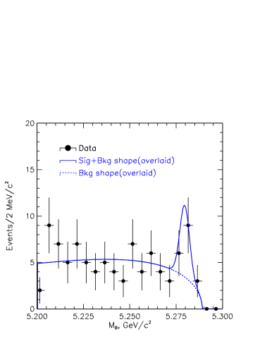
Figure 3: Distribution of $m_{\rm EC}$ obtained from the cut-based analysis using the NN. Superimposed on the data points are the signal and background $m_{\rm EC}$ distributions, normalized to the number of observed events.

The $m_{\rm EC}$ distribution of the events passing the selection requirements (except for the $m_{\rm EC}$ cut) is shown in Fig. 3 (for NN). For illustration purposes, we have superimposed the Gaussian signal contribution and the ARGUS background contribution; both distributions are normalized to the results given in Table 3.

3.4 Maximum Likelihood Analysis

The likelihood $P({f},x_{i})$ for event $\{i\}$ with a measured set of discriminating variables $x_{i}$, and for a signal fraction ${f}$, is defined as

$$P({f},x_{i})={f}p_{s}(x_{i})+(1-{f})p_{b}(x_{i})~{}.$$ (3)

The $p_{s}(x_{i})$ ($p_{b}(x_{i})$) is the product of the normalized signal (background) probability density functions (PDF) of the individual variables entering the fit: namely, $m_{\rm EC}$, $\Delta E$, $m(\eta)$ and the NN or Fisher output. The $\eta\pi$ invariant mass is not included since the line shape of the $a_{0}$ resonance is not well known at present [3]. The data sample is selected within generous sidebands for the variables that enter the fit (c.f. Sec. 3.1).

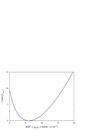
Figure 4: Negative log-likelihood function versus the signal branching fraction.

The signal distributions are obtained from Monte Carlo simulation, refined with data from the signal-like charmed $B$ decay mode $D\rho$, and inclusive samples. On-peak sideband events, controlled by off-peak data, are used to infer the corresponding background shapes. Multi-Gaussian, polynomial functions and cubic splines have been used to empirically approximate the reconstructed shapes of the discriminating variables.

After applying the event selection described in Sec. 3.1, a total of ${\cal N}=9248$ candidate events without multiple combinations enters the ML fit, corresponding to a signal efficiency of 32.8%. The fit is performed by minimizing the sum

$$-2\ln{\cal L}_{{f}}=-2\sum_{i=1}^{{\cal N}}\ln P({f},x_{i})~{},$$ (4)

over ${\cal N}$ events, with respect to the signal fraction ${f}$. The fit results in $N_{s}={f}{\cal N}=18.1_{\,-7.4}^{\,+8.7}$ signal events for NN, and $N_{s}=16.2_{\,-7.2}^{\,+8.6}$ signal events for Fisher. In the following, we restrict the discussion to the results obtained with the NN, since it provides the best signal efficiency. This choice has been made prior to uncovering the results. The negative log-likelihood function versus the signal branching fraction is depicted in Fig. 4. A “toy” Monte Carlo simulation indicates a goodness-of-fit of 50%. If the observed signal excess is interpreted as evidence for a signal, the corresponding branching fraction is

$${{\cal B}}(B^{0}\rightarrow a_{0}^{\pm}(a_{0}^{\pm}\rightarrow\eta\pi^{\pm})\pi^{\mp})\,=\,(6.2_{\,-2.5}^{\,+3.0}\pm 1.1)\times 10^{-6}~{},$$ (5)

where the first error quoted is statistical and the second is systematic. The statistical significance of this result corresponds to $3.7$ standard deviations. The latter is computed using a zero-signal toy Monte Carlo simulation. Systematic effects are discussed in Sec. 4. Assuming no evidence for a signal, the $90\%$ CL upper limit on the branching fraction, obtained from the integral $\int_{0}^{{\cal B}}{\cal L}_{{f}}({{\cal B}}^{\prime})d{{\cal B}}^{\prime}/\int_{0}^{\infty}{\cal L}_{{f}}({{\cal B}}^{\prime})d{{\cal B}}^{\prime}=0.9$, is

$${{\cal B}}(B^{0}\rightarrow a_{0}^{\pm}(a_{0}^{\pm}\rightarrow\eta\pi^{\pm})\pi^{\mp})<11.5\times 10^{-6}~{},$$ (6)

where the systematic uncertainty has been added linearly. A 65% correlation between the ML fit result (5) and the cut-based result (see Table 3) is found with a toy Monte Carlo simulation. The probability for finding a larger difference than that observed ($1.6\times 10^{-6}$) is found to be 54%.

The signal yield of the likelihood function can be displayed with the x-variable, defined by

$$x\,=\,\frac{p_{s}-p_{b}}{p_{s}+p_{b}}~{}.$$ (7)

Its distribution for the data sample used in the ML fit is shown by the points with error bars in the left-hand plots of Fig. 5. Also shown are the expectations from signal Monte Carlo (cross-hatched area), normalized to the signal yield of the ML fit, and background from on-peak sidebands (shaded area). A signal excess and good agreement between data and simulation are observed.

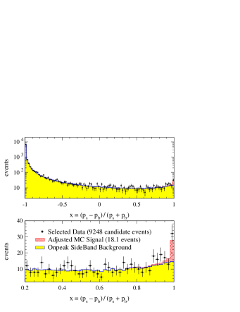
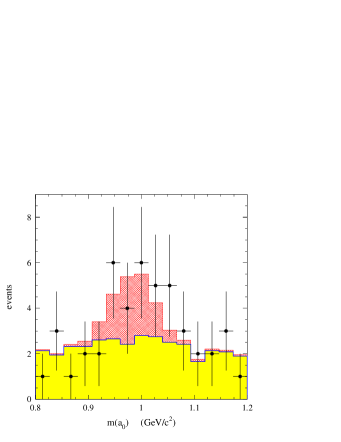
Figure 5: Left-hand plot: distributions of the $x$ variable (7) for data (points with error bars), signal Monte Carlo (cross-hatched area) and the background expectation from on-peak sidebands (shaded area). The signal region has been expanded in the lower plot. The simulated signal contribution is normalized to the ML fit result. A signal excess is observed. Right-hand plot: projection on the $\eta\pi$ invariant mass axis after requiring $x>0.98$, removing $44\%$ of the signal and 99.9% of the background.

Since the information from the shape of the $\eta\pi$ invariant mass distribution is not exploited in the likelihood function, one can use projections in order to verify that the signal candidates are consistent with the $a_{0}$ hypothesis. We select events with $x>0.98$, keeping $56\%$ of the signal while retaining only 0.1% of the background. The distributions of the corresponding data events, as well as the signal and background expectations are shown in Fig. 5. The data are consistent with the expected enhancement at the $a_{0}$ invariant mass.

4 Systematic Uncertainties

The main sources of systematic uncertainty originate from the accuracy of the simulation for the reconstruction of neutrals, from the tracking efficiency and from particle identification. Dedicated studies provide estimates of these effects. A $5\%$ uncertainty is assigned to the $\eta$ reconstruction efficiency, which represents the dominant error on the selection efficiency. The tracking efficiency difference between data and Monte Carlo simulation amounts to $3.9\%$. An uncertainty of $1.8\%$ is assigned due to particle identification.

Other systematics may arise from the imperfect simulation of the distributions of the discriminating variables. They have been studied with control samples. The widths and central values of the $\Delta E$ and $m_{\rm EC}$ signal distributions are calibrated with $B^{-}\rightarrow D^{0}(\rightarrow K^{-}\pi^{+})\rho^{-}$ decays, where the estimate of systematics using final states with $\pi^{0}$’s is expected to be conservative since the $\pi^{0}$’s have more combinatorial background than $\eta$’s. The $\eta$ and $a_{0}$ invariant mass distributions have been studied with inclusive data samples. Since the line shape of the $a_{0}$ resonance is not well known [3], we have used a generous mass window (c.f. Sec. 3.1) so that the resulting systematic effect from the $\eta\pi$ mass requirement is small. The Fisher and NN distributions have been checked by comparing on-peak sideband data and $q\overline{q}$ Monte Carlo, where all differences are assigned as systematic errors. The uncertainty on the signal efficiency related to the limited Monte Carlo statistics is negligible.

The contamination from continuum background in the cut-based analysis is evaluated by extrapolating the number of events found in the GSB, using the known shapes of the $\Delta E$ and $m_{\rm EC}$ background distributions. The consistency of the parameterizations has been checked for different regions of the sidebands, and between data sidebands and $q\bar{q}$ Monte Carlo samples as well as off-peak data. Good agreement is found. Associated uncertainties are estimated by varying the shape parameters within their statistical accuracies. The same procedure has been applied to estimate the systematic uncertainties from the cuts on the event shape variables and the MVA discriminants.

The estimate of the (mostly charmless) $B$-background has been performed with generic charmless Monte Carlo. We expect a contamination of $0.3$ events from non-resonant $\pi^{+}\pi^{-}\pi^{0}$ decays. The feedthrough from the unknown decay mode $B^{0}\rightarrow a_{0}^{+}K^{-}$ is determined from the comparison of the inclusive $a_{0}^{+}h^{-}$ signal yield (i.e., obtained without PID requirements) with the exclusive results of the cut-based analysis. No indication for a possible contamination from $a_{0}^{+}K^{-}$ events is found. A conservative 5% systematic is assigned to the kaon fraction in the $a_{0}^{+}\pi^{-}$ signal.

Table 4 summarizes the relative systematic errors used for the cut-based analysis. Where they differ, uncertainties are given separately for NN and Fisher.

Systematic effects specific to the ML analysis arise from differences in the background shapes of the MVA variables between data and Monte Carlo simulation ($15\%$). The systematic uncertainty from the correlations between the discriminating variables entering the fit, in particular those between the signal distributions of $\Delta E$ and $m_{\rm EC}$, amounts to $2\%$. The total systematic error for the ML fit is $18\%$.

Table 4: Summary of systematic uncertainties for the cut-based analysis.

Source	Uncertainty
$\eta$ finding	$5.0\%$
$\eta$ mass and resolution	$0.7\%$
$a_{0}$ mass and width/resolution	$0.1\%$
Track finding	$3.9\%$
PID	$2.6\%$
$\Delta E$	$1.7\%$
$m_{\rm EC}$	$0.1\%$
$\theta_{\rm T}$ and $\theta_{\rm TP}$	$1.0\%$
MVAs	NN: $1.0\%$, FI: $2.0\%$
GSB $q\bar{q}$ background estimate	NN: $1.3$ events, FI: $1.5$ events
Charmless $B$ background	$0.3$ events
$a_{0}^{+}K^{-}$ feedthrough	$5\%$
MC sample statistics	$0.2\%$
$B$ counting	$1.5\%$
Total error on branching fraction	NN: $15.7\%$, FI: $17.0\%$

5 Conclusions

The preliminary analysis reported in this paper shows an excess over expected background of $B^{0}\rightarrow a_{0}^{+}(980)\pi^{-}$ events, excluding the zero-signal hypothesis at the level of $3.7$ standard deviations. Interpreted as evidence for a signal, the excess would result in the branching fraction ${{\cal B}}(B^{0}\rightarrow a_{0}^{+}(a_{0}^{+}\rightarrow\eta\pi^{+})\pi^{-})=(6.2_{\,-2.5}^{\,+3.0}\pm 1.1)\times 10^{-6}$, where the first error quoted is statistical and the second is systematic. This corresponds to an upper limit of ${{\cal B}}(B^{0}\rightarrow a_{0}^{+}(a_{0}^{+}\rightarrow\eta\pi^{+})\pi^{-})<11.5\times 10^{-6}$ at 90% CL. We emphasize the use of improved, linear and non-linear multivariate background suppression techniques and optimal signal extraction criteria for rare decay searches.

Acknowledgements

We are grateful for the extraordinary contributions of our PEP-II colleagues in achieving the excellent luminosity and machine conditions that have made this work possible. The collaborating institutions wish to thank SLAC for its support and the kind hospitality extended to them. This work is supported by the US Department of Energy and National Science Foundation, the Natural Sciences and Engineering Research Council (Canada), Institute of High Energy Physics (China), the Commissariat à l’Energie Atomique and Institut National de Physique Nucléaire et de Physique des Particules (France), the Bundesministerium für Bildung und Forschung (Germany), the Istituto Nazionale di Fisica Nucleare (Italy), the Research Council of Norway, the Ministry of Science and Technology of the Russian Federation, and the Particle Physics and Astronomy Research Council (United Kingdom). Individuals have received support from the Swiss National Science Foundation, the A. P. Sloan Foundation, the Research Corporation, and the Alexander von Humboldt Foundation.

Appendix: Cut Optimization

The cut on the MVA variable output $x_{\rm out}$ (the final cut being denoted $x_{\rm out}^{\rm cut}$) is applied following a criterion designed for rare decay searches. In particular, it does not require one to know (or guess) the branching fraction of the signal one is looking for. When searching for a rare signal, one wants to rule out the null hypothesis: “there is no signal in the data sample”. For this purpose, one defines the confidence level

$${\rm CL}(N,x_{\rm out}^{\rm cut})=\sum_{n=N}^{\infty}{\cal P}_{n}(N_{b})~{},$$ (8)

where $N$ is the number of events retained by the final cut, $N_{b}$ is the expected number of background events passing the final cut, and ${\cal P}_{n}(N_{b})$ is the corresponding Poisson probability distribution. If ${\rm CL}$ is below a certain threshold (e.g., $5\%$, meaning that the hypothesis is excluded at $95\%$ ${\rm CL}$), one excludes the absence of rare decays, to this level. The idea is to adjust $x_{\rm out}^{\rm cut}$, hence varying both signal and background efficiencies to reach the lowest confidence level, on average.

Cut Optimization for Known Branching Fraction $\cal B$.

First, if the branching fraction is known, then, for a given $x_{\rm out}^{\rm cut}$, one can predict the expected number of $N_{s}$ signal events. The expected value of the ${\rm CL}$ of Eq. 8 (i.e., the average over a large number of hypothetical experiments) is

$$\langle{\rm CL}\rangle(x_{\rm out}^{\rm cut})=\sum_{N=0}^{\infty}{\cal P}_{N}(N_{s}+N_{b})\ {\rm CL}(N,x_{\rm out}^{\rm cut})~{}.$$ (9)

The optimal cut on $x_{\rm out}$, denoted $x_{\rm out}^{\rm opt}({{\cal B}})$, is the one which minimizes the above average, i.e., which leads to the clearest

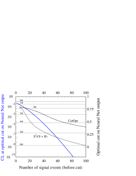
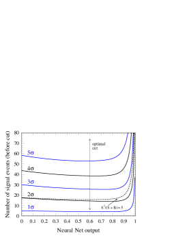
Figure 6: Left-hand plot: expected confidence levels and optimal cuts on the NN discriminant for an analysis where the branching fraction is known. The solid line gives the confidence level, obtained when using the optimal cut, as a function of the number of signal events (before cut). The dashed line is the optimal cut for a given number of events, and the dotted line gives the optimal cut using the criterion $S^{2}/(S+B)$. Right-hand plot: average number of signal events before NN cut, needed in the data sample to attain a given confidence level, on the average. Shown are the curves corresponding to $1\dots 5\sigma$. The minima of the curves correspond to the optimal cuts at a given significance level. Notice that the optimal cuts are approximately independent of the branching fraction. Shown in addition is the curve obtained for the constant signal excess $S^{2}/(S+B)=5$, corresponding to a significance of 2 standard deviations.

rejection of the (wrong) hypothesis:“there is no signal in the data sample”

$$\langle{\rm CL}\rangle(x_{\rm out}^{\rm opt}({{\cal B}}))=\langle{\rm CL}\rangle_{{\rm min};\,x_{\rm out}^{\rm cut}}(x_{\rm out}^{\rm cut})~{}.$$ (10)

Figure 6 (left hand plot) shows the confidence level achievable for a given number of expected signal events. Also shown are the variations of the optimal cut and the cut obtained when using the Gaussian criterion $S^{2}/(S+B)$ for optimization.

Cut Optimization for Unknown Branching Fraction.

When no expectation for the signal branching fraction is available, Eq. 10 cannot be used to define the optimal cut value of $x_{\rm out}^{\rm cut}$. The idea is then to replace the target branching fraction by a target confidence level. One chooses a particular value for the target ${\rm CL}$ (denoted ${\rm CL}^{\rm cut}$) one is aiming at to define the optimal $x_{\rm out}^{\rm cut}$ value as the value $x_{\rm out}^{\rm opt}$ (now without $({{\cal B}})$ as an argument) for which the equality

$$\langle{\rm CL}\rangle(x_{\rm out}^{\rm opt})={\rm CL}^{\rm cut}~{},$$ (11)

is reached for the smallest $\cal B$. In the following we use ${\rm CL}^{\rm cut}=0.05$. The performance for unknown branching fraction is illustrated for the NN discriminant in the right hand plot of Fig. 6.

References

- [1] A.S. Dighe, C.S. Kim , Phys.Rev.D62, 111302 (2000).
- [2] S. Laplace and V. Shelkov, “CP Violation and the Absence of Second Class Currents in Charmless B Decays”, LAL 01-24, LBNL-47757, hep-ph/0105252 (2001), to appear in Eur. Phys. J. C.
- [3] Particle Data Group, D.E. Groom et al., Eur. Phys. Jour. C 15, 1 (2000).
- [4] BABAR Collaboration, B. Aubert et al., “The BABAR Detector”, hep-ex/0105044 (2001), to appear in Nucl. Instr. and Meth..
- [5] P. Gay, B. Michel, J. Proriol, and O. Deschamps, “Tagging Higgs Bosons in Hadronic LEP-2 Events with Neural Networks.”, In Pisa 1995, New computing techniques in physics research, 725 (1995).
- [6] BABAR Collaboration, P.F. Harrison and H.R. Quinn, eds., “The BABAR Physics Book”, SLAC-R-504 (1998).
- [7] CLEO Collaboration, D.M. Asner et al., Phys. Rev. D53, 1039 (1996).
- [8] ARGUS Collaboration, H. Albrecht et al., Phys. Lett. B185, 218 (1987); B241, 278 (1990).