Energy Spectra, Altitude Profiles and Charge Ratios of Atmospheric Muons

Abstract

We present a new measurement of air shower muons made during atmospheric ascent of the High Energy Antimatter Telescope balloon experiment. The muon charge ratio $\mu^{+}/\mu^{-}$ is presented as a function of atmospheric depth in the momentum interval 0.3–0.9 GeV/c. The differential $\mu^{-}$ momentum spectra are presented between 0.3 and $\sim$50 GeV/c at atmospheric depths between 13 and 960 g/cm². We compare our measurements with other recent data and with Monte Carlo calculations of the same type as those used in predicting atmospheric neutrino fluxes. We find that our measured $\mu^{-}$ fluxes are smaller than the predictions by as much as 70% at shallow atmospheric depths, by $\sim$20% at the depth of shower maximum, and are in good agreement with the predictions at greater depths. We explore the consequences of this on the question of atmospheric neutrino production.

I Introduction

Measurements of the flux of atmospheric neutrinos by large underground detectors have consistently disagreed with theoretical predictions, a fact that has been interpreted in terms of possible neutrino oscillations. The most compelling evidence thus far comes from the SuperKamiokande experiment [1]. The discrepancies between experiment and theory are well beyond the statistical uncertainties in the measurements. The correct interpretation of the effect requires a detailed understanding of neutrino production in the atmosphere.

Model predictions [2, 3, 4, 5, 6] of the absolute flux of neutrinos produced in air showers are uncertain due to a number of difficulties: one problem is the normalization of the primary cosmic-ray flux, for which measurements vary by $\pm$15% or more. Because of this, different assumptions are made by different authors. For instance, the model of Honda et al. [4], used as the starting point in the analyses of the SuperKamiokande collaboration, assumes a primary cosmic ray flux normalization that is in excess of the current measurements by balloon experiments [7], by as much as $\sim$20% in the energy range beyond about 5 GeV, which is relevant to the production of sub- to multi-GeV atmospheric neutrinos. In contrast, the model of the Bartol group [6, 8] uses a primary spectrum in good agreement with the most recent measurements. Different assumptions are also made about the details of particle production in atmospheric interactions, and about the treatment of geomagnetic effects (see Ref. [9]). Thus, while the authors of these calculations expect that the predictions of absolute neutrino fluxes might have a total uncertainty of about 18% [6], it seems fortuitous that the predicted neutrino rates have been found to agree with each other within about 10%. It should also be noted that in the neutrino oscillation analysis of the SuperKamiokande collaboration, an additional normalization factor of 1.16 in the cosmic ray intensity is introduced to obtain the best oscillation fit to the measured muon and electron neutrino rates as a function of zenith angle.

Neutrino production in the atmosphere is closely coupled to muon production, as both types of particles are produced together in pion and kaon decays, and as some of the muons decay to produce further neutrinos. Monte Carlo simulations of neutrino production naturally predict the spectra of muons as a function of atmospheric depth. Therefore, a detailed experimental test of the predictions is possible through measurements of the intensity of muons at different depths in the atmosphere, for instance with a balloon-borne particle detector during atmospheric ascent. If such a detector includes a magnet spectrometer, separate measurements of the $\mu^{-}$ and $\mu^{+}$ fluxes are possible. This is relatively easy for negative muons, as negatively charged particles other than electrons are rare in air showers (and electrons are easily rejected), while non-interacting protons generate a large background for positive muons above $\sim$1 GeV. Such measurements have been made by a number of instruments, including the MASS [10, 11], HEAT [12, 13], CAPRICE [14], and IMAX [15] magnet spectrometers and older, less sensitive balloon payloads.

Here we describe measurements made with the High Energy Antimatter Telescope (HEAT), a balloon instrument optimized for the study of high-energy cosmic-ray electrons and positrons. HEAT uses several complementary particle identification techniques, which are also well suited to the identification of muons during atmospheric ascent of the balloon. This instrument was flown twice, in 1994 and 1995. Preliminary results from the first flight on relative abundances of $\mu^{+}$ and $\mu^{-}$ were reported previously [12]. The present paper describes measurements made during the second balloon flight: the relative abundances of $\mu^{+}$ and $\mu^{-}$ at momenta between 0.3 and 0.9 GeV/c, and the differential spectra of $\mu^{-}$ at momenta between 0.3 and 50 GeV/c, at atmospheric depths between 13 and 960 g/cm². We compare the results with other measurements and with calculations made with a modified version of the TARGET Monte Carlo algorithm [6], developed by the Bartol group to predict atmospheric neutrino rates.

II Muon Identification and Backgrounds

The HEAT instrument is described in detail elsewhere [16]. It combines a superconducting magnet spectrometer (using a drift-tube tracking hodoscope), a time-of-flight (TOF) system, a transition-radiation detector (TRD) and an electromagnetic calorimeter (EMC). For its second flight, it was launched from Lynn Lake, Manitoba, Canada, at a vertical geomagnetic cutoff rigidity of well below 1 GV. The flight took place on 23 August 1995, approximately at minimum solar activity. The ascent from an atmospheric overburden at the ground of 960 g/cm² to a float altitude at 3 g/cm² required 3.1 hours, during which charged atmospheric secondary particles were detected and recorded. Near the end of ascent, at about 13 g/cm², the instrument trigger configuration was changed to commence preferential measurements of electrons and positrons, affecting the ability to measure absolute muon intensities at shallower depths. Therefore we report measurements of the muon charge ratio at all atmospheric depths, but measurements of absolute muon intensities only at depths greater than 13 g/cm².

In identifying muon events, TRD information is not used. The TOF system measures the velocity of the particle $\beta=v/c$ with a resolution of $\sigma_{\beta}=0.15$, permitting complete rejection of upward-going particles; in addition, the amount of light generated in the scintillation counters of the TOF system is used to measure the magnitude of the particle’s electric charge $Ze$ with a resolution of $\sigma_{Z}=0.11$, permitting the unambiguous identification of singly-charged particles. The magnet spectrometer measures the sign of the particle’s charge from the direction of the deflection in a magnetic field of about 1 T, with a field integral over the particle’s trajectory of $\int B\cdot dl\sim 4.2$ kGm. The magnetic rigidity $R=pc/Ze$ of the particle is determined from the amount of deflection; at rigidities between 0.3 and 0.9 GV, the resolution achieved is $\sigma_{R}=0.08$ to 0.11 GV. The EMC records the pattern of energy deposits in 10 scintillation counters, each topped by a 0.9 radiation length-thick lead sheet. In each layer, the energy deposited is measured in units of the energy loss by a vertical minimum-ionizing particle (MIP). A shower sum is obtained by adding the signals from the 10 scintillators.

The selection of muon events proceeds in three steps. First, a high-quality spectrometer track and measurement of the rigidity $R$ are required, as described in Ref. [13]. Also required are down-going and singly-charged TOF characteristics. Second, as shown in Figure 1, the distribution of reconstructed particle rigidity $R$ is studied as a function of velocity $\beta$, and compared with ideal curves $R=(m/Z)\beta/\sqrt{(1-\beta^{2})}$ where $m$ is the mass and $Z$ the charge of the particle. Clearly identifiable in the figure are populations due to He (and d), p, $\mu^{+}$ and $\mu^{-}$ events. $\pi^{\pm}$ and some $K^{\pm}$ events cannot be distinguished from the $\mu^{\pm}$ populations, and are a small background to the muon signal. We select $\mu$-like events by requiring: 1) $\beta\geq 0.85$ and 2) $0.3\leq\left|R\right|\leq 0.9$ GV, for the low-energy $\mu^{+}/\mu^{-}$ ratio, and 2) $R\leq-0.3$ GV for the $\mu^{-}$ energy spectra. For $R\geq 0.9$ GV, $\mu^{+}$ events become indistinguishable from non-showering hadrons (mostly protons), so that $\mu^{+}$ spectra are not measured with this instrument. Third, we study the behavior of the shower sum measured by the EMC as a function of particle rigidity $R$, as shown in Figure 2. Ideal curves for electrons and positrons are obtained by assuming a simple linear relationship between EMC sum (proportional to energy) and $R$. For heavier particles, a calculation of EMC sum is made by integrating Bethe-Bloch energy losses within the EMC scintillators. Populations of events due to e^±, p and $\mu^{\pm}/\pi^{\pm}/K^{\pm}$ are identifiable. By augmenting the selection criteria of Figure 1 with the requirement that particles not shower in the EMC (EMC sum $\leq$ 15), e^± events with $\left|R\right|>0.3$ GV are rejected. The low-rigidity proton events that range out in the EMC and would appear to contaminate the $\mu^{+}$ population are rejected by the $\beta\geq 0.85$ requirement of Figure 1.

With these criteria, we achieve essentially complete rejection of electron events, but there remains a small background to the muon signal due to pions and kaons. We estimate from Monte Carlo simulations of air showers based on CERN’s GEANT-FLUKA algorithms [17] that the $\pi^{\pm}$ flux at a depth of 13 g/cm² is only 2% that of $\mu^{\pm}$, in agreement with another calculation [18] – with $K^{\pm}$ fluxes at a much lower level – and that this further decreases with increasing atmospheric depth. Moreover, only pions that do not interact can be mistaken for muons, which occurs 39% of the time, so that the background to the muon measurement due to atmospheric pions is only about 0.7-0.9% near float, decreasing to less than 0.4% at depths greater than 300 g/cm². Such a small background is not corrected for here. Occasionally, cosmic-ray interactions in the instrument result in $\pi^{\pm}$ production, at an even more modest level than the atmospheric pion background. GEANT-based simulations indicate that only 0.04% of proton-induced events yield a misidentification as a $\mu^{-}$. As the payload slowly rotated throughout the flight (as determined with a solar sensor attached outside the gondola), and did not align itself with the Earth’s magnetic field, possible geomagnetic East-West asymmetries are averaged out. Furthermore, such asymmetries in the primary proton flux are only expected at momenta near the geomagnetic cutoff, which for the Lynn Lake flight is well below the energies of interest here.

III Results and Discussion

A Muon Charge Ratio

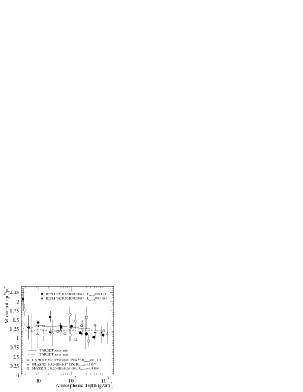
The number of low-energy $\mu^{+}$ and $\mu^{-}$ events detected as a function of atmospheric depth and the $\mu^{+}/\mu^{-}$ ratio are summarized in Table I. The $\mu^{+}/\mu^{-}$ ratio is shown as a function of atmospheric depth in Figure 3 (labeled HEAT 95), together with the measured ratio from the first HEAT flight [12] (labeled HEAT 94) and other recent measurements [14, 15, 19]. As noted on the figure, the various analyses have used different magnetic rigidity ranges, and moreover, the measurements were made at different solar epochs and different geomagnetic rigidity cutoffs R_cutoff, so that the data are not truly directly comparable. The two HEAT measurements of the muon ratio are the most statistically significant, and are essentially consistent with each other and with other measurements, within the appreciable errors. Based on the HEAT measurements, no clear correlation of the muon ratio with geomagnetic cutoff rigidity is observed. The depth dependence of the charge ratio seems to be essentially flat, although a slight decrease from about 1.3-1.4 at high altitudes (3-50 g/cm²) down to about 1.1 at the ground cannot be excluded. We note that the charge ratio measured by both HEAT 95 and CAPRICE 94 at small depths appears anomalously high. This effect is not understood at present. Also shown on Figure 3 are calculations with the TARGET algorithm [6] (widely used for neutrino flux calculations), for conditions of solar minimum and maximum activity. Both HEAT flights occurred under essentially solar-minimum conditions. The TARGET calculations have been made for average primary fluxes at solar minimum and maximum, which may not exactly represent the actual spectrum at the time of the flight. The calculations are for a location with no geomagnetic cutoff, and are intended for comparison with the HEAT 95 data only. The agreement between the HEAT measurements and the solar-minimum TARGET calculation appears to be fairly good. Note that the fluctuations in the simulated distributions at shallow atmospheric depths are statistical, and indicative of the small number of muons having been produced in the air showers at the highest altitudes.

B Energy Spectra of Negative Muons

The absolute intensity of $\mu^{-}$, in a rigidity interval $\Delta R$ with an average rigidity $\overline{R}$, at atmospheric depth $d$ is obtained with:

$$j_{\mu}(d,\overline{R})={N_{\mu}\over\Delta t\epsilon_{t}\epsilon_{l}\epsilon_{\theta}\epsilon_{dt}\Delta R(\Omega A)\epsilon_{scan}\epsilon_{acc}},$$

where $N_{\mu}$ is the number of $\mu^{-}$ events recorded at $(d,\overline{R})$, $\Delta t$ is the time spent at depth $d$, $\epsilon_{t}$ is the live time fraction, $\epsilon_{l}$ is an event-transmission loss correction, $\epsilon_{\theta}$ is a correction to account for the fact that the muon flux is increasingly less isotropic deeper in the atmosphere, $\epsilon_{dt}$ is the efficiency of the basic event cleanliness criteria applied to the drift-tube hodoscope track, $(\Omega A)$ is the geometrical factor, $\epsilon_{scan}$ is a “scanning efficiency” correction (described below), and $\epsilon_{acc}$ is the muon acceptance efficiency. The acceptance of the instrument decreases rapidly for particles incident at a zenith angle greater than about 25^∘, so that particle intensities reported here are essentially for vertical incidence.

Both $\overline{R}$ and $\Delta R$ are weighted to account for the details of the energy spectrum, according to:

$$\overline{R}={\int_{R_{i}}^{R_{j}}Rf(R)dR\over\int_{R_{i}}^{R_{j}}f(R)dR}\;\;\;\;\;\;\Delta R={\int_{R_{i}}^{R_{j}}f(R)dR\over f(\overline{R})}$$

where $f(R)\propto R^{-\alpha}$ is the rigidity power-law spectrum, with spectral index $\alpha$ varying between $-0.56$ and 3.5 depending on both $R$ and $d$ ($\alpha$ is experimentally determined from the spectra before any of the normalization corrections are applied). $\Delta t$ is measured with an on-board clock, $\epsilon_{t}$ is determined using on-board scalers which count clock cycles while the instrument is available for a trigger or busy processing an event, and $\epsilon_{l}$ is determined by careful accounting of event numbers generated on board compared to events successfully transmitted. $\epsilon_{\theta}$ is calculated using a standard prescription [20], where the zenith dependence of the muon flux is taken to be $\cos^{n(d)}\theta$, with the exponent $n$ a function of atmospheric depth $d$; we have used $n(d)=(d/1030{\rm g/cm^{2}})\times n_{sealevel}$ with $n_{sealevel}=2$. $\epsilon_{dt}$ is obtained by a careful accounting of the number of events recorded compared to the number of events with a successful minimal track reconstruction. $(\Omega A)$ and $\epsilon_{acc}$ are determined with the aid of a GEANT-based simulation of the response of the HEAT instrument. $\epsilon_{scan}$ is a correction factor introduced based on the visual scanning of several hundred events to account for residual differences between the reconstruction efficiency of real events compared to that of simulated ones, and is found to be $\epsilon_{scan}=(0.9\pm 0.1)$. The various parameters described above are given in Tables II and III.

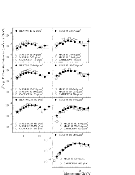
The final $\mu^{-}$ intensities as a function of momentum for various atmospheric depths are shown in Figure 4 and given in Table IV. Also shown in the figure are the measurements of the MASS [10, 11] and CAPRICE [14] experiments. The HEAT sample of 10327 $\mu^{-}$ events collected during ascent is to be compared with the MASS samples of 2893 events (1989 flight) and 4471 events (1991 flight) and the CAPRICE sample of 4627 events. Although the 1989 MASS measurements were also made in Northern Canada (from Prince Albert, Saskatchewan), the flight occurred at a different solar epoch (1989), at the time of a significant Forbush decrease. The 1991 MASS measurements were made from Fort Sumner, New Mexico. The CAPRICE data were collected at Lynn Lake, in 1994, and so are more directly comparable with our measurements. The general level of agreement between the data sets should be noted.

C Comparison with Model Calculations

1 One-Dimensional TARGET Algorithm

In Figure 5, we compare the HEAT measurements reported here with predictions of the TARGET algorithm [6], for conditions of solar minimum and maximum activity, shown as solid and dotted curves, respectively. (The solar-minimum curves are the ones of interest here, but the solar maximum curves are shown as well to illustrate the extent of the effect of the solar cycle on muon production.) These curves are obtained with the standard TARGET algorithm, which simulates vertically incident cosmic rays, and which follows the development of the air shower in one dimension only. No corrections for geomagnetic effects are made. This is the algorithm developed by the Bartol group and used in predicting underground neutrino rates from atmospheric sources [6, 8]. In Figure 6, we show the $\mu^{-}$ growth curves for different momentum intervals, also compared with the 1D TARGET-based predictions for solar minimum conditions (solid curves). The calculations were not made for the highest momentum bin.

There is general similarity between the experimental and simulated distributions, with some notable differences. For instance, the predictions are significantly in excess of the measurements below 4 GeV/c at atmospheric depths between 13 and 250 g/cm². The ratio of simulated to measured intensity varies from $1.2\pm 0.2$ near shower maximum at 200 g/cm² to $1.7\pm 0.3$ at depths between 13 and 140 g/cm². At depths beyond shower maximum, or at momenta greater than 4 GeV/c, the simulations agree very well with our measurements. A similar trend was found by the CAPRICE collaboration [14]: simulations predict more $\mu^{-}$ events than they measure below about 1 GeV/c, but they find that the ratio of simulated to measured intensity is greatest at shower maximum, with a value of $1.8\pm 0.1$.

2 Three-Dimensional TARGET Algorithm

In an attempt to understand the origin of the discrepancy between the predicted and measured muon intensities, a new version of the TARGET algorithm was produced in collaboration with T. Gaisser and T. Stanev of the Bartol Research Institute. In this, three dimensional air shower development effects are taken into account, and the primary cosmic ray arrival direction is sampled isotropically, rather than assuming vertical incidence. Geomagnetic effects are not yet included in the calculations. Figure 5 also shows the $\mu^{-}$ momentum spectra at various atmospheric depths obtained with the 3-dimensional TARGET algorithm (dashed curves), for solar minimum conditions. The 3D calculations are in substantially better agreement with the data than the 1D calculations. In Figure 6, the measured $\mu^{-}$ growth curves are also compared with 3D TARGET predictions (dashed curves). Here again the 3D predictions are a more adequate representation of the data.

Figure 7 shows distributions of the ratios of predicted to measured $\mu^{-}$ intensities, for 1D TARGET calculations (top panel) and 3D TARGET calculations (bottom panel), respectively. These are cumulative distributions for all momentum and atmospheric depth bins. Each ratio is weighted by the square of the error on the ratio derived from the experimental error on the intensity. The distribution for 1D calculations has a mean 1.13, indicating an average overprediction of 13%, whereas for 3D calculations the mean is 1.07, a slightly better agreement. The main improvement however is in the reduced RMS variance of 0.17 for the distribution for 3D calculations compared to 0.27 for the 1D calculations. Thus, the more realistic calculations that take into account 3D air shower development and primary zenith arrival direction constitute a clear improvement in the representation of muon production.

3 Neutrino Production

The 1D and 3D TARGET algorithms were used to predict ($\nu_{\mu}+{\overline{\nu}}_{\mu}$) and ($\nu_{\rm e}+{\overline{\nu}}_{\rm e}$) intensities at different atmospheric depths and in different momentum bins. The calculations are made for solar minimum conditions, for no geomagnetic rigidity cutoff, and for primary cosmic rays arriving within 30^∘ of the zenith. The resulting neutrino growth curves in different momentum intervals are shown in Figure 8. The calculations are made only up to 32 GeV/c. Although there are differences between the 1D and 3D predictions at momenta less than about 1 GeV/c, these differences are most important at mid-to-high altitudes. The neutrino intensities at the ground level, which are the ones of relevance to the underground neutrino studies, are summarized in Table V, for 1D and 3D calculations. The neutrino intensities at ground level appear not to be altered much by the 3D effects. A similar conclusion was also reached in a study by Battistoni et al. [21], where detailed calculations of atmospheric muon and neutrino production are made in one and three dimensions.

IV Conclusions

We have made statistically significant measurements of air shower muons as a function of atmospheric depth. We report the muon charge ratio $\mu^{+}/\mu^{-}$ in the momentum range 0.3-0.9 GeV/c and the momentum spectra of $\mu^{-}$ in the range 0.3-50 GeV/c, at atmospheric depths from 13 to 960 g/cm². The charge ratio is essentially constant with altitude within errors, with a possible decrease from 1.3-1.4 at high altitudes to 1.1 at the ground. A comparison of our measured $\mu^{-}$ momentum distributions with model calculations indicates significant discrepancies with the predictions of the standard one-dimensional TARGET algorithm: our measured fluxes are lower than the calculated ones at shallow depths before about shower maximum. Calculations of the muon intensities with a new version of the TARGET algorithm, accounting for three-dimensional air shower development, lead to a substantially improved agreement with our data. A detailed representation of atmospheric secondary production thus benefits from the more realistic simulations. The average excess of about 7% of the 3D calculations over our measured intensities is comparable to possible systematic effects in our experiment. Thus, within this uncertainty, the 3D TARGET algorithm generates atmospheric secondary particle intensities which are in agreement with the measurements.

The three-dimensional air shower development effects do not appear to impact significantly the atmospheric neutrino rates at the ground, but merely the pattern of neutrino production altitudes. Thus, we estimate that the neutrino intensities predicted by the 1D version of the TARGET algorithm are also accurate to about 7%. This is to be compared with the accuracy of 14-18% first estimated for such calculations [6]. Even though the Honda et al. [4] model uses different assumptions about the primary cosmic ray flux and about the atmospheric interaction characteristics, it predicts neutrino intensities on the ground which agree with the TARGET predictions and with our data at the level of 7-10%. Therefore, one might put into question the additional normalization factor of 1.16 of the primary cosmic ray spectrum that is introduced in the SuperKamiokande neutrino oscillation analysis.

FIG. 1.: Distribution of particle rigidity $R$ as a function of velocity $\beta=v/c$ for ascent data.

FIG. 2.: Distribution of shower sum in the EMC as a function of particle rigidity $R$ for ascent data.

FIG. 3.: Measured muon ratio $\mu^{+}/\mu^{-}$ as a function of atmospheric depth. The curves are calculations with the TARGET algorithm. The HEAT data are for $0.3\leq\left|R\right|\leq 0.9$ GV.

FIG. 4.: Differential $\mu^{-}$ momentum spectra as a function of atmospheric depth. The HEAT measurements are compared with the MASS and CAPRICE measurements for qualitative purposes only.

FIG. 5.: Differential $\mu^{-}$ momentum spectra measured by HEAT for various atmospheric depths. The curves are predictions of the 1D TARGET algorithm at solar minimum (solid curves) or solar maximum (dotted curves) conditions, and the 3D TARGET algorithm at solar minimum (dashed curves), respectively.

FIG. 6.: $\mu^{-}$ growth curves measured by HEAT for different momentum intervals. The curves are predictions of the 1D TARGET algorithm (solid curves) and 3D TARGET algorithm (dashed curves), respectively, for solar minimum conditions.

FIG. 7.: Distribution of the ratios of predicted to measured $\mu^{-}$ intensities, for 1D TARGET calculations (top panel) and 3D TARGET calculations (bottom panel), respectively. Each ratio is weighted by the square of the error on the ratio derived from the experimental error on the intensity.

FIG. 8.: $\nu$ growth curves predicted by TARGET at Lynn Lake, for solar minimum conditions, in different momentum intervals. The curves are: 1D $(\nu_{\mu}+{\overline{\nu}}_{\mu})$, solid curves; 3D $(\nu_{\mu}+{\overline{\nu}}_{\mu})$, dashed curves; 1D $(\nu_{\rm e}+{\overline{\nu}}_{\rm e})$, dotted curves; 3D $(\nu_{\rm e}+{\overline{\nu}}_{\rm e})$, dot-dashed curves.

.

TABLE I.: Muon counts at $0.3\leq\left|R\right|\leq 0.9$ GV as a function of atmospheric depth $d$. Uncertainties are statistical.

$d$	$\overline{d}$	N${}_{\mu^{+}}$	N${}_{\mu^{-}}$	$\mu^{+}/\mu^{-}$
(g/cm2)	(g/cm2)
3-4	3.45	134	65	$2.06\pm 0.31$
4-7	5.13	35	27	$1.30\pm 0.33$
7-13	9.85	53	37	$1.43\pm 0.31$
13-32	23.2	305	193	$1.58\pm 0.15$
32-67	49.1	458	348	$1.316\pm 0.094$
67-140	105	1264	954	$1.325\pm 0.057$
140-250	190	1691	1463	$1.156\pm 0.041$
250-350	298	605	540	$1.120\pm 0.066$
350-840	499	810	792	$1.023\pm 0.051$
840-960	957	1076	990	$1.087\pm 0.048$

TABLE II.: Rigidity-dependent parameters and corrections used in the determination of the absolute $\mu^{-}$ intensities.

$R$	$\overline{R}$	$\epsilon_{dt}$	$(\Omega A)$	$\epsilon_{acc}$
(GV)	(GV)	(%)	(cm2sr)	(%)
0.3-0.5	0.40	68.35$\pm$0.22	568.9$\pm$2.6	52.0$\pm$0.5
0.5-0.8	0.65	74.46$\pm$0.20	613.1$\pm$2.8	63.0$\pm$0.5
0.8-1.2	0.99	78.77$\pm$0.19	608.2$\pm$2.7	66.1$\pm$0.5
1.2-1.7	1.43	80.46$\pm$0.18	604.4$\pm$2.7	65.4$\pm$0.5
1.7-2.5	2.06	81.57$\pm$0.18	600.0$\pm$2.7	64.6$\pm$0.5
2.5-4	3.13	81.64$\pm$0.18	601.9$\pm$2.7	63.9$\pm$0.5
4-8	5.52	81.48$\pm$0.18	598.9$\pm$2.7	62.5$\pm$0.5
8-16	11.0	81.45$\pm$0.18	603.6$\pm$2.7	61.2$\pm$0.5
16-32	21.3	81.45$\pm$0.18	606.0$\pm$2.7	47.0$\pm$0.4
32-50	39.2	81.43$\pm$0.18	602.4$\pm$2.7	15.5$\pm$0.2

TABLE III.: Depth-dependent parameters and corrections used in the determination of the absolute $\mu^{-}$ intensities.

$d$	$\overline{d}$	$\Delta t$	$\epsilon_{t}$	$\epsilon_{l}$	$\epsilon_{\theta}$
(g/cm2)	(g/cm2)	($\pm 1$ s)	(%)	(%)	(%)
13-32	23.2	1453	48.1$\pm$1.8	89.190$\pm$0.079	99.68
32-67	49.1	1307	41.9$\pm$1.6	96.585$\pm$0.047	99.33
67-140	105	1571	49.5$\pm$4.6	95.051$\pm$0.051	98.58
140-250	190	1285	65.8$\pm$6.9	92.894$\pm$0.072	97.45
250-350	298	484	82.9$\pm$0.3	95.45$\pm$0.12	96.05
350-840	499	1163	95.7$\pm$0.2	94.30$\pm$0.14	93.50
840-960	957	5335	99.3$\pm$0.1	97.09$\pm$0.10	88.03

.

TABLE IV.: Number of recorded $\mu^{-}$ events and their intensity (in (cm²s sr GeV/c)^-1) as a function of momentum and atmospheric depth.

	0.40 GeV/c	0.65 GeV/c	0.99 GeV/c	1.43 GeV/c	2.06 GeV/c
23.2	81	86	89	42	51
g/cm2	$(4.12\pm 0.67)\times 10^{-3}$	$(2.06\pm 0.33)\times 10^{-3}$	$(1.45\pm 0.23)\times 10^{-3}$	$(5.5\pm 1.1)\times 10^{-4}$	$(4.22\pm 0.77)\times 10^{-4}$
49.1	135	181	100	97	90
g/cm2	$(6.7\pm 1.0)\times 10^{-3}$	$(4.42\pm 0.62)\times 10^{-3}$	$(1.68\pm 0.26)\times 10^{-3}$	$(1.29\pm 0.20)\times 10^{-3}$	$(7.6\pm 1.2)\times 10^{-4}$
105	354	494	403	285	241
g/cm2	$(1.32\pm 0.20)\times 10^{-2}$	$(8.7\pm 1.3)\times 10^{-3}$	$(4.86\pm 0.75)\times 10^{-3}$	$(2.74\pm 0.43)\times 10^{-3}$	$(1.46\pm 0.23)\times 10^{-3}$
190	568	721	626	441	370
g/cm2	$(2.02\pm 0.32)\times 10^{-2}$	$(1.21\pm 0.19)\times 10^{-2}$	$(7.2\pm 1.1)\times 10^{-3}$	$(4.03\pm 0.65)\times 10^{-3}$	$(2.13\pm 0.34)\times 10^{-3}$
298	198	268	245	191	189
g/cm2	$(1.47\pm 0.20)\times 10^{-2}$	$(9.4\pm 1.3)\times 10^{-3}$	$(5.84\pm 0.79)\times 10^{-3}$	$(3.63\pm 0.51)\times 10^{-3}$	$(2.26\pm 0.31)\times 10^{-3}$
499	235	441	398	309	275
g/cm2	$(6.68\pm 0.89)\times 10^{-3}$	$(5.83\pm 0.73)\times 10^{-3}$	$(3.56\pm 0.45)\times 10^{-3}$	$(2.21\pm 0.29)\times 10^{-3}$	$(1.23\pm 0.16)\times 10^{-3}$
957	280	550	624	630	653
g/cm2	$(1.85\pm 0.23)\times 10^{-3}$	$(1.61\pm 0.19)\times 10^{-3}$	$(1.22\pm 0.14)\times 10^{-3}$	$(9.8\pm 1.2)\times 10^{-4}$	$(6.36\pm 0.75)\times 10^{-4}$

	3.13 GeV/c	5.52 GeV/c	11.0 GeV/c	21.3 GeV/c	39.2 GeV/c
23.2	34	23	7	4	0
g/cm2	$(1.52\pm 0.32)\times 10^{-4}$	$(4.04\pm 0.97)\times 10^{-5}$	$(6.5\pm 2.6)\times 10^{-6}$	$(2.4\pm 1.2)\times 10^{-6}$
49.1	62	44	22	4	1
g/cm2	$(2.80\pm 0.49)\times 10^{-4}$	$(8.0\pm 1.5)\times 10^{-5}$	$(2.02\pm 0.49)\times 10^{-5}$	$(2.6\pm 1.3)\times 10^{-6}$	$(1.8\pm 1.8)\times 10^{-6}$
105	173	128	44	12	3
g/cm2	$(5.73\pm 0.94)\times 10^{-4}$	$(1.68\pm 0.29)\times 10^{-4}$	$(2.93\pm 0.61)\times 10^{-5}$	$(5.3\pm 1.7)\times 10^{-6}$	$(3.6\pm 2.1)\times 10^{-6}$
190	276	216	77	14	2
g/cm2	$(8.7\pm 1.4)\times 10^{-4}$	$(2.69\pm 0.45)\times 10^{-4}$	$(4.86\pm 0.93)\times 10^{-5}$	$(6.3\pm 1.9)\times 10^{-6}$	$(2.7\pm 1.9)\times 10^{-6}$
298	151	126	40	10	2
g/cm2	$(9.9\pm 1.4)\times 10^{-4}$	$(3.25\pm 0.48)\times 10^{-4}$	$(5.2\pm 1.0)\times 10^{-5}$	$(8.8\pm 3.0)\times 10^{-6}$	$(4.9\pm 3.5)\times 10^{-6}$
499	272	247	95	30	4
g/cm2	$(6.61\pm 0.87)\times 10^{-4}$	$(2.35\pm 0.31)\times 10^{-4}$	$(4.57\pm 0.71)\times 10^{-5}$	$(9.9\pm 2.1)\times 10^{-6}$	$(3.5\pm 1.8)\times 10^{-6}$
957	723	735	380	124	13
g/cm2	$(3.79\pm 0.45)\times 10^{-4}$	$(1.49\pm 0.17)\times 10^{-4}$	$(4.11\pm 0.50)\times 10^{-5}$	$(8.6\pm 1.2)\times 10^{-6}$	$(2.34\pm 0.70)\times 10^{-6}$

TABLE V.: Near vertical neutrino intensities at 960 g/cm² at zero geomagnetic cutoff, for 1D and 3D TARGET calculations. All intensities are in (cm² s sr GeV/c)^-1.

Momentum	$(\nu_{\mu}+{\overline{\nu}}_{\mu})$	$(\nu_{\mu}+{\overline{\nu}}_{\mu})$	$(\nu_{\rm e}+{\overline{\nu}}_{\rm e})$	$(\nu_{\rm e}+{\overline{\nu}}_{\rm e})$
(GeV/c)	1D Intensity	3D Intensity	1D Intensity	3D Intensity
0.36	0.32	0.31	0.15	0.14
0.71	0.063	0.062	0.027	0.026
0.89	0.035	0.035	0.014	0.014
1.4	0.0099	0.0099	0.0038	0.0038
1.8	0.0051	0.0052	0.0019	0.0019
2.8	0.0014	0.0014	$4.1\times 10^{-4}$	$4.3\times 10^{-4}$
5.6	$1.8\times 10^{-4}$	$1.8\times 10^{-4}$	$4.0\times 10^{-5}$	$4.2\times 10^{-5}$
11	$2.3\times 10^{-5}$	$2.3\times 10^{-5}$	$3.7\times 10^{-6}$	$3.6\times 10^{-6}$
22	$2.6\times 10^{-6}$	$2.6\times 10^{-6}$	$2.9\times 10^{-7}$	$3.0\times 10^{-7}$