Confronting classical and Bayesian confidence limits to examples

Abstract

Classical confidence limits are compared to Bayesian error bounds by studying relevant examples. The performance of the two methods is investigated relative to the properties coherence, precision, bias, universality, simplicity. A proposal to define error limits in various cases is derived from the comparison. It is based on the likelihood function only and follows in most cases the general practice in high energy physics. Classical methods are discarded because they violate the likelihood principle, they can produce physically inconsistent results, suffer from a lack of precision and generality. Also the extreme Bayesian approach with arbitrary choice of the prior probability density or priors deduced from scaling laws is rejected.

1 Purpose, criteria, definitions

The progress of experimental sciences to a large extent is due to their practice to assign uncertainties to results. The information contained in a measurement, or a parameter deduced from it, is incompletely documented and more or less useless unless some kind of error is attributed to the data. The precision of measurements has to be known i) to combine data from different experiments, ii) to deduce secondary parameters from it and iii) to test predictions of theories. Different statistical methods have to be judged on their ability to fulfill these tasks.

Narsky [1] who compares several different approaches to the estimation of upper Poisson limits, states: “There is no such thing as the best procedure for upper limit estimation. An experimentalist is free to choose any procedure she/he likes, based on her/his belief and experience. The only requirement is that the chosen procedure must have a strict mathematical foundation.” This opinion is typical for many papers on confidence limits. However, “the real test of the pudding is in its eating” and not in contemplating the beauty of the cooking recipe. We should not forget that what we measure has practical implications.

In this paper, the emphasis is put on performance and not on the mathematical and statistical foundation. The intention is to confront the procedures with the problems to be solved in physics. Simple transparent examples are selected. Important properties are among others consistency, precision, universality, simplicity and objectivity.

Consistency is indispensable in any case. A. W. F. Edwards writes [2]: “Relative support (of a hypothesis or a parameter) must be consistent in different applications, so that we are content to react equally to equal values, and it must not be affected by information judged intuitively to be irrelevant.”

Part of the content of this article has been presented in a comment [3] to the unified approach [4].

1.1 Classical confidence limits

Classical confidence limits (CCL) are based on tail probabilities. The defining property is coverage: If a large number of experiments perform measurements of a parameter with confidence level $\alpha$, the fraction $\alpha$ of the limits will contain the true value of the parameter inside the confidence limits.

Figure 1: Two parameter classical confidence limit for a measurement $x_{1,}x_{2}$. The dashed contours labeled with small letters in the sample space correspond to probability contours of the parameter pairs labeled with capital letters in the parameter space.

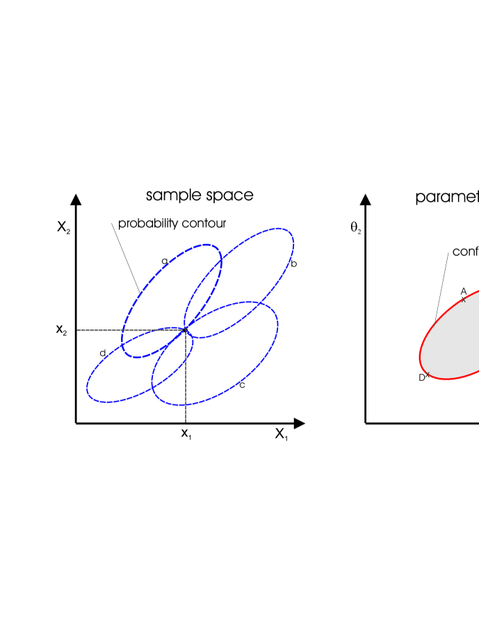
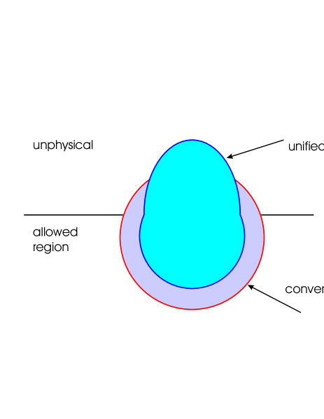
We illustrate the concept of CCL for a measurement (statistic) consisting of a two-dimensional observation ($x_{1},x_{2}$) and a two dimensional parameter space (see Fig. 1). In a first step we associate to each point $\theta_{1},\theta_{2}$ in the parameter space a closed probability contour in the sample space containing a measurement with probability $\alpha$. For example, the probability contour labeled $a$ in the sample space corresponds to the parameter values of point $A$ in the parameter space. The curve (confidence contour) connecting all points in the parameter space with probability contours in the sample space passing through the actual measurement $x_{1},x_{2}$ encloses the confidence region of confidence level $\alpha$.

Figure 1 demonstrates some of the requirements necessary for the construction of an exact confidence region: 1. The sample space must be continuous. (Discrete distributions and thus all digital measurements and in principle also Poisson processes are excluded.) 2. The probability contours should enclose a simply connected region. 3. The parameter space has to be continuous.

The restriction (1) usually is overcome by relaxing the requirement of exact coverage and by requiring minimum overcoverage. This is not an elegant solution.

There is considerable freedom in the choice of the probability contours but to insure coverage they have to be defined independently of the result of the experiment. Usually, contours are locations of constant probability density. In one dimension also central intervals and intervals leading to minimum sized confidence intervals are popular. Clearly, there is a lack of standardization. The unified approach [4] defines the probability regions through the likelihood ratio.

1.2 Likelihood limits and Bayesian conventions

Likelihood intervals enclose a region where the likelihood function decreases by a fixed ratio, equal to $\sqrt{e}$ for one standard deviation and $e^{2}$ for two standard deviations etc..

Figure 2: Likelihood limits (left) and Bayesian limits (right).

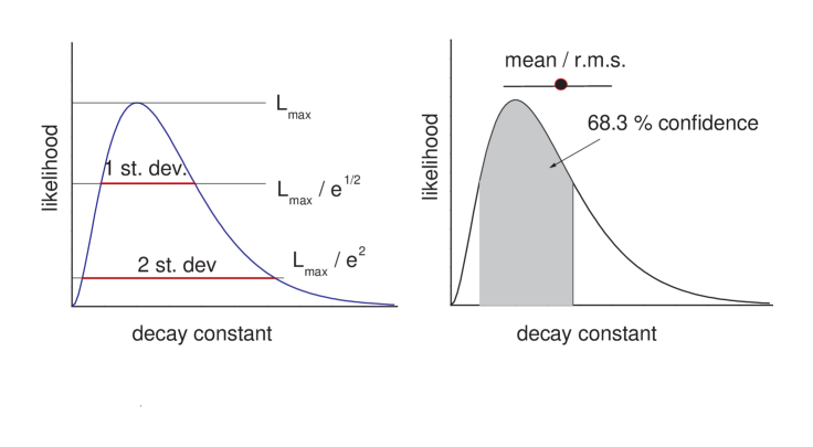
Bayesians integrate the normalized likelihood function and form either probability regions or moments to define the limits. I will discuss only uniform prior densities. This does not restrict the freedom of the scientist because there is the equivalent possibility to choose the parameter. For example an analysis using the mean life parameter with the prior $1/\tau^{2}$ is equivalent to an analysis of the decay constant $\gamma$ with uniform prior.

1.3 The likelihood principle

Assume we have two hypothesis characterized by the parameters $\theta_{1}$ and $\theta_{2}$. For a measurement $x_{1}$ the relative support to the two hypothesis is given by the likelihood ratio

$$R(x_{1}|\theta_{1},\theta_{2})=\frac{P(x_{1}|\theta_{1})}{P(x_{1}|\theta_{2})}$$

Another measurement $x_{2}$ is equivalent to $x_{1}$ if the likelihood ratios are the same:

$$\frac{P(x_{1}|\theta_{1})}{P(x_{1}|\theta_{2})}=\frac{P(x_{2}|\theta_{1})}{P(x_{2}|\theta_{2})}$$

When we have more than two hypothesis we require that equivalent date provide the same likelihood ratio for all combinations of parameters. Consequently, for a pdf depending on a continuous parameter $\theta,$ we have to require that the likelihood functions for the two measurements are proportional to each other. These considerations correspond to the Likelihood Principle (LP): The likelihood function contains the full information relative to the parameter. Inference should be based on the likelihood function only. The LP is due to Fisher, Birnbaum and others. Proofs and discussions can be found in Refs. [5, 6, 2].

Methods that provide different results for measurement that have proportional likelihood functions are inconsistent.

2 Examples

2.1 Example 1a: Gaussian with physical boundary

Figure 3: Gaussian errors near physical boundary (c: classical, cu: unified, l: likelihood, b: Bayesian). Left: 68.3% errors, right:90% upper limits.

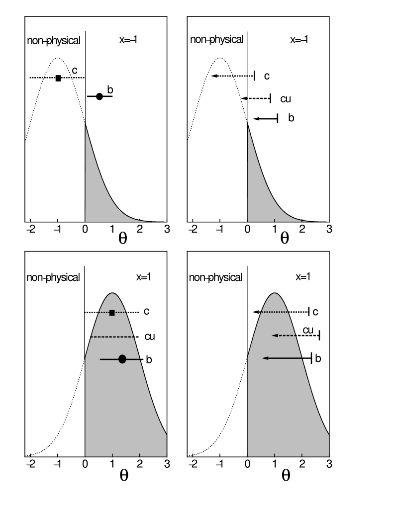
A physical quantity like the mass of a particle with a resolution following normal distributions is constrained to positive values. Fig. 3 shows typical central confidence bounds which extend into the unphysical region. In extreme cases a measurement may produce a 90 % confidence interval which does not cover positive values at all. The unified approach and the Bayesian method avoid unphysical confidence limits.

Figure 4: Disconected probability intervals in the unified approach. Gaussians (top) and Breit-Wigner (bottom).

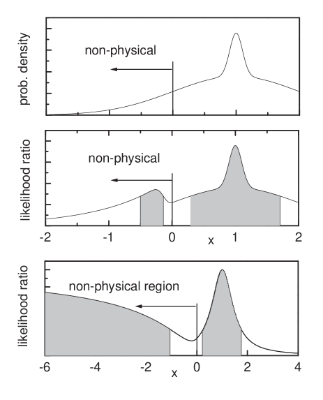
2.2 Example 1b: Superposition of Gaussians in the unified approach

The prescription for the construction of the probability intervals according to the likelihood ratio ordering leads to disconnected interval regions when the pdf has tails and cannot produce confidence intervals. This is shown in Fig. 4 top.

2.3 Example 1c: Breit-Wigner distribution

The same difficulty arises for the Breit-Wigner distribution (see Fig. 4 bottom).

The problem is absent if the pdf $f$ fulfills the condition $d^{2}\ln f/dx^{2}\geq 0$. This condition restricts the application of the unified approach to pdfs similar to Gaussians.

2.4 Example 2: Gaussian in two dimension and physical boundary

Let us assume that we have a Gaussian resolution in $x,y$ and a physical boundary in $y$ (Fig. 5). The probability contours are deformed in the unified approach as indicated in the sketch. As a consequence the error in $x$ shrinks due to a boundary in $y$ even though the two parameters are independent. One has to be careful in the interpretation of two-dimensional confidence limits as they occur for example in neutrino oscillation experiments.

Figure 5: Probabilty contours (schematic) for a two-dimensional Gaussian near a boundary in the unified approach.

2.5 Example 3: Slope of a linear distribution

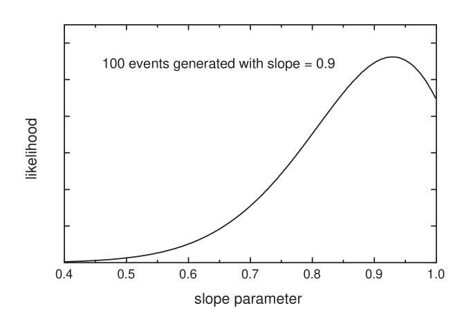
This is a frequent distribution in particle physics. A linear distribution is always restricted in the sample and the parameter space to avoid negative probabilities. We choose

$$f(x|\theta)=\frac{1}{2}(1+\theta x);\hskip 28.45274pt-1\leq\theta,x\leq 1$$

as is realized in many asymmetry distributions. For a sample of 100 events following the distribution of Equ. 2.4, a likelihood analysis gives a best value for the slope parameter of $\hat{\theta}=0.92$ (see Figure 6). There is no simple statistic allowing to compute central classical $62.8\%$ confidence limits because the parameter is undefined outside the interval [1,1]. Contrary to the conventional classical approach, the unified approach is able to handle the problem by working in the full sample space (hundred dimensional in our case) This requires a considerable computing effort.

Likelihood limits are possible - the upper limit would coincide with the boundary - but not well suited to measure the precision.

Figure 6: Likelihood for a slope parameter.

2.6 Example 4: Digital measurements

A particle track is passing at the unknown position $\mu$ through a proportional wire chamber. The measured coordinate $x$ is set equal to the wire location $x_{w}$. The probability density for a measurement $x$

$$f(x,\mu)=\delta(x-x_{w})$$

is independent of the true location $\mu$. Thus it is impossible to define a sensible classical confidence or likelihood interval, except a trivial one with full overcoverage. This difficulty is common to all digital measurements because they violate condition 1 of section 2.1. Thus a large class of measurements is not handled in classical statistics. A Bayesian treatment with uniform prior is the common solution. It provides the r.m.s. error $pitch/\sqrt{12}$.

2.7 Example 5: Gaussian with two physical boundaries

Figure 7: Two-sided physical boundary. Classical error bounds cover the full physical region.

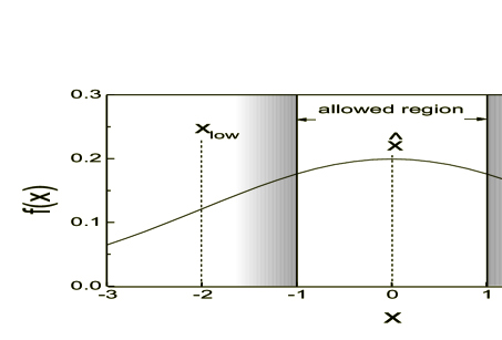
A particle passes through a small scintillator and another position sensitive detector with Gaussian resolution. Both boundaries of the classical error interval are in the region forbidden by the scintillator signal. (see Fig. 7) The classical error is twice as large as the r.m.s. width. It is meaningless. The unified classical and the likelihood limits contain the full physical region and thus are useless. Again only the Bayesian method gives reasonable results.

2.8 Example 6: Gaussian with variable width

A theory, depending on the unknown parameter $\theta$ predicts the Gaussian probability density

$$f(t)=\frac{25}{\sqrt{2\pi}\theta{}^{2}}\exp\left(-\frac{625(t-\theta)^{2}}{2\theta^{4}}\right)$$

for the time $t$ of an earthquake. The classical confidence interval for a measurement at $t=10$ h is $7.66<t_{3}<\infty$. It is shown together with the likelihood function in Fig. 8. When we look at the two distinct parameter values, predicting the time of an earthquake

Figure 8: Predictions from two discrete hypothesis H₁, H₂ and measurement (a) and log-likelihood for parametrization of the two hypothesis (b). The likelihood ratio strongly favors H₁which is excluded by the classical confidence limits.

$H_{1}$:	$t_{1}=(7.50\pm 2.25)$ h
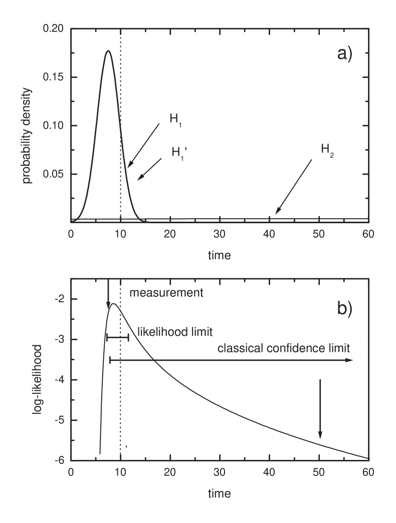
$H_{2}$:	$t_{2}=(50\pm 100)$ h

we realize that the first is excluded by the classical bounds, the second by the likelihood limits. The Fig. 8b shows the two probability densities together with the measurement. Clearly, we would rather accept $H_{1}$. This choice is also supported by the likelihood ratio which is in favor of H₁ by a factor 26. Thus the likelihood limits are intuitively more acceptable than the classical ones.

The preceding example shows that the concept of classical confidence limits for continuous parameters is not compatible with methods based on the likelihood values. We may construct a transition from the discrete case to the continuous one by adding more and more hypothesis but a transition from likelihood based methods to CCL is impossible. The two classical approaches CCL and Neyman-Pearson test lack a common bases.

2.9 Example 6b: Number of neutrinos

This example was presented by Cousins [7]: MarkII had measured the number of neutrinos to be $2.8\pm 0.6$ and deduced a 95% confidence upper limit of 3.9 excluding 4 neutrino generations. The likelihood ratio of 7.0 produces a much weaker exclusion of the discrete hypothesis.

2.10 Example 7: Stopping rule

A rate measurement may be stopped for reasons like: i) There are enough events. ii) For a long time no event has been observed. iii) A “golden” event was recorded.

Figure 9: A sequential stopping rule does not introduce a bias.

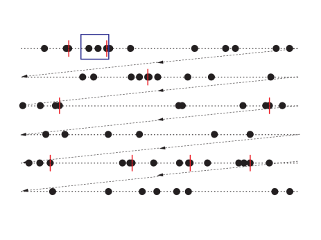
These actions do not introduce a bias as has been first realized by Barnard and co-workers [8]. The reason is that the likelihood function is independent of the stopping rule. This may be visualized by an infinitely long measurement which is cut in pieces each corresponding to a experiment stopped by the same rule. The individual experiment cannot be biased since the full chain is unbiased. This is illustrated in Fig. 9 where the experiments are stopped whenever 3 events are recorded in a short time interval.

Figure 10: Stopping after a fixed time or when a fixed number of events has been observed (same likelihood) gives different results in classical statistics.

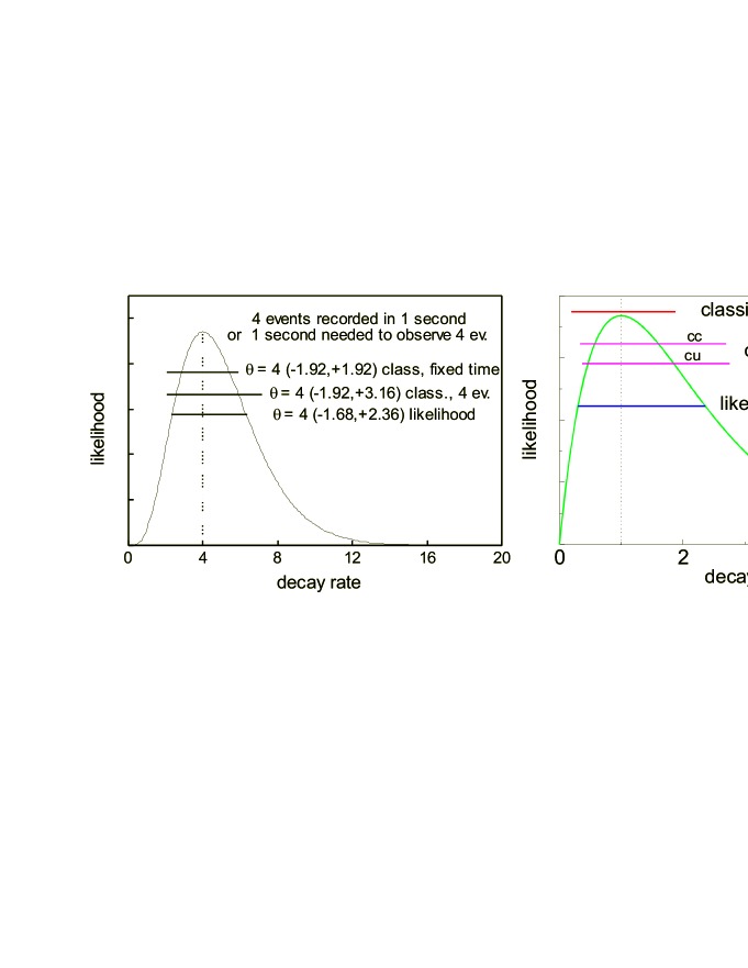
The Figure 10 shows the likelihood function for an experiment where 4 events are observed in a time interval of one second. The classical results depend on the stopping condition: a) the time interval had been fixed, b) the experiment was stopped after the forth event. The likelihood principle states that the two data sets are equivalent. Thus the classical limits are inconsistent.

The differences become even larger when we take the example of 1 event recorded in 1 second (see Fig. 10 right). The likelihood functions given by the lifetime distribution and the Poisson distribution, respectively are proportional to each other

$$f(t|\lambda) =\lambda e^{-\lambda t}$$

$$P(1|\lambda) =\frac{e^{-\lambda}\lambda^{1}}{1!}$$

2.11 Example 8: Poisson signal with background

In a garden there are apple and pear trees. Usually during night some pears fall from the trees. One morning looking from his window, the proprietor who is interested in apples find that no fruit is lying in the grass. Since it is still quite dark he is unable to distinguish apples from pears. He concludes that the average rate of falling apples per night is less the 2.3 with 90% confidence level. His wife who is a classical statistician tells him that his rate limit is too high because he has forgotten to subtract the expected pears background. He argues, “there are no pears”, but she insists and explains him that if he ignores the pears that could have been there but weren’t, he would violate the coverage requirement. In the meantime it has become bright outside and pears and apples - which both are not there - are now distinguishable. Even though the evidence has not changed, the classical limit has.

The 90% confidence limits for zero events observed and background expectation $b=0$ is $\mu=2.3$. For $b=2$ it is $\mu^{\prime}=0.3$ much lower. CCL are different for two experiments with exactly the same experimental evidence relative to the signal (no signal event seen). This situation is absolutely intolerable. Feldman and Cousins consider this kind of objections as “based on a misplaced Bayesian interpretation of classical intervals” [4]. It is hard to detect a Bayesian origin in a generally accepted principle in science, namely, two measurements containing the same information should give identical results. The critics here is not that CCLs are inherently wrong but that their application to the computation of upper limits when background is expected does not make sense, i.e. these limits do not measure the precision of the experiment.

The effect is less dramatic but also present in the unified approach: An experiment finding no event n=0 with background expectation b=3 produces a 90% confidence limit 1.08 for the signal (see Table 2.1). Then the flux is doubled and the background is eliminated. The limit becomes 2.44/2=1.22, worse than before. This problem is absent in the versions proposed by Roe and Woodroofe [9] and also in that of Punzi [10]. These methods are however restricted to the Poisson case.

	n=0, b=0	n=0, b=1	n=0, b=2	n=0, b=3	n=2, b=2
standard classical	2.30	1.30	0.30	-0.70	3.32
unified classical	2.44	1.61	1.26	1.08	3.91
uniform Bayesian	2.30	2.30	2.30	2.30	3.88

Table 1: Poisson limits in classical and Bayesian approaches

To avoid the unacceptable situation, I have proposed a modified frequentist approach to the calculation of the Poissonian limits including the information of the limited number of background events [11]. There the confidence level is normalized to the probability to observe $0\leq n_{b}\leq n$ background events as known from the measurement.

$$1-\alpha=\frac{\sum_{i=0}^{n}P(i|\mu+b)}{\sum_{i=0}^{n}P(i|b)}$$

The resulting limits respect the likelihood principle (see below) and thus are consistent. They coincide with those of the uniform Bayesian method and provide a frequentist interpretation of the Bayesian limits. However, as has been pointed out by Highland [12], the limits do not have minimum overcoverage as required by the strict application of the Neyman construction. This is correct [13] but in my paper no claim relative coverage had been made. The method has been applied to the a Higgs search [14].

Figure 11: Coverage in the unified classical and the Bayesian approach (dotted) and interval lengths (bottom).

Often the background expectation is not known precisely since it is estimated from side bands or from other measurements with limited statistics. So far, there is no classical recipe which allows to incorporate an uncertainty of the background estimate.

Likelihood limits also give a sensible description of the data. Whether likelihood limits or Bayesian limits obtained from the integration are more sensible depends on the shape of the likelihood function. Ideally both limits should be given.

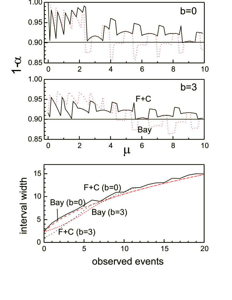
Fig. 11 compares the coverage of the unified classical and the Bayesian limits. At small signals both overcover strongly. For large signals the Bayesian method slightly undercovers and oscillates around the nominal value.

2.12 Example 9: Combining lifetime measurements

Two events are observed from an exponential decay with true mean life $\tau_{0}=1/\gamma_{0}$. The maximum likelihood estimate is used either for $\tau$ or $\gamma$. We assume that an infinite number of identical experiments is performed and that the results are combined. In Table 2.2 we summarize the results of different averaging procedures. There is no prescription for averaging classical intervals. The unified methods have to explain how they intend to combine their measurements. To compute the classical result given in the table, the maximum likelihood estimate and central intervals were used.

method	$<\tau/\tau_{0}>$	$<\gamma/\gamma_{0}>$
adding log likelihood functions	$1$	$1$
classical, weight: $\sigma^{-2}$	$0.0$	$0.67$
likelihood, weight: PDG	$0.26$	$0.80$
Bayesian mean, uniform prior, weight: $\sigma^{-2}$	$\infty$	$1$

Table 2: Average of an infinite number of equivalent lifetime measurements using different weighting procedures

Figure 12: Log-likelihood function of the mean life and the decay rate.

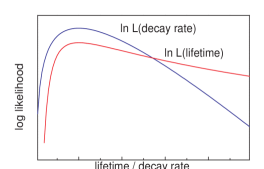
In this special example a consistent result is obtained in the Bayesian method with uniform prior for the decay constant. It shows also how critical the choice of the parameter is in the Bayesian approach. It is also clear that an educated choice is also important for the pragmatic procedures. It is obvious that the decay constant is the better parameter (see also Fig. 12). Methods approximating the likelihood function provide reasonable results unless the likelihood function is very asymmetric. The weighting procedure of the PDG applied to the likelihood errors gives reasonable results. As is well known, adding the log-likelihood functions always produces a correct result.

3 Conclusions

3.1 Conventional classical method

The conventional classical schemes suffer from the following problems:

• There are inconsistencies ( Poisson limits, stopping rule, discrete vs. continuous parameters).

• There is a lack of precision (unphysical limits).

• They have a restricted range of application (problems with digital measurements, discrete parameters).

• They are not invariant against sample variable transformations (except central intervals in one dimension).

• They are subjective (coverage requires pre-experimental fixing of cuts and decision to publish).

• There are unsolved problems. (It is not clear how to combine measurements. The inclusion of background errors in Poisson processes is not possible.)

• There is no obvious treatment of nuisance parameters.

• Systematic errors cannot be included.

3.2 Unified approach

Compared to the conventional method there are improvements:

• The inconsistencies in Poisson processes are weaker ( and absent in the version of Roe and Woodroofe)

• Non-physical limits are avoided.

• It is invariant with respect to variable and parameter transformations.

However most problems remain (inconsistencies, lack of precision, background uncertainty in Poisson limits), and:

• It is restricted to specific pdfs (Gaussian like).

• It is complicated and requires considerable computing efforts.

• The combination of measurements is even more unclear.

• Artificial error correlations are introduced near boundaries.

• The proposed treatment [16] of nuisance parameters (use best estimate may lead to undercoverage.

3.3 Likelihood limits

Likelihood limits have attractive properties

• They are consistent.

• They provide optimum precision.

• They are invariant against variable and parameter transformations.

• They provide a coherent transition to discrete hypothesis (likelihood ratio)

• Measurements can easily be combined

There are also restrictions in the application:

• Digital measurements and uniform distributions cannot be handled.

3.4 Bayesian limits

The Bayesian philosophy is very general and flexible:

• All problems can be treated. (Nuisance parameters, digital measurements, unphysical boundaries etc.)

but:

• They depend on the parameter choice.

4 Proposed conventions

The conventions proposed here represent by no means the only reasonable prescription.

Since the complete information is contained in the likelihood function, classical approaches are not considered. (They cannot be computed from the likelihood function alone.) An even stronger reason for there exclusion are the obvious inconsistencies of this method.

The main objection against Bayesian methods is their dependence on the selected parameter. I find it rather natural to choose a sensible parameter space. For some application like pattern recognition - which, by the way, cannot be done with classical statistics - it is absolutely necessary.

The proposed conventions are:

1. Whenever possible the full likelihood function should be published. It contains the experimental information and permits to combine the results of different experiments in an optimum way. This is especially important when the likelihood is strongly non-Gaussian (strongly asymmetric, cut by external bounds, has several maxima etc.).

2. Data are combined by adding the log-likelihoods. When not known, parametrizations are used to approximate it.

3. If the likelihood is smooth and has a single maximum the likelihood limits should be given to define the error interval. These limits are invariant under parameter transformation. For the measurement of the parameter the value maximizing the likelihood function is chosen. No correction for biased likelihood estimators is applied. The errors usually are asymmetric. These limits can also be interpreted as Bayesian one standard deviation errors for the specific choice of the parameter variable where the likelihood of the parameter has a Gaussian shape.

4. Nuisance parameters are eliminated by integrating them out using an uniform prior. A correlation coefficient should be computed.

5. For digital measurements the Bayesian mean and r.m.s. should be used.

6. In cases where the likelihood function is restricted by physical or mathematical bounds and where there are no good reasons to reject an uniform prior the measurement and its errors defined as the mean and r.m.s. should be computed in the Bayesian way.

7. Upper and lower limits are computed from the tails of the Bayesian probability distributions. (In some cases likelihood limits may be more informative. [15])

8. Non-uniform prior densities should not be used.

9. It is the scientist’s choice whether to present an error interval or an upper limit.

10. In any case the applied procedure has to be documented.

These recipes correspond more or less to our every day practice. An exception are Poisson limits where for strange reasons the coverage principle - though only approximately realized - has gained preference in neutrino experiments.

Acknowledgement

I would like to thank Fred James, Louis Lyons and Yves Perrin for having organized this interesting workshop which - for the first time - offered the possibility to high energy physicists to expose and discuss their problems and solutions to statistical problems.

References

- [1] I. Narsky, Estimation of Upper Limits Using a Poisson Statistic, hep-ex/9904025 (1999)
- [2] A. W. F. Edwards, Likelihood, The John Hopkins University Press, Baltimore (1992)
- [3] G. Zech, Objections to the unified approach to the computation of classical confidence limits, physics/9809035
- [4] G. J. Feldman, R. D. Cousins, Unified approach to the classical statistical analysis of small signals. Phys. Rev. D 57 (1998) 1873.
- [5] D. Basu, Statistical Information and Likelihood, Lecture Notes in Statistics, ed. J.K. Ghosh, Springer-Verlag NY (1988)
- [6] J. O. Berger and R. L. Wolpert, The likelihood Principle, Lecture Notes of Inst. of Math. Stat., Hayward, Ca, (ed. S. S. Gupta) (1984)
- [7] R. D. Cousins, Why Isn’t Every Physicist a Bayesian? Am J. Phys. 63 (1995) 398
- [8] G. A. Barnard, G. M. Jenkins and C. B. Winstein, Likelihood inference and time series, J. Roy. Statist. Soc. A 125 (1962)
- [9] B. P. Roe and M. B. Woodroofe, Improved probability method for estimating signal in the presence of background, Phys. Rev. D 60, 053009 (1999)
- [10] G. Punzi, A stronger classical definition of confidence limits, hep-ex/9912048 (1999)
- [11] G. Zech, Upper limits in experiments with background or measurement errors, Nucl. Instr. and Meth. A277 (1989) 608-610
- [12] V. L. Highland, Comments on “Upper limits in experiments with background or measurement errors”, Nucl. Instr. and Meth. A 398 (1997) 429
- [13] G. Zech, Reply to ’Comments on “Upper limits in experiments with background or measurement errors” ’, Nucl. Instr. and Meth. A398 (1997) 431-433
- [14] A. L. Read, Optimal statistical analysis of search results based on the likelihood ratio and its application to the search for the MSM Higgs boson at = 161 and 172 GeV, DELPHI 97-158 PHYS 737 (1997)
- [15] G. D’Agostini, Contribution to this workshop
- [16] R. D. Cousins, Contribution to this workshop