Abstract

Hadron energy reconstruction for the Atlas barrel prototype combined calorimeter, consisting of the lead-liquid argon electromagnetic part and the iron-scintillator hadronic part, in the framework of the non-parametrical method has been fulfilled. This method uses only the known $e/h$ ratios and the electron calibration constants and does not require the determination of any parameters by a minimization technique. The obtained reconstruction of the mean values of energies is within $\pm 1\%$ and the fractional energy resolution is $[(58\pm 3)\%\sqrt{GeV}/\sqrt{E}+(2.5\pm 0.3)\%]\oplus(1.7\pm 0.2)\ GeV/E$. The obtained value of the $e/h$ ratio for electromagnetic compartment of the combined calorimeter is $1.74\pm 0.04$ and agrees with the prediction that $e/h>1.7$ for this electromagnetic calorimeter. The results of the study of the longitudinal hadronic shower development are presented. The data have been taken in the H8 beam line of the CERN SPS using pions of 10 – 300 GeV.
Keywords: Calorimetry; Computer data analysis.

1 Introduction

The key question of calorimetry generally and hadronic calorimetry in particular is the energy reconstruction. This question is especially important when a hadronic calorimeter have a complex structure being a combined calorimeter. Such is the combined calorimeter with the electromagnetic and hadronic compartments of the ATLAS detector [1, 2, 3]. In this paper we describe the non-parametrical method of the energy reconstruction for a combined calorimeter, which called the $e/h$ method, and demonstrate its performance on the basis of the test beam data of the ATLAS combined prototype calorimeter. For the energy reconstruction and description of the longitudinal development of a hadronic shower it is necessary to know the $e/h$ ratios, the degree of non-compensation, of these calorimeters. As to the ATLAS Tile barrel calorimeter there is the detailed information about the $e/h$ ratio presented in [2, 4, 5, 6, 7]. But as to the liquid argon electromagnetic calorimeter such information is practically absent. The aim of the present work is also to develop the method and to determine the value of the $e/h$ ratio of the electromagnetic compartment.

One of the important questions of hadron calorimetry is the question of the longitudinal development of hadronic showers. This question is especially important for a combined calorimeter. This work is also devoted to the study of the longitudinal hadronic shower development in the ATLAS barrel combined prototype calorimeter.

This work has been performed on the basis of the 1996 combined test beam data [8, 9]. The data have been taken in the H8 beam line of the CERN SPS using pions of 10, 20, 40, 50, 80, 100, 150 and 300 GeV.

2 Combined Calorimeter

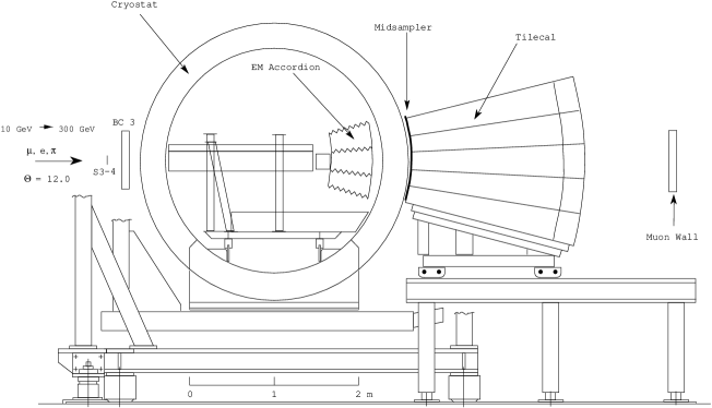
Figure 1: Test beam setup for the combined LAr and Tile calorimeters run.

The combined calorimeter prototype setup has been made consisting of the LAr electromagnetic calorimeter prototype inside the cryostat and downstream the Tile calorimeter prototype as shown in Fig. 1. The two calorimeters have been placed with their central axes at an angle to the beam of $12^{\circ}$. At this angle the two calorimeters have an active thickness of 10.3 $\lambda_{I}$. Beam quality and geometry were monitored with a set of beam wire chambers BC1, BC2, BC3 and trigger hodoscopes placed upstream of the LAr cryostat. To detect punchthrough particles and to measure the effect of longitudinal leakage a “muon wall” consisting of 10 scintillator counters (each 2 cm thick) was located behind the calorimeters at a distance of about 1 metre.

2.1 Electromagnetic Calorimeter

The electromagnetic LAr calorimeter prototype consists of a stack of three azimuthal modules, each one spanning $9^{\circ}$ in azimuth and extending over 2 m along the Z direction. The calorimeter structure is defined by 2.2 mm thick steel-plated lead absorbers folded to an accordion shape and separated by 3.8 mm gaps filled with liquid argon. The signals are collected by Kapton electrodes located in the gaps. The calorimeter extends from an inner radius of 131.5 cm to an outer radius of 182.6 cm, representing (at $\eta=0$) a total of 25 radiation lengths ($X_{0}$), or 1.22 interaction lengths ($\lambda_{I}$) for protons. The calorimeter is longitudinally segmented into three compartments of $9\ X_{0}$, $9\ X_{0}$ and $7\ X_{0}$, respectively. More details about this prototype can be found in [1, 10].

The cryostat has a cylindrical form with 2 m internal diameter, filled with liquid argon, and is made out of a 8 mm thick inner stainless-steel vessel, isolated by 30 cm of low-density foam (Rohacell), itself protected by a 1.2 mm thick aluminum outer wall.

2.2 Hadronic Calorimeter

The hadronic Tile calorimeter is a sampling device using steel as the absorber and scintillating tiles as the active material [2]. The innovative feature of the design is the orientation of the tiles which are placed in planes perpendicular to the Z direction [11]. For a better sampling homogeneity the 3 mm thick scintillators are staggered in the radial direction. The tiles are separated along Z by 14 mm of steel, giving a steel/scintillator volume ratio of 4.7. Wavelength shifting fibres (WLS) running radially collect light from the tiles at both of their open edges. The hadron calorimeter prototype consists of an azimuthal stack of five modules. Each module covers $2\pi/64$ in azimuth and extends 1 m along the Z direction, such that the front face covers $100\times 20$ cm². The radial depth, from an inner radius of 200 cm to an outer radius of 380 cm, accounts for 8.9 $\lambda$ at $\eta=0$  (80.5 $X_{0}$). Read-out cells are defined by grouping together a bundle of fibres into one photomultiplier (PMT). Each of the 100 cells is read out by two PMTs and is fully projective in azimuth (with $\Delta\phi=2\pi/64\approx 0.1$), while the segmentation along the Z axis is made by grouping fibres into read-out cells spanning $\Delta Z=20$ cm ($\Delta\eta\approx 0.1$) and is therefore not projective. Each module is read out in four longitudinal segments (corresponding to about 1.5, 2, 2.5 and 3 $\lambda_{I}$ at $\eta=0$). More details of this prototype can be found in [1, 12, 13, 14, 15].

2.3 Data Selection

The data have been taken in the H8 beam line of the CERN SPS using pions of 10, 20, 40, 50, 80, 100, 150 and 300 GeV. We applied some similar to [8, 9] cuts to eliminate the non-single track pion events, the beam halo, the events with an interaction before the LAr calorimeter, the electron and muon events. The set of cuts is the following: the single-track pion events were selected by requiring the pulse height of the beam scintillation counters and the energy released in the presampler of the electromagnetic calorimeter to be compatible with that for a single particle; the beam halo events were removed with appropriate cuts on the horizontal and vertical positions of the incoming track impact point and the space angle with respect to the beam axis as measured with the beam chambers; a cut on the total energy rejects incoming muon.

3 $e/h$ Method of Energy Reconstruction

The response, $R$, of a calorimeter to a hadronic shower is the sum of the contributions from the electromagnetic, $E_{e}$, and hadronic, $E_{h}$, parts of the incident energy $E$ [16, 17]:

$$R=e\cdot E_{e}+h\cdot E_{h}=e\cdot E\cdot(f_{\pi^{0}}+(h/e)\cdot(1-f_{\pi^{0}}))\ ,$$ (1)

$$E=E_{e}+E_{h}\ ,$$ (2)

where $e$ ($h$) is the energy independent coefficient of transformation of the electromagnetic (pure hadronic, low-energy hadronic activity) energy to response, $f_{\pi^{0}}=E_{e}/E$ is the fraction of electromagnetic energy. From this

$$E=\Bigl{(}\frac{e}{\pi}\Bigr{)}\cdot\frac{R}{e}\ ,$$ (3)

and

$$\frac{e}{\pi}=\frac{e/h}{1+(e/h-1)f_{\pi^{0}}}\ .$$ (4)

For a combined calorimeter the incident energy deposits into the LAr compartment, $E_{LAr}$, the Tile calorimeter compartment, $E_{Tile}$, and into the passive material between the LAr and Tile calorimeters, $E_{dm}$,

$$E=E_{LAr}+E_{dm}+E_{Tile}\ .$$ (5)

Using the expressions (3) – (5) the following equation for the energy reconstruction has been derived:

$$E=\sum_{i}c_{i}\cdot\Bigl{(}\frac{e}{\pi}\Bigr{)}_{i}\cdot R_{i}=c_{LAr}\cdot\Bigl{(}\frac{e}{\pi}\Bigr{)}_{LAr}\cdot R_{LAr}+E_{dm}+c_{Tile}\cdot\Bigl{(}\frac{e}{\pi}\Bigr{)}_{Tile}\cdot R_{Tile}\ ,$$ (6)

where $i=LAr,\ dm,\ Tile$; $c_{i}=1/e_{i}$; $(e/\pi)_{i}$ are from equation (4) and

$$f_{\pi^{0},\ LAr}=k\cdot\ln{(E)}\ ,$$ (7)

$$f_{\pi^{0},\ Tile}=k\cdot\ln{(E_{Tile})}\ ,$$ (8)

where $E_{Tile}=c_{Tile}\cdot(e/\pi)_{Tile}\cdot R_{Tile}$ and $k=0.11$. Note, that for $\approx 70\%$ of events an energy in Tile calorimeter is approximately equal to beam energy because a hadronic shower began in the hadron calorimeter.

The term, which accounts for the energy loss in the dead material between the LAr and Tile calorimeters, $E_{dm}$, is taken to be proportional to the geometrical mean of the energy released in the third depth of the electromagnetic compartment ($E_{LAr,\ 3}=c_{LAr}\cdot(e/\pi)_{LAr}\cdot R_{LAr,\ 3}$) and the first depth of the hadronic compartment ($E_{Tile,\ 1}=c_{Tile}\cdot(e/\pi)_{Tile}\cdot R_{Tile,\ 1}$)

$$E_{dm}=c_{dm}\cdot\sqrt{E_{LAr,3}\cdot E_{Tile,1}}$$ (9)

similar to [8, 18]. The validity of this approximation has been tested by the Monte Carlo simulation and by the study of the correlation between the energy released in the midsampler and the cryostat energy deposition [9, 19, 20]. The value of $c_{dm}=0.31$ obtained on the basis of the results of the Monte Carlo simulation is used.

In order to use the equation (6) it is necessary to know the values of the following constants: $c_{LAr}$, $c_{dm}$, $c_{Tile}$, $(e/h)_{LAr}$, $(e/h)_{Tile}$, some of which are $c_{LAr}=1/e_{LAr}=1.1$ [8, 9], $(e/h)_{Tile}=1.3\pm 0.03$ [6]. The determination of the other constants ($c_{dm}$, $c_{Tile}$, $(e/h)_{LAr}$) is given below.

3.1 $c_{Tile}$ Constant

For the determining of the $c_{Tile}$ constant the following procedure was applied. We selected the events which start to shower only in the hadronic calorimeter. To select these events the energies deposited in each sampling of the LAr calorimeter and in the midsampler are required to be compatible with that of a single minimum ionization particle.

The following expression for the normalized hadronic response have been used [17]:

$$\frac{R_{Tile}^{c}}{E_{beam}}=\frac{1+((e/h)_{Tile}-1)\cdot f_{\pi^{0},\ Tile}}{c_{Tile}\cdot(e/h)_{Tile}}\ ,$$ (10)

where

$$R_{Tile}^{c}=R_{Tile}+\frac{c_{LAr}}{c_{Tile}}\cdot R_{LAr}$$ (11)

is the Tile calorimeter response corrected on the energy loss in the LAr calorimeter, $f_{\pi^{0},Tile}$ is determined by the formula (8). The value of $c_{Tile}$ obtained by fitting is equal to $0.145\pm 0.002$.

3.2 $e/h$ ratio of Electromagnetic Compartment

Using the expression (6) the value of the $(e/\pi)_{LAr}$ ratio can be obtained

$$\Bigl{(}\frac{e}{\pi}\Bigr{)}_{LAr}=\frac{E_{beam}-E_{dm}-E_{Tile}}{c_{LAr}\cdot R_{LAr}}\ .$$ (12)

The $(e/h)_{LAr}$ ratio and the function $f_{\pi^{0},LAr}$ (7) can be inferred from the energy dependent $(e/\pi)_{LAr}$ ratios.

For this case we select the events with the well developed hadronic showers in the electromagnetic calorimeter. Than mean that energy depositions were required to be more than 10% of the beam energy in the electromagnetic calorimeter and less than 70% in the hadronic calorimeter.

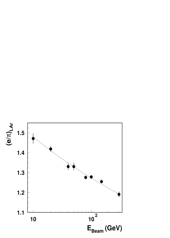
Figure 3: The mean value of the $(e/\pi)_{LAr}$ ratio as a function of the beam energy. The curve is the result of a fit of equation (4).

Fig. 2 shows the distributions of the $(e/\pi)_{LAr}$ ratio derived by formula (12) for different energies. The mean values of these distributions are shown in Fig. 3 as a function of the beam energy. The fit of this distribution by the expression (4) for LAr calorimeter yields $(e/h)_{LAr}=1.74\pm 0.04$ and $k=0.108\pm 0.004$. The quoted errors are the statistical ones obtained from the fit. The systematic error on the $(e/h)_{LAr}$ ratio, which is a consequence of the uncertainties in the input constants used in the equation (12), is estimated to be $\pm 0.04$.

Wigmans showed [21] that the $e/h$ ratio for non-uranium calorimeters with high-Z absorber material is satisfactorily described by the formula:

$$\frac{e}{h}=\frac{e/mip}{0.41+0.12\cdot n/mip}$$ (13)

in which $e/mip$ and $n/mip$ represent the calorimeter response to e.m. showers and to MeV-type neutrons, respectively. These responses are normalized to the one for minimum ionizing particles. The Monte Carlo calculated $e/mip$ and $n/mip$ values for the R&D3 Pb-LAr electromagnetic calorimeter are $e/mip=0.78$ [21] and $n/mip<0.5$ [21] leading to $(e/h)_{LAr}>1.66$. Our measured value of the $(e/h)_{LAr}$ ratio agrees with this prediction.

3.3 Iteration Procedure

For the energy reconstruction by the formula (6) it is necessary to know the $(e/\pi)_{Tile}$ ratio and the reconstructed energy itself. Therefore, the iteration procedure has been developed. Two iteration cycles were made: the first one is devoted to the determination of the $(e/\pi)_{Tile}$ ratio and the second one is the energy reconstruction itself.

The expression (4) for the $(e/\pi)_{Tile}$ ratio can be written as

$$\Bigl{(}\frac{e}{\pi}\Bigr{)}_{Tile}=\frac{(e/h)_{Tile}}{1+((e/h)_{Tile}-1)\cdot k\cdot\ln{(c_{Tile}\cdot(e/\pi)_{Tile}\cdot R_{Tile})}}\ .$$ (14)

As the first approximation, the value of $(e/\pi)_{Tile}$ is calculated using the equation (14) where in the right side of this equation we used $(e/\pi)_{Tile}=1.13$ corresponding to $f_{\pi^{0},Tile}=0.5=0.11\ln{(100\ GeV)}$. The iteration process is stopped when the convergence criterion $\mid(e/\pi)_{Tile}^{\nu+1}-(e/\pi)_{Tile}^{\nu}\mid/(e/\pi)_{Tile}^{\nu}<\epsilon$, where ($\nu=0,\ 1,\ldots$), is satisfied.

As the first approximation in the iteration cycle for the energy reconstruction, the value of $E$ is calculated using the equation (6) with the $(e/\pi)_{Tile}$ ratio obtained in the first iteration cycle and $(e/\pi)_{LAr}$ from equation (4) where in the right side of this equation we used $(e/\pi)_{LAr}=1.27$ corresponding to $f_{\pi^{0},LAr}=0.5=0.11\ln{(100\ GeV)}$. The convergence criterion is $\mid E^{\nu+1}-E^{\nu}\mid/E^{\nu}<\epsilon$.

For both these case the iteration values are under the logarithmic function that mean that iteration procedure will be very fast.

The average numbers of iterations $<N_{it}>$ for the various beam energies needed to receive the given value of accuracy $\epsilon$ have been investigated. It turned out, it is sufficiently only the first approximation for achievement, on average, of convergence with an accuracy of $\epsilon=1\%$ for energies 80 – 150 $GeV$ and it is necessary to perform only one iteration for the energies at 10 – 50 $GeV$ and 300 $GeV$.

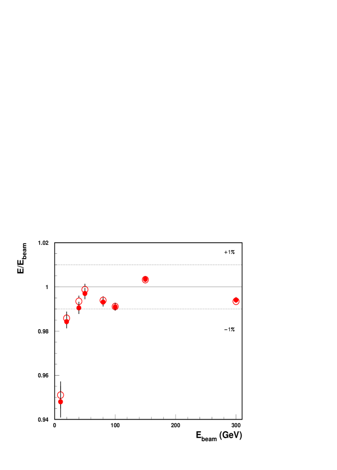
Figure 4: Energy linearity as a function of the beam energy for the $e/h$ method obtained using the iteration procedure with $\epsilon=0.1\%$ (black circles) and the first approximation (open circles).

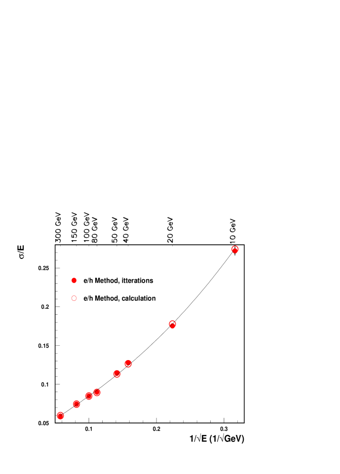
Figure 5: The fractional energy resolutions obtained with the $e/h$ method (black circles), and the first approximation (open circles).

We specially investigated the accuracy of the first approximation of energy. Fig. 4 shows the comparison between the energy linearities, the mean values of $E/E_{beam}$, obtained using the iteration procedure with $\epsilon=0.1\%$ (black circles) and the first approximation of energy (open circles). Fig. 5 shows the comparison between the energy resolutions obtained using these two approaches. As can be seen, the compared values are consistent within errors.

The suggested algorithm of the energy reconstruction can be used for the fast energy reconstruction in the first level trigger.

3.4 Energy Spectra

Fig. 6 shows the pion energy spectra reconstructed with the $e/h$ method ($\epsilon=0.1\%$). The mean and $\sigma$ values of these distributions are extracted with Gaussian fits over $\pm 2\sigma$ range. The obtained mean values $E$, the energy resolutions $\sigma$, and the fractional energy resolutions $\sigma/E$ are listed in Table 1 for the various beam energies.

3.5 Energy Linearity

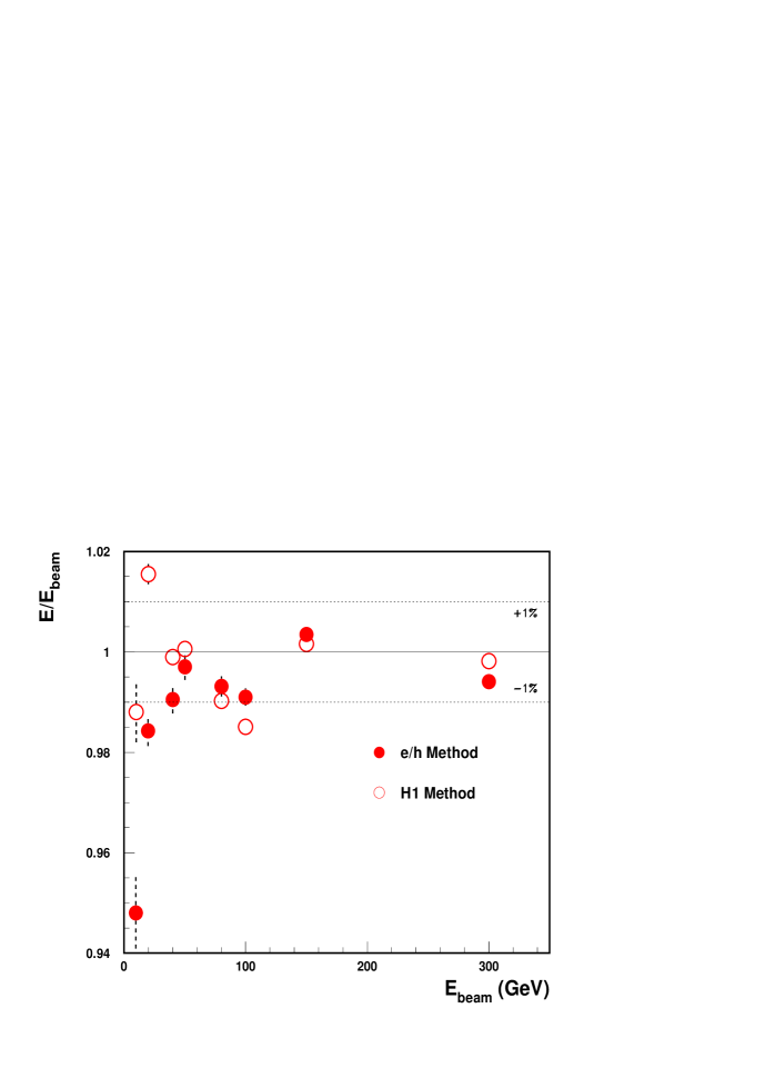
Figure 7: Energy linearity as a function of the beam energy for the $e/h$ method (black circles) and the cells weighting H1 method (open circles).

Fig. 7 demonstrates the correctness of the mean energy reconstruction. The mean value of $E/E_{beam}$ is equal to $(99.5\pm 0.3)\%$ and the spread is $\pm 1\%$ except for the point at 10 $GeV$. But, as noted in [8], at this point the result is strongly dependent on the effective capability to remove events with interactions in the dead material upstream and to deconvolve the real pion contribution from the muon contamination. Fig. 7 also shows the comparison of the linearity, $E/E_{beam}$, as a function of the beam energy for the $e/h$ method and for the cells weighting method [8]. As can be seen, the comparable quality of the linearity is observed for these two methods.

3.6 Energy Resolutions

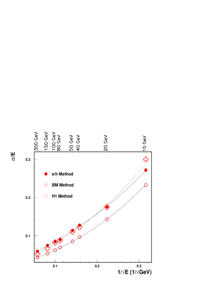
Figure 8: The energy resolutions obtained with the $e/h$ method (black circles), the benchmark method (crosses) and the cells weighting method (circles).

Fig. 8 shows the fractional energy resolutions ($\sigma/E$) as a function of $1/\sqrt{E_{beam}}$ obtained by three methods: the $e/h$ method (black circles), the benchmark method [8] (crosses), and the cells weighting method [8] (open circles). As can be seen, the energy resolutions for the $e/h$ method are comparable with the benchmark method and only of $30\%$ worse than for the cells weighting method. A fit to the data points gives the fractional energy resolution for the $e/h$ method obtained using the iteration procedure with $\epsilon=0.1\%$: $\sigma/E=[(58\pm 3)\%\sqrt{GeV}/\sqrt{E}+(2.5\pm 0.3)\%]\oplus(1.7\pm 0.2)\ GeV/E$, for the $e/h$ method using the first approximation: $\sigma/E=[(56\pm 3)\%\sqrt{GeV}/\sqrt{E}+(2.7\pm 0.3)\%]\oplus(1.8\pm 0.2)\ GeV/E$, for the benchmark method of $\sigma/E=[(60\pm 3)\%\sqrt{GeV}/\sqrt{E}+(1.8\pm 0.2)\%]\oplus(2.0\pm 0.1)\ GeV/E$, for the cells weighting method of $\sigma/E=[(42\pm 2)\%\sqrt{GeV}/\sqrt{E}+(1.8\pm 0.1)\%]\oplus(1.8\pm 0.1)\ GeV/E$, where the symbol $\oplus$ indicates a sum in quadrature. As can be seen, the sampling term is consistent within errors for the $e/h$ method and the benchmark method and is smaller by 1.5 times for the cells weighting method. The constant term is the same for the benchmark method and the cells weighting method and is larger by $(0.7\pm 0.3)\%$ for the $e/h$ method. The noise term of about $1.8\ GeV$ is the same for these three methods that reflects its origin as the electronic noise. As to the two approaches for the $e/h$ method, the fitted parameters coincide within errors.

4 Hadronic Shower Development

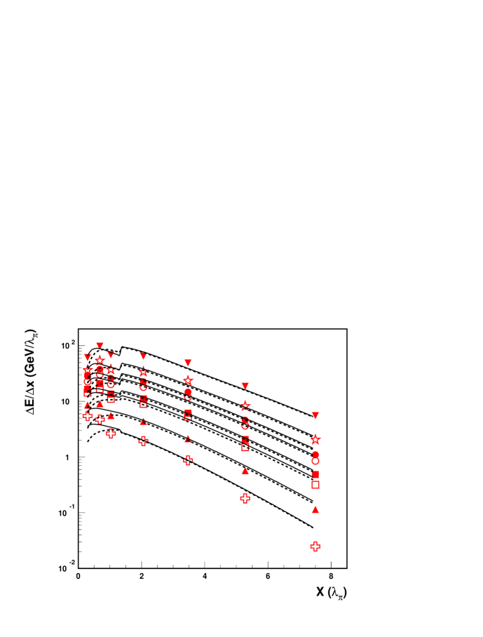
Figure 9: The experimental differential longitudinal energy depositions at 10 GeV (crosses), 20 GeV (black top triangles), 40 GeV (open squares), 50 GeV (black squares), 80 GeV (open circles), 100 GeV (black circles), 150 GeV (stars), 300 GeV (black bottom triangles) energies as a function of the longitudinal coordinate $x$ in units $\lambda_{\pi}$ for the combined calorimeter and the results of the description by the Bock(dashed lines) and modified (solid lines) parameterizations.

We used this energy reconstruction method and obtained the energy depositions, $E_{i}$, in each longitudinal sampling with the thickness of $\Delta x_{i}$ in units $\lambda_{\pi}$. Table 2 lists and Fig. 9 shows the differential energy depositions $(\Delta E/\Delta x)_{i}=E_{i}/\Delta x_{i}$ as a function of the longitudinal coordinate $x$ for 10 – 300 GeV.

4.1 Longitudinal Hadronic Shower Parameterization

There is the well known parameterization of the longitudinal hadronic shower development from the shower origin suggested in [22]

$$\frac{dE_{s}(x)}{dx}=N\ \Biggl{\{}w\ \biggl{(}\frac{x}{X_{0}}\biggr{)}^{a-1}\ e^{-b\frac{x}{X_{0}}}\ +\ (1-w)\ \biggl{(}\frac{x}{\lambda_{I}}\biggr{)}^{a-1}\ e^{-d\frac{x}{\lambda_{I}}}\Biggr{\}}\ ,$$ (15)

where $X_{0}$ is the radiation length, $\lambda_{I}$ is the interaction length, $N$ is the normalization factor, $a,\ b,\ d,\ w$ are parameters: $a=0.6165+0.3193\ lnE$, $b=0.2198$, $d=0.9099-0.0237\ lnE$, $\omega=0.4634$.

This parameterization is from the shower origin. But our data are from the calorimeter face and due to the unsufficient longitudinal segmentation can not be transformed to the shower origin. Therefore, we used the analytical representation of the hadronic shower longitudinal development from the calorimeter face [23]:

$$\frac{dE(x)}{dx} = N\ \Biggl{\{}\frac{wX_{0}}{a}\biggl{(}\frac{x}{X_{0}}\biggr{)}^{a}e^{-b\frac{x}{X_{0}}}{}_{1}F_{1}\biggl{(}1,a+1,\biggl{(}b-\frac{X_{0}}{\lambda_{I}}\biggr{)}\frac{x}{X_{0}}\biggr{)}$$ (16)

$$+\ \frac{(1-w)\lambda_{I}}{a}\biggl{(}\frac{x}{\lambda_{I}}\biggr{)}^{a}e^{-d\frac{x}{\lambda_{I}}}{}_{1}F_{1}\biggl{(}1,a+1,\bigl{(}d-1\bigr{)}\frac{x}{\lambda_{I}}\biggr{)}\Biggr{\}},$$

here ${}_{1}F_{1}(\alpha,\beta,z)$ is the confluent hypergeometric function.

Note that the formula (16) is given for a calorimeter characterizing by the certain $X_{0}$ and $\lambda_{I}$ values. At the same time, the values of $X_{0}$, $\lambda_{I}$ and the $e/h$ ratios are different for electromagnetic and hadronic compartments of a combined calorimeter. So, it is impossible straightforward use of the formula (16) for the description of a hadronic shower longitudinal profiles in combined calorimetry.

In [24] suggested the following algorithm of combination of the electromagnetic calorimeter ($em$) and hadronic calorimeter ($had$) curves of the differential longitudinal energy deposition $dE/dx$. At first, a hadronic shower develops in the electromagnetic calorimeter to the boundary value $x_{em}$ which corresponds to certain integrated measured energy $E_{em}(x_{em})$. Then, using the corresponding integrated hadronic curve, $E(x)=$ $\int_{0}^{x}(dE/dx)dx$, the point $x_{had}$ is found from equation $E_{had}(x_{had})=E_{em}(x_{em})$ $+E_{dm}$. From this point a shower continues to develop in the hadronic calorimeter. In principle, instead of the measured value of $E_{em}$ one can use the calculated value of $E_{em}=\int_{0}^{x_{em}}(dE/dx)dx$ obtained from the integrated electromagnetic curve. In this way, the combined curves have been obtained.

Fig. 9 shows the differential energy depositions $(\Delta E/\Delta x)_{i}=E_{i}/\Delta x_{i}$ as a function of the longitudinal coordinate $x$ in units $\lambda_{\pi}$ for the 10 – 300 GeV and comparison with the combined curves for the longitudinal hadronic shower profiles (the dashed lines). It can be seen that there is a significant disagreement between the experimental data and the combined curves in the region of the LAr calorimeter and especially at low energies.

4.2 Modification of Shower Parameterization

We attempted to improve the description and to include such essential feature of a calorimeter as the $e/h$ ratio. Several modifications and adjustments of some parameters of this parameterization have been tried. It turned out that the changes of two parameters $b$ and $w$ in the formula (16) in such a way that $b=0.22\cdot(e/h)_{cal}/(e/h)_{cal}^{\prime}$ and $w=0.6\cdot(e/\pi)_{cal}/(e/\pi)_{cal}^{\prime}$ made it possible to obtain the reasonable description of the experimental data. Here the values of the $(e/h)_{cal}^{\prime}$ ratios are $(e/h)^{\prime}_{em}\approx 1.1$ and $(e/h)^{\prime}_{had}\approx 1.3$ which correspond to the data used for the Bock et al. parameterization [22]. The $(e/\pi)_{cal}^{\prime}$ are calculated using formula (4).

In Fig. 9 the experimental differential longitudinal energy depositions and the results of the description by the modified parameterization (the solid lines) are compared. There is a reasonable agreement (probability of description is more than $5\%$) between the experimental data and the curves taking into account uncertainties in the parametrization function [22]. In such case the Bock et al. parameterization is the private case for some fixed the $e/h$ ratio.

4.3 Energy Deposition in Compartments

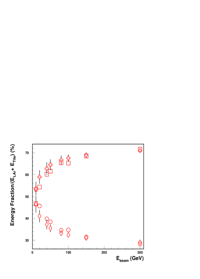
Figure 10: Energy deposition (percentage) in the LAr and Tile calorimeters at different beam energies. The circles (squares) are the measured energy depositions in the LAr (Tile) calorimeter, the diamonds (crosses) are the calculated energy depositions in the ones.

The obtained parameterization has some additional applications. For example, this formula may be used for an estimate of the energy deposition in various parts of a combined calorimeter. This demonstrates in Fig. 10 in which the measured and calculated relative values of the energy deposition in the LAr and Tile calorimeters are presented. The relative energy deposition in the LAr calorimeter decreases from about 50% at 10 $GeV$ to 30% at 300 $GeV$. On the contrary, the one in Tile calorimeter increases with the energy increasing.

5 Conclusions

Hadron energy reconstruction for the ATLAS barrel prototype combined calorimeter, consisting of the lead-liquid argon electromagnetic part and the iron-scintillator hadronic part, in the framework of the non-parametrical method has been fulfilled. The non-parametrical method of the energy reconstruction for a combined calorimeter uses only the known $e/h$ ratios and the electron calibration constants, does not require the determination of any parameters by a minimization technique and can be used for the fast energy reconstruction in the first level trigger. The correctness of the reconstruction of the mean values of energies (for energy biger than 10 GeV) within $\pm 1\%$ has been demonstrated. The obtained fractional energy resolution is $[(58\pm 3)\%\sqrt{GeV}/\sqrt{E}+(2.5\pm 0.3)\%]\oplus(1.7\pm 0.2)\ GeV/E$. The obtained value of the $e/h$ ratio for electromagnetic compartment of the combined calorimeter is $1.74\pm 0.04$ and agrees with the prediction that $e/h>1.7$ for this electromagnetic calorimeter. The results of the study of the longitudinal hadronic shower development are presented. The data have been taken on the H8 beam of the CERN SPS, with the pion beams of 10 – 300 GeV.

6 Acknowledgments

This work is the result of the efforts of many people from the ATLAS Collaboration. The authors are greatly indebted to all Collaboration for their test beam setup and data taking. Authors are grateful Peter Jenni for fruitful discussion.

Table 1: Mean reconstructed energy, energy resolution and fractional energy resolution for the various beam energies.

$E_{beam}$	$E$ (GeV)	$\sigma$ (GeV)	$\sigma/E\ (\%)$
$10^{\ast}$ GeV	$9.30\pm 0.07$	$2.53\pm 0.05$	$27.20\pm 0.58$
$20^{\star}$ GeV	$19.44\pm 0.06$	$3.41\pm 0.06$	$17.54\pm 0.31$
40 GeV	$39.62\pm 0.11$	$5.06\pm 0.08$	$12.77\pm 0.21$
50 GeV	$49.85\pm 0.13$	$5.69\pm 0.13$	$11.41\pm 0.26$
80 GeV	$79.45\pm 0.16$	$7.14\pm 0.14$	$8.99\pm 0.18$
100 GeV	$99.10\pm 0.17$	$8.40\pm 0.16$	$8.48\pm 0.16$
150 GeV	$150.52\pm 0.19$	$11.20\pm 0.18$	$7.44\pm 0.12$
300 GeV	$298.23\pm 0.37$	$17.59\pm 0.33$	$5.90\pm 0.11$
∗The measured value of the beam energy is 9.81 $GeV$.
⋆The measured value of the beam energy is 19.8 $GeV$.

Table 2: The differential energy depositions $\Delta E/\Delta x$ as a function of the longitudinal coordinate $x$ for the various beam energies.

N	x	$E_{beam}$ (GeV)
depth	($\lambda_{\pi}$)	10	20	40	50
1	0.294	$5.45\pm 0.08$	$8.58\pm 0.16$	$14.3\pm 0.2$	$16.6\pm 0.4$
2	0.681	$4.70\pm 0.08$	$9.10\pm 0.15$	$16.7\pm 0.2$	$20.8\pm 0.3$
3	1.026	$2.66\pm 0.06$	$5.55\pm 0.11$	$11.1\pm 0.2$	$13.6\pm 0.2$
dm	1.315	$1.35\pm 0.07$	$2.75\pm 0.14$	$5.28\pm 0.26$	$6.46\pm 0.32$
4	2.06	$1.93\pm 0.03$	$4.35\pm 0.06$	$8.99\pm 0.08$	$11.0\pm 0.1$
5	3.47	$0.87\pm 0.02$	$2.13\pm 0.04$	$5.29\pm 0.06$	$6.15\pm 0.10$
6	5.28	$0.18\pm 0.01$	$0.57\pm 0.02$	$1.50\pm 0.03$	$2.07\pm 0.05$
7	7.50	$0.025\pm 0.003$	$0.11\pm 0.01$	$0.32\pm 0.01$	$0.49\pm 0.02$
N	x	$E_{beam}$ (GeV)
depth	($\lambda_{\pi}$)	80	100	150	300
1	0.294	$22.6\pm 0.6$	$28.4\pm 0.6$	$36.3\pm 0.7$	$61.3\pm 1.5$
2	0.681	$30.4\pm 0.4$	$37.6\pm 0.5$	$53.5\pm 0.8$	$97.9\pm 1.7$
3	1.026	$20.3\pm 0.3$	$25.7\pm 0.4$	$37.2\pm 0.6$	$68.9\pm 1.2$
dm	1.315	$10.1\pm 0.5$	$12.8\pm 0.6$	$19.0\pm 1.0$	$34.1\pm 1.7$
4	2.06	$18.0\pm 0.1$	$22.4\pm 0.2$	$33.9\pm 0.3$	$64.8\pm 0.7$
5	3.47	$11.9\pm 0.1$	$14.6\pm 0.2$	$23.3\pm 0.2$	$49.0\pm 0.5$
6	5.28	$3.66\pm 0.06$	$4.57\pm 0.08$	$8.18\pm 0.13$	$18.6\pm 0.3$
7	7.50	$0.86\pm 0.03$	$1.10\pm 0.04$	$2.04\pm 0.06$	$5.54\pm 0.15$

Figure 2: The distributions of the $(e/\pi)_{LAr}$ ratio for $E_{beam}$ = 10, 20, 40, 50 GeV (top row, left to right) and $E_{beam}$ = 80, 100, 150, 300 GeV (bottom row, left to right).

Figure 6: The energy distributions for $E_{beam}$ = 10, 20, 40, 50 GeV (top row, left to right) and $E_{beam}$ = 80, 100, 150, 300 GeV (bottom row, left to right).

References

- [1] ATLAS Collaboration, ATLAS Technical Proposal for a General Purpose pp Experiment at the Large Hadron Collider, CERN/LHCC/94-93, CERN, Geneva, Switzerland.
- [2] ATLAS Collaboration, ATLAS TILE Calorimeter Technical Design Report, CERN/LHCC/96-42, ATLAS TDR 3, 1996, CERN, Geneva.
- [3] ATLAS Collaboration, ATLAS Liquid Argon Calorimeter Technical Design Report, CERN/LHCC/96-41, ATLAS TDR 2, 1996, CERN, Geneva, Switzerland.
- [4] F. Ariztizabal et al., NIM A349 (1994) 384.
- [5] A. Juste, ATL-TILECAL-95-69, 1995, CERN, Geneva, Switzerland.
- [6] J. Budagov, Y. Kulchitsky et al., ATL-TILECAL-96-72, 1996, CERN, Geneva, Switzerland.
- [7] Y. Kulchitsky et al., ATL-TILECAL-99-002, 1999, CERN, Geneva.
- [8] ATLAS Collaboration, Results from an Expanded Combined Test of the Electromagnetic Liquid Argon Calorimeter with a Hadronic Scintillating-Tile Calorimeter, Submitted to NIM A, 2000.
- [9] M. Cobal et al., ATL-TILECAL-98-168, 1998, CERN, Geneva.
- [10] D.M. Gingrich et al., (RD3 Collaboration), NIM A364 (1995) 290.
- [11] O. Gildemeister, F. Nessi-Tedaldi, M. Nessi, Proc. 2nd Int. Conf. on Calorimetry in High Energy Physics, Capri, 1991.
-
[12]
F. Ariztizabal et al., RD34 Collaboration, NIM (1994) 384;
E.Berger et al., RD34 Collaboration, CERN/LHCC/95-44. -
[13]
M. Bosman et al., RD34 Collaboration, CERN/DRDC/93-3, 1993;
F.Ariztizabal et al., RD34 Collaboration, CERN/DRDC/94-66, 1994. - [14] S. Agnvall et al., Hadronic Shower Development in Iron-Scintillator Tile Calorimetry, NIM A (in press).
- [15] J. Budagov, Y. Kulchitsky et al., ATL-TILECAL-97-127, 1997, CERN, Geneva, Switzerland.
- [16] R. Wigmans, NIM A265 (1988) 273.
- [17] D. Groom, Proceedings of the Workshop on Calorimetry for the Supercollides, Tuscaloosa, Alabama, USA, 1989.
- [18] Z. Ajaltouni et al., NIM A387 (1997) 333.
- [19] M. Bosman, Y. Kulchitsky, M. Nessi, ATL-COM-TILECAL-99-011, 1999, CERN, Geneva, Switzerland.
- [20] ATLAS Collaboration, ATLAS Physical Technical Design Report, v.1, CERN-LHCC-99-02, ATLAS-TDR-14, CERN, Geneva, Switzerland
- [21] R.Wigmans, Proc.2nd Int.Conf. on Calorimetry in HEP, Capri, 1991.
- [22] R. Bock et al., NIM 186 (1981) 533.
- [23] Y. Kulchitsky et al., NIM A413 (1998) 484.
- [24] Y. Kulchitsky et al., Submitted to NIM A, 2000.