Track Fit Hypothesis Testing and Kink Selection using Sequential Correlations

Abstract

Deviations between the form of trajectory assumed in a fit to a set of measurements and the actual form of the trajectory can give rise to sequential correlations in the residuals from the fit. These correlations can provide a more powerful goodness-of-fit test than that based on the minimum ${\mathrm{\chi^{2}}}$ from a least squares fit. The use of this additional information is explored in the context of several common trajectory errors (e.g. decays in flight) encountered in charged particle tracking.

and

1 Introduction

Trajectory fitting aims to determine a set of fitted parameters and to test the validity of the trajectory hypothesis. Both of these questions are usually addressed by minimizing a ${\mathrm{\chi^{2}}}$ constructed from the squares of the deviations between the measurements and the parameterized trajectory. The value of ${\mathrm{\chi^{2}}}$ at the minimum is used to test the adequacy of the fitted hypothesis.Cowan The ${\mathrm{\chi^{2}}}$ test, however, explicitly ignores correlations amongst the residuals from the fit. Such correlations arise naturally in trajectory fitting, where adjacent measurements are in causal order. Deviations from the expected trajectory due to either a discrete change at some point (e.g. a scattering or decay in flight) or to a continuous parameter change (e.g. dE/dx energy loss or magnetic field anomalies) introduce correlated shifts in the positions of all subsequent measurements. The ${\mathrm{\chi^{2}}}$ test is not very sensitive to these trajectory deviations when they are small on the scale of the measurement errors, since it considers only the squares of the residuals.

This paper introduces new quantities for hypothesis testing that are applicable to any fits for which an ordering variable (e.g. time) can be identified. The mean correlation of ordered sets of residuals (nearest neighbor, next nearest neighbor, etc.) are used for this purpose. These correlations are essentially independent of ${\mathrm{\chi^{2}}}$, and test the assumption that the measurements are mutually independent (or, more generally, that the correlations amongst the measurements are properly accounted for in the fit). It should be noted that the presumption of the independence of the measurements once known sources of correlation (e.g. multiple Coulomb scattering) are taken into account is also present in sequential fitting methods such as the Kalman FilterKalman , Fruhwirth , and the correlation test developed here can be applied to the output of such a fit.

The power of these correlation statistics for hypothesis testing is studied as a function of several trajectory deviations that arise naturally in charged particle tracking. For simplicity, the trajectories studied are circular arcs, corresponding to the projection of charged particle trajectories onto a plane transverse to a uniform axial magnetic field. The following sections describe the correlation variables, the simulation used to measure their effectiveness, and the improvement in discrimination between true and false hypotheses beyond what can be achieved using ${\mathrm{\chi^{2}}}$ alone.

2 Description of correlation variables

The degree to which nearby measurements are correlated can be gauged by considering the mean correlation as a function of the distance between measurements. Using the standard correlation estimatorCowan to form an average correlation

$${\mathrm{r_{k}={\sum_{i}\frac{\delta_{i}\,\delta_{i+k}}{\sigma_{i}\,\sigma_{i+k}}}\ /\ {\sqrt{\left(\sum_{i}\frac{\delta_{i}^{2}}{\sigma_{i}^{2}}\right)\left(\sum_{i}\frac{\delta_{i+k}^{2}}{\sigma_{i+k}^{2}}\right)}}}}$$ (1)

as a function of the distance between measurements gives fairly good discrimination between true and false trajectory hypotheses. The sums run from 1 to ${\mathrm{N-k}}$, ${\mathrm{N}}$ is the number of measurements on the trajectory, ${\mathrm{\delta_{i}}}$ is the signed distance to the fitted trajectory for measurement ${\mathrm{i}}$, ${\mathrm{\sigma_{i}}}$ is the estimated uncertainty of measurement ${\mathrm{i}}$, and ${\mathrm{k}}$ is the correlation distance: ${\mathrm{k\in[1,N-1]}}$. However, the following combination,

$${\mathrm{\rho_{k}={\sum_{i}w_{i}\frac{2\,\delta_{i}\,\delta_{i+k}}{\delta_{i}^{2}+\delta_{i+k}^{2}}}\ /\ {\sum_{i}w_{i}}\ \,;\ \ w_{i}=\frac{\delta_{i}^{2}+\delta_{i+k}^{2}}{\sigma_{i}^{2}+\sigma_{i+k}^{2}}}}$$ (2)

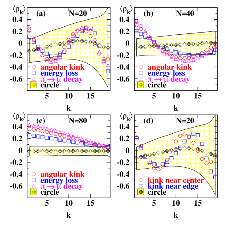
Figure 1: The expectation value of the correlation variable ${\mathrm{\rho_{k}}}$ is shown as a function of the correlation length ${\mathrm{k}}$. The first 19 ${\mathrm{\langle\rho_{k}\rangle}}$ are shown for 20 (a), 40 (b) and 80 (c) measurements. The different symbols correspond to specific generated trajectories; the fitted trajectory is a circle in each case. The shaded region indicates the r.m.s. of the ${\mathrm{\rho_{k}}}$ distribution for the circle trajectory. (d) shows ${\mathrm{\langle\rho_{k}\rangle}}$ for angular kinks occurring at different locations.

motivated by considering the measure ${\mathrm{(\delta_{i}-\delta_{i+k})^{2}\,/\,(\sigma_{i}^{2}+\sigma_{i+k}^{2})}}$, gives slightly better discrimination. This is because the correlation sought is in the actual distances ${\mathrm{\delta}}$ from the fitted trajectory, not in the residuals ${\mathrm{\delta/\sigma}}$. The weight factor emphasizes those pairs of measurements with significant deviations. These correlation measures satisfy ${\mathrm{\left|\rho_{k}\right|\leq 1}}$ for all ${\mathrm{k}}$. For uncorrelated measurements the expectation values of the ${\mathrm{\rho_{k}}}$ are close to zero. Negative correlations are introduced by the trajectory fit; they are small provided the number of fitted parameters is much smaller than the number of measurements.

Fig. 1(a-c) shows the expectation value of each ${\mathrm{\rho_{k}}}$ as a function of the correlation distance k (for ${\mathrm{k}}$ up to 19) for true circle trajectories and for three common trajectory deviations: a discrete angular kink, an uncorrected continuous energy loss and the decay in flight of a pion to a muon. The locations of the angular kink and decay in flight were uniformly distributed along the trajectory. The fitted trajectory in each case was a circular arc. The magnitudes of the ${\mathrm{\langle\rho_{k}\rangle}}$ for the incorrect hypotheses depend on the particular choice of parameters in the simulation. The number and location of the crossing points between ${\mathrm{\langle\rho_{k}\rangle}}$ for the incorrect trajectory hypotheses and ${\mathrm{\langle\rho_{k}\rangle}}$ for the correct hypothesis are very similar for the trajectory deviations studied here. Fig. 1(d) compares a sample with a discrete angular kink located near the center of the measurement region with a sample where the kink is located closer to the edge of the measurement region. The kink location clearly has an impact on the behavior of ${\mathrm{\langle\rho_{k}\rangle}}$, most notably for large ${\mathrm{k/N}}$.

Using all of the ${\mathrm{\rho_{k}}}$ values gives the best discrimination between the correct hypothesis and a particular type of incorrect hypothesis, but does not provide optimal discrimination for all types of incorrect hypothesis as can be seen by considering the different shapes (note in particular the locations of the extrema) of the trajectory hypotheses shown in Fig. 1. Furthermore, most of the discrimination power is concentrated at small ${\mathrm{k}}$, since the r.m.s. of the ${\mathrm{\rho_{k}}}$ distributions expected for the correct hypothesis are smallest there. These considerations, along with the essentially linear behavior of the difference ${\mathrm{\langle\rho_{k}\rangle_{false}-\langle\rho_{k}\rangle_{true}}}$ as a function of the correlation distance ${\mathrm{k}}$ for small ${\mathrm{k/N}}$, lead us to the following test statistic:

$${\mathrm{\lambda=\sum_{k=1}^{L}C_{k}\rho_{k}\ with\ C_{k}=\frac{2}{L(L-1)}(L-k)\ \ and\ \sum_{k=1}^{L}C_{k}=1}}.$$ (3)

Choosing ${\mathrm{L}}$ as the nearest integer to ${\mathrm{N/8}}$ was found to give good sensitivity to the trajectory deviations studied.

3 Description of simulation

The sensitivity of ${\mathrm{\lambda}}$ to trajectory deviations was studied using a simple simulation. Charged particles were generated and tracked through a uniform axial magnetic field and measured points were generated in the plane orthogonal to the magnetic field direction. The measurement uncertainty was taken as Gaussian. Trajectories were generated with parameters typical of charged particle tracking detectorsbabartdr :

• average hit resolution: 150 ${\mathrm{\mu m}}$;

• variation in resolution: factor of 5 between the best and worst measured points;

• radial difference between first and last measurement layer: 54 cm;

• number of measurements: varied from 20 to 160;

• magnetic field: axial field of magnitude 1.5 Tesla;

• initial particle momentum between 0.5 GeV/c and 5 GeV/c.

The measurements were uniformly distributed along the trajectories, the hit efficiency was unity and no noise hits were generated. The location of discrete trajectory deviations (angular kink or particle decay) was randomly distributed along the trajectory. The generated points were fitted to a circle assuming perfect pattern recognition, i.e. all generated measurements were used in the fit.

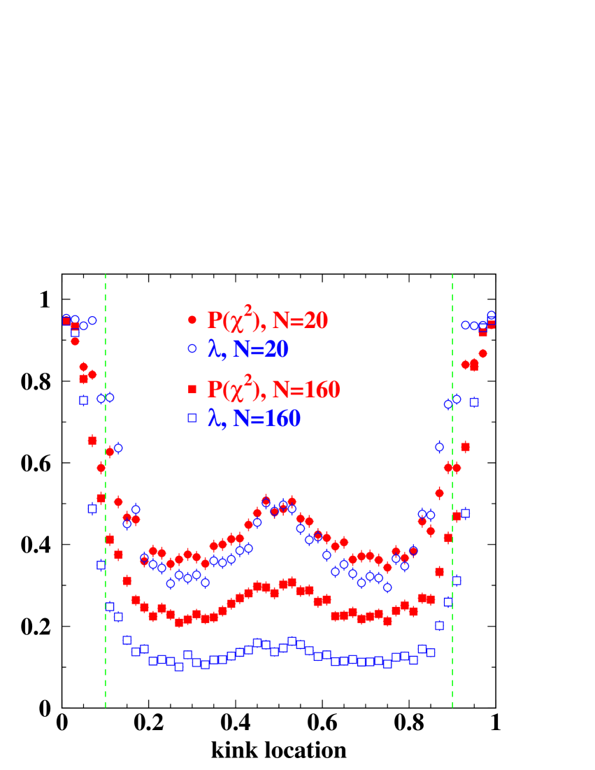
Figure 2: The survival rate as a function of the location of a discrete angular kink within the measurement volume. The cuts on ${\mathrm{\lambda}}$ and ${\mathrm{P(\chi^{2})}}$ are set to give 95% efficiency for true circular trajectories. The dashed lines bound the region used for subsequent study of the power of each variable.

4 Results

The generated data were used to study the discrimination power of ${\mathrm{\lambda}}$ and of ${\mathrm{\chi^{2}}}$ as a function of specific trajectory deviations. Fig. 2 shows the fraction of trajectories surviving a cut on ${\mathrm{\lambda}}$ or on the ${\mathrm{\chi^{2}}}$ probability ${\mathrm{P(\chi^{2})}}$ as a function of the position of a discrete angular kink, where the kink angle was uniformly distributed between ${\mathrm{\pm 0.02}}$ radians. The cuts were set to give 95% efficiency for true circular trajectories. There is little discrimination power for kinks occurring at either end of the measurement region. Based on this, only those trajectory deviations occurring within a fiducial region consisting of the central 80% of the measurements were selected for subsequent study.

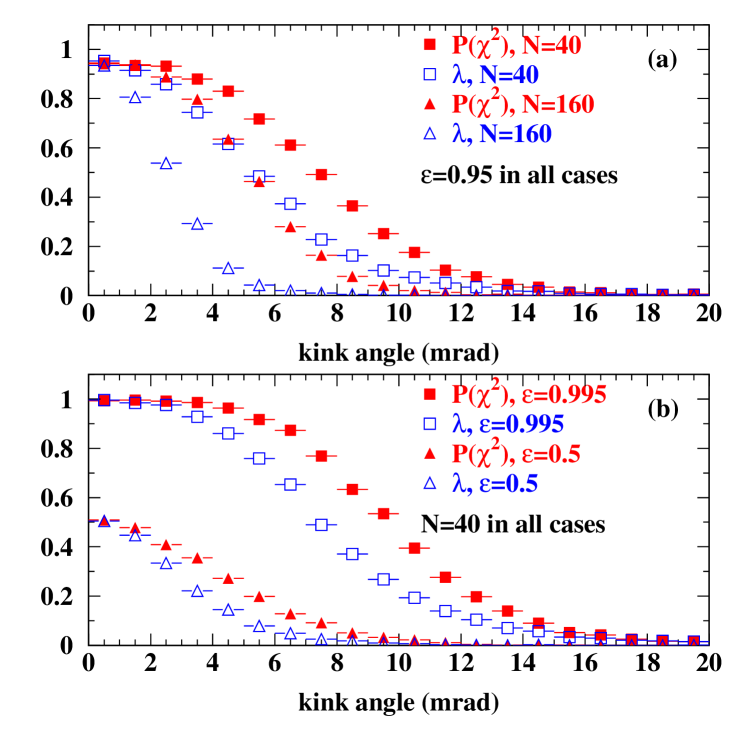
Figure 3: The survival rate as a function of the size of a discrete angular kink within the fiducial region. The behavior for different N is shown in (a) for a cut that gives an efficiency ${\mathrm{\epsilon}}$ of 95% for true circular trajectories. The curves in (b) show the effect of varying the cut on ${\mathrm{\epsilon}}$.

The fraction of these selected trajectories surviving a cut that gives 95% efficiency for true circular trajectories is shown as a function of the size of the angular deviation in Fig. 3. The correlation variable ${\mathrm{\lambda}}$ is more powerful than ${\mathrm{P(\chi^{2})}}$ provided ${\mathrm{N>20}}$ and becomes relatively more powerful as the number of measurements increases. This is to be expected, since the physical correlation length sampled by ${\mathrm{\lambda}}$ is of the order of ${\mathrm{\frac{1}{8}}}$ of the track length, and increasing the density of measurements allows a more precise determination of the correlation. Similar behavior is observed for different choices for the efficiency for true circular trajectories. The power of ${\mathrm{\lambda}}$ and ${\mathrm{P(\chi^{2})}}$ to discriminate ${\mathrm{\pi\rightarrow\mu}}$ decays from true circular trajectories is shown in Fig. 4. Note that the decay angle between the

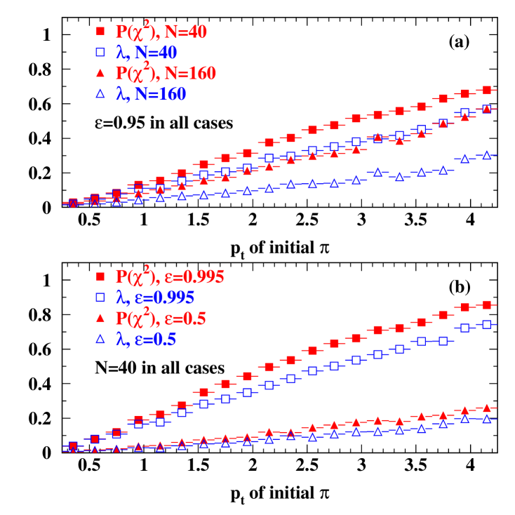
Figure 4: The survival rate for ${\mathrm{\pi\rightarrow\mu}}$ decays occurring in the fiducial region as a function of the initial momentum of the pion in the plane transverse to the magnetic field. The behavior for different N is shown in (a) for a cut that gives an efficiency ${\mathrm{\epsilon}}$ of 95% for true circular trajectories. The curves in (b) show the effect of varying the cut on ${\mathrm{\epsilon}}$.

${\mathrm{\pi}}$ and ${\mathrm{\mu}}$ does not in general lie in the measurement plane, and that the momentum of the muon will be smaller than that of the pion. The correlation variable ${\mathrm{\lambda}}$ is again a significantly better discriminant than is ${\mathrm{P(\chi^{2})}}$.

The extent to which the discrimination afforded by ${\mathrm{\lambda}}$ is optimal was studied. The measurements along trajectories generated with a discrete angular kink were fitted using both the correct hypothesis, i.e. two circular arcs of constant curvature with an angular deviation at a point, and using the nominal (incorrect) hypothesis of a single circular arc. The ratio of the resulting ${\mathrm{\chi^{2}}}$ probabilities ${\mathrm{P_{circle}(\chi^{2})/P_{correct}(\chi^{2})}}$ is an optimal discriminant variable in this case. The position of the angular kink was taken as either the true position of the generated deviation (denoted “fixed ${\mathrm{R_{kink}}}$” in Fig. 5) or as the best fit value after considering all

Figure 5: The survival rate as a function of the size of a discrete angular kink for 40 (a) and 160 (b) measurements. The cuts on ${\mathrm{\lambda}}$ and ${\mathrm{P(\chi^{2})}}$ are set to give 95% efficiency for true circular trajectories. Also shown are results from an optimal technique (see text) with the kink location either fixed to the generated position (“fixed ${\mathrm{R_{kink}}}$”) or determined by the fit (“fitted ${\mathrm{R_{kink}}}$”).

potential kink positions (denoted “fitted ${\mathrm{R_{kink}}}$” in Fig. 5). The kink position will in general be unknown, so the “fitted ${\mathrm{R_{kink}}}$” curve is in practice the best one can achieve. As is seen in Fig. 5, the correlation variable ${\mathrm{\lambda}}$ gives discrimination that approaches the optimal value as the number of measurements increases.

5 Discussion

The correlation variables ${\mathrm{\rho_{k}}}$ introduced here test the assumption that a set of measurements are mutually independent once known sources of correlation have been taken into account. Use of the simple combination of ${\mathrm{\rho_{k}}}$ introduced here as ${\mathrm{\lambda}}$ leads to an improvement in the sensitivity for detecting small trajectory deviations relative to that achievable using ${\mathrm{P(\chi^{2})}}$. This additional goodness-of-fit test is independent of the ${\mathrm{\chi^{2}}}$ test, and can be applied to the residuals from both traditional least squares fits and from Kalman filter fits. The improved sensitivity to small deviations can be qualitatively understood by recognizing that ${\mathrm{\chi^{2}}}$ has a quadratic dependence on individual deviations, while ${\mathrm{\lambda}}$ has a linear dependence. For larger deviations (not shown here) ${\mathrm{P(\chi^{2})}}$ becomes a more powerful discriminant than ${\mathrm{\lambda}}$, as expected. For the deviations studied, the gain from combining the ${\mathrm{\lambda}}$ and ${\mathrm{P(\chi^{2})}}$ tests was negligible.

The ${\mathrm{\lambda}}$ and ${\mathrm{\chi^{2}}}$ tests have different dependencies on the input to the fit. The ${\mathrm{\chi^{2}}}$ test is sensitive to the scale of the assigned measurement errors ${\mathrm{\sigma_{i}}}$ and can be compromised by mis-estimates of and non-Gaussian contributions to the measurement errors. The ${\mathrm{\lambda}}$ test is insensitive to the scale of the ${\mathrm{\sigma_{i}}}$. It is, however, sensitive to correlations introduced in calibration procedures. The extent to which this is a practical problem in using the ${\mathrm{\lambda}}$ test is a function of detector design and calibration. In particular we expect the ${\mathrm{\lambda}}$ test to be most useful in devices where the effect of calibrations is randomized over the measurements on a trajectory (e.g. in small cell drift chambers, where the drift direction changes layer by layer), and to be less effective in devices where coherent effects dominate (e.g. in detectors employing a jet cell design).

Potential uses for the ${\mathrm{\lambda}}$ test in charged particle tracking involve selecting decays in flight and enabling high quality track samples (with reduced non-Gaussian tails on the track parameter resolutions due to trajectory deviations) to be selected. Given the ease with which it can be calculated, a test on ${\mathrm{\lambda}}$ might serve as a filter for selecting tracks on which more computationally intensive testsFruhwirth , Cousins will be performed. The correlations measured by the ${\mathrm{\rho_{k}}}$ parameters may find use in a broader range of applications.

6 Acknowledgments

The authors would like to thank Dr. Michael Roney for useful discussions and to acknowledge Louis Desroches, whose work with one of us (Kowalewski) on run test variables was a precursor to the present work.

References

- [1] See, e.g., G. Cowan, Statistical Data Analysis. Clarendon Press, Oxford, 1998.
- [2] P. Billoir, Nucl. Instr. Meth. 255 (1984) 352; P. Billoir, R. Frühwirth and M. Regler, Nucl. Instr. Meth. A241 (1985) 115-131.
- [3] R. Frühwirth, Nucl. Instr. Meth. 262 (1987) 444.
-
[4]
This particular choice is close to those given in the
BABAR Technical Design Report, available at
http://www.slac.stanford.edu/BFROOT/www/doc/TDR/ - [5] P. Astier et al., “Kalman Filter Track Fits and Track Breakpoint Analysis,” e-Print Archive physics/9912034.