Radio-Frequency Measurements of
Coherent Transition and Cherenkov Radiation:
Implications for High-Energy Neutrino Detection

Abstract

We report on measurements of 11-18 cm wavelength radio emission from interactions of 15.2 MeV pulsed electron bunches at the Argonne Wakefield Accelerator. The electrons were observed both in a configuration where they produced primarily transition radiation from an aluminum foil, and in a configuration designed for the electrons to produce Cherenkov radiation in a silica sand target. Our aim was to emulate the large electron excess expected to develop during an electromagnetic cascade initiated by an ultra-high-energy particle. Such charge asymmetries are predicted to produce strong coherent radio pulses, which are the basis for several experiments to detect high-energy neutrinos from the showers they induce in Antarctic ice and in the lunar regolith. We detected coherent emission which we attribute both to transition and possibly Cherenkov radiation at different levels depending on the experimental conditions. We discuss implications for experiments relying on radio emission for detection of electromagnetic cascades produced by ultra high-energy neutrinos.

(To be published in Physical Review E)

I Introduction

In 1962, G. Askaryan[1] first predicted that large electromagnetic particle cascades would develop an asymmetry of electrons over positrons at the level of 20-30% due to the following processes: Compton scattering of atomic electrons in the target material by cascade photons, $\delta$-ray scattering processes, and annihilation of positrons in flight. Askaryan realized that the propagation of this charge asymmetry in a dielectric medium should result in radio emission due to the processes of Cherenkov and transition radiation. For wavelengths much larger than the shower dimensions, he noted that the radio emission would be coherent, i.e., the electrons radiate in phase, with a resulting $N_{e}^{2}$ increase in the radiated power with the number of excess electrons $N_{e}$, in contrast with a linear rise expected from incoherent emission.

Recently this suggestion has generated renewed interest both on experimental and theoretical fronts. On the experimental side, it has become the basis for a number of new searches for radio-frequency (RF) emission from cascades induced by ultra-high energy neutrinos—at PeV energies in Antarctic ice [2, 3, 4, 5] and at EeV energies from the lunar regolith [6, 7, 8, 9, 10]. On the theoretical side, a number of recent, very detailed simulations[6, 11, 12, 13] have validated Askaryan’s basic result: Particle cascades at energies from $\sim$1 TeV up to $10^{20}$ eV will develop a net negative charge excess of order 20-30% of their total charged-particle number. These simulations also confirm Askaryan’s prediction of a corresponding nanosecond pulse of radio Cherenkov emission, with a characteristic frequency and angular dependence. Extending Askaryan’s original idea, Markov and Zheleznykh [14] have also shown that a number of other coherent radiation processes, such as transition, synchrotron, and bremsstrahlung radiation, are likely to be important contributors to the total emission from cascades depending on the cascade medium, ambient fields, and geometry.

A Experimental tests

Under typical conditions, none of these processes produce radio emission comparable to that of other passbands until the energy of the cascades exceeds $\sim 10^{15}$ eV. Thus a direct accelerator beam test of these predictions is difficult. Such a test could be made with existing TeV proton beams where observations of radio emission, though expected to be correspondingly weak and difficult to characterize, would demonstrate the existence of the charge asymmetry. However, a failure to detect radio emission under these circumstances might be attributable to either a failure of the shower to produce the predicted charge asymmetry, or a loss of radio coherence in the emission process after the charge asymmetry has developed.

As an alternative experimental approach, we have utilized lower energy pulsed electron bunches incident on a target material. The electron bunch then emulates the resulting charge asymmetry from the late stages of a high energy cascade, and allows one to focus experimentally on the radio emission process. Simulations have shown[11] that the bulk of the radio emission arises from low-energy electrons ($\leq 10$ MeV) produced late in the shower. Thus investigations of the coherent radio emission properties can be done with fairly modest electron energies, provided that the bunch length is at least as small as the longitudinal and transverse shower sizes expected in cascades in solid materials (several cm). The total number of charged particles, (which are virtually all electrons and positrons near and after shower maximum) in a cascade is to a good approximation $E_{shower}/\mbox{GeV}$. Hence, a given cascade energy can be simply related to the number of electrons per pulse at an accelerator.

We have adopted this alternative approach to begin developing a laboratory basis for confirmation of Askaryan’s hypothesis. Using the Argonne Wakefield Accelerator (AWA) facility at Argonne National Laboratory, we have employed $20-50$ ps pulsed electron bunches with $N_{e}\simeq 10^{10-11}$ electrons per bunch to produce coherent radio emission from several targets. We looked for radio emission in the 1.7–2.6 GHz microwave band (11-18 cm wavelength). Our initial measurements show evidence for both coherent transition and perhaps Cherenkov radiation. In the following section we discuss some of the history of related measurements at other facilities. Section II gives a summary of the theoretical basis for the emission. In section III we describe our experimental setup, the measurements made, and the results obtained. We conclude the paper by considering the applications of these results to coherent radio detection of neutrino-induced cascades.

B Related measurements of coherent emission from LINAC beams

Over the last two decades a significant effort has gone into measurements of coherent Cherenkov radiation (CR) and transition radiation (TR) from electron linear accelerator (LINAC) beams. The primary motivation for these experiments has been the development and characterization of coherent sources of millimeter-wave and far-infrared radiation. Although several early experiments [15, 16] were done at centimeter wavelengths using continuous-beam devices, most recent work has focussed on the shorter wavelengths. In the early cm-wave work the detected power was attributed to CR from air at the end of the beam pipe. No measurements of the coherence properties were made.

Later work [17, 18, 19] demonstrated the coherence of radiation observed under similar conditions, again attributing it in part to CR. Following this, a number of authors[18, 20, 21] realized that the bulk of the observed radiation in such circumstances must in fact be primarily TR, and that the Cherenkov contribution was not easily separable given the experimental configurations used. This is primarily due to two features of these experiments: First, the Cherenkov angular distribution in air is nearly identical to that of TR. Second, the relatively short effective path-lengths of the electron beam in the air meant that the CR power was suppressed compared to the TR power.

II Theoretical considerations

As we have noted above, the primary radio emission processes that we expect to be important in our experiment are transition and Cherenkov radiation. Both of these processes are well-known and studied in the optical (for CR) and X-ray (for TR) regimes, but the emission is not typically coherent at these wavelengths. In addition, most CR emission is observed under conditions where the emitting region and the charged-particle track length is physically much longer than the wavelength observed; for our accelerator experiments this condition is not satisfied and the traditional treatment of CR through the Frank-Tamm formulation, which obtains when the track length is much longer than the wavelength of observation, is not valid. In the case of transition radiation, most present work centers on the use of X-ray TR as a diagnostic for particle energies in detector systems at accelerators or in cosmic-ray detectors. A number of the approximations used for X-ray TR are not valid for radio emission, and our treatment here reflects that.

A Transition radiation

Transition radiation occurs as relativistic electrons cross the boundaries between dielectric media. The forward angular spectrum of TR for passage of a single electron through a single dielectric boundary with dielectric constants and indices of refraction $\epsilon_{1},n_{1}$ upstream and $\epsilon_{2},n_{2}$ downstream is given by [22, 20]:

$$\frac{d^{2}W_{TR}}{d\omega d\Omega}~{}=~{}\frac{\hbar\alpha}{\pi^{2}}\frac{\sqrt{\epsilon_{2}}\sin^{2}\theta\cos^{2}\theta}{(1-\beta^{2}\epsilon_{2}\cos^{2}\theta)^{2}}\ |\zeta|^{2}$$ (1)

where the angle $\theta$ is measured with respect to the electron direction, $\beta=v/c$ is the electron velocity, and $\hbar$ and $\alpha$ are Planck’s constant (over $2\pi$) and the fine-structure constant, respectively. The factor $\zeta$ is

$$\zeta~{}=~{}\frac{(\epsilon_{2}-\epsilon_{1})(1-\beta^{2}\epsilon_{2}-\beta\sqrt{\epsilon_{1}-\epsilon_{2}\sin^{2}\theta})}{(\epsilon_{1}\cos\theta+\sqrt{\epsilon_{2}}\sqrt{\epsilon_{1}-\epsilon_{2}\sin^{2}\theta})(1-\beta\sqrt{\epsilon_{1}-\epsilon_{2}\sin^{2}\theta})}$$ (2)

The equation is written this way since the factor $|\zeta\cos\theta|$ is close to unity for most solid–vacuum interfaces. We have neglected the magnetic permeability of the two media since it is unimportant for the materials in our experiment. The quantity expressed is the total radiated energy per unit radian frequency per unit solid angle. The dielectric constants $\epsilon_{i}$ are in general complex with both refractive and absorptive components. These equation show that the TR is forward-peaked with a characteristic angle $1/\gamma$ and that the radiation is broadband. Analogous results can be obtained for the backwards emission by multiplying by the appropriate Fresnel reflection coefficient. We refer the reader to the literature [22, 23, 24] for details.

We note that these results are derived for the case of a particle traversing from $-\infty$ and do not account for deceleration of the particle at the interfaces or in the media. These equations contain poles at several values of $\theta$ and $\epsilon_{2}$, most notably at the value of $\theta$ defined by

$$\cos\theta=(\beta\sqrt{\epsilon_{2}})^{-1},$$ (3)

which is the condition normally associated with the definition of the Cherenkov angle. This has been identified as an artifact of the assumption of an infinite medium and track length [22, 23], but it does highlight the close association of the TR and CR processes, and the complications that arise in separating them. As a result, equation 1 does not provide a clear theoretical distinction which would allow us to separate out the assumptions of an infinite medium and track length, in order to isolate the TR from the CR contribution. We discuss this issue further in appendix A.

Another important feature of transition radiation is its formation zone $L_{f}$  [22], which is the downstream region of the medium over which the radiation field due to the transition becomes fully separated from the coulomb field of the propagating charge. For fully-formed TR to develop, the dielectric boundary must be sharp compared to the size of this region, given by

$$L_{f}~{}=~{}{2\pi\beta c\over|\omega(1-n_{2}\beta\cos\theta)|}.$$ (4)

This also means that any effect which disturbs the dielectric properties of the downstream medium within the formation zone will tend to suppress the full formation of TR according to the equations developed above. For the case where the particle is stopped within the formation zone, the assumption used in developing the TR formalism are again not satisfied and we expect that the TR is again suppressed. At present the magnitude of this expected suppression is not quantified in the literature, but we note this effect since it is likely to be important at some level in our experiment.

B Cherenkov radiation

Cherenkov radiation from a finite electron track length is treated by Tamm[25], and discussed more recently in the context of coherent radiation from a LINAC beam by Takahashi et al.[20] For electrons traversing a track of length $L$ in a medium of index of refraction $n$ [20]:

$${d^{2}W_{\mbox{CR}}\over d\lambda d\Omega}~{}=~{}{hc\alpha n\over\lambda^{2}}\left({L\over\lambda}\right)^{2}\mbox{sinc}^{2}X(\lambda,\theta)~{}\sin^{2}\theta.$$ (5)

Here $\mbox{sinc}\ x\equiv\mbox{sin}\pi x/\pi x$ and

$$X(\lambda,\theta)~{}=~{}{L\over\beta\lambda}(1-\beta n\cos\theta),$$ (6)

where $\lambda$ is the wavelength of the radiation. The quantity expressed is the total radiated energy per unit wavelength per unit solid angle. As a result, the CR is peaked at a characteristic Cherenkov angle $\cos\theta_{C}=(\beta n)^{-1}$.

As we have noted above, the treatments of TR in the literature often contain elements that appear as limiting cases of a Cherenkov-like contribution. In fact similar statements can be made about treatments of Cherenkov radiation for the case of a finite track length. Takahashi et al.[20] have shown that this relation can be interpreted in terms of a CR-like component from the continuous portion of the track added to TR-like components from the end-points of the track. We have not attempted to make such a distinction, but we note again the strong physical connection between TR and CR.

C Coherent emission from electron bunches

The equations presented above have not explicitly treated the effects of coherence on the emission process. There is however an extensive literature describing the coherence properties of radiation from electron bunches[26, 21, 20]. As long as the transverse size of the bunch is less than a fraction of the wavelengths observed, the electric fields of each radiating electron add in phase and the net electric field grows linearly with the number of electrons, implying a quadratic growth of power. Thus for $N_{e}$ electrons per bunch, we expect the total radiated energy be $N_{e}^{2}$ times the formulas given above for single electrons.

This is the condition for full coherence, and it will only obtain in the limit where the bunch size is far smaller than the wavelength observed. In our case, although this condition is generally satisfied, there are corrections due to the bunch form factor which should be accounted for. This is typically done by introducing the form factors for the longitudinal, transverse, and angular emittance of the electron bunch:

$$P~{}=~{}N_{e}(1+N_{e}f_{L}f_{T}f_{\chi})P_{0}~{}.$$ (7)

Here $P$ is the radiated power, $f_{L},f_{T},f_{\chi}$ are the longitudinal, transverse, and angular emittance form factors, and $P_{0}$ the single-particle radiated power[20]. The spatial form factors can be estimated via a three-dimensional Fourier transform of the electron distribution (here assumed to have cylindrical symmetry); the angular form factor is somewhat more complex but can also be numerically evaluated if an estimate of the angular emittance of the beam is available[20].

III Experiment

Our experiment, although limited in part by some of the same effects as earlier works in separating coherent TR from CR, has been designed so that the Cherenkov angular distribution is quite distinct from the forward-peaked TR distribution. To do this we use silica sand as our target medium. This has the further advantage of being a more relevant medium with respect to the ongoing high energy neutrino experiments, since the material is comparable in refractive index and RF attenuation properties to both ice and the lunar regolith. It has the disadvantage of stopping a lower-energy electron shower relatively quickly, and this tends to weaken the resulting CR emission relative to that of TR, because of the $L^{2}$ dependence of the CR power on path length evident in equation 5 above.

A Electron beam

The Argonne Wakefield Accelerator (AWA)[27] at Argonne National Laboratory provided our electron bunches. AWA produces electron bunches of mean energy 15.2 MeV, and a bunch length of $\sim 1$ cm. The transverse distribution at the exit to the beam pipe was Gaussian with $\sigma\approx 7$ mm. The beam was pulsed once per second with a beam current tunable from 0.5 to 25 nC/pulse. The beam current was measured bunch-by-bunch using an integrating current transformer (ICT). The ICT produced an output voltage pulse proportional to the measured bunch charge which was recorded event-by-event.

B Target

The target geometry is shown in Fig. 1. The target consisted of a 80 cm diameter by 55 cm high polyethylene tub (wall thickness $\sim$3 mm) with a 6 inch diameter, schedule 40 PVC pipe penetrating its side. We used an empty tub for our initial runs with the PVC pipe left open on both ends. Thus the beam exited the accelerator through a 3 mil aluminum window and ranged out in air several meters beyond the experiment.

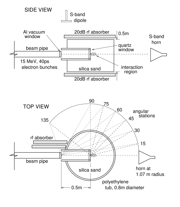
FIG. 1.: Two sectional views of the target geometry.

In subsequent runs, we filled the tub with 360 kg of silica sand, to within 7 cm of its top. The grain sizes were fairly uniform with 300 $\mu$m diameters. The average density (including the packing factor) was 1.58 g/cm³. We measured the index of refraction of the sand at 2 GHz to be $1.55\pm 0.01$, indicating that the water content was less than 3% by weight. [28] The attenuation of microwaves by 1 m of such dry sand is small, amounting to a loss of about 1.3 dB at 2 GHz. For the sand runs, the PVC pipe was capped with a quartz window at the internal end to hold in the sand. Our original intent was to lead the vacuum beam pipe into the center of the target but this proved impractical due to difficulties in adequately supporting the beam pipe. Thus the the electron bunches were transmitted through the aluminum vacuum window at the end of the beam pipe, through about 50 cm air, and entered the target through a quartz window of about 6 mm thickness.

We placed 20 dB of RF absorber above and below the tub to minimize reflections. To suppress RF emission from the TR at the beampipe into the backward direction, we generally ran with 20 dB of RF absorber along the side of the beampipe as shown in Fig.1.

C Simulation of expected electron shower

To characterize the expected shower behavior it was simulated using the EGS4 Monte Carlo [29] assuming that the material was quartz, but with the density adjusted to match that of the sand. This allowed us to estimate the longitudinal development in electron number as well as the elongation and lateral growth of the shower. The results of one such simulation are shown in Fig. 2. Here the curve marked $(N_{e-}-N_{e+})/N_{e-}^{inc}$ shows the evolution of the electron number as a small shower develops in the initial few cm, and then dies out, with a long tail of stragglers. The other two curves show the expected growth in the rms size in both transverse (Xrms) and longitudinal (Zrms) directions. Based on these results, we expect the CR emission in the sand to be primarily from the $\sim 3-4$ cm region of the shower maximum, with some additional contribution due to Compton electrons extending out to $\sim 20$ cm or more. This latter contribution is reduced due to the increase in the bunch size which decreases the coherence of radiation from this portion of the electron shower.

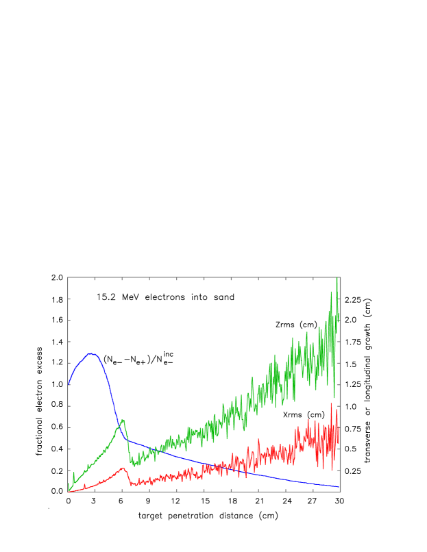
FIG. 2.: Simulation of the expected electron shower distribution for the 15.2 MeV electron bunch from the AWA facility, here done for quartz scaled for the lower density of sand used. The fractional number curve represents the net charge, accounting for the positrons produced. The change in rms bunch dimensions during propagation through the target is denoted by Zrms (longitudinal) and Xrms (transverse).

D Antennas

We received the RF emission signal using a pyramidal horn, with a nominal half-power bandpass of 1.7–2.6 GHz and directivity of 15.3 dB at 2.15 GHz. The rectangular aperture of the horn was 36.5 cm (E-plane) by 27.3 cm (H-plane). The angular response of the antenna is shown in Fig. 3. Phase errors at the front of the horn relative to its throat cause the effective area of a horn to be less than its geometric area. We calculated the ratio of effective aperture to geometric aperture to be 0.51, which is typical for such horns. Using a network analyzer we estimated further inefficiencies due to impedance mismatches and ohmic losses to be of order 10%. We estimate our ability to point the horn to be 5^∘, corresponding to a 2 dB loss on average.

FIG. 3.: Calculated angular response lobes of the pyramidal horn. The solid and dashed lines are for the H- and E-plane, respectively.

We used a balanced half-wave 6.9 cm dipole with a half-power bandwidth of $\sim 700$ MHz centered at 1.8 GHz to provide a trigger. The dipole signal had a risetime of $\sim 150$ ps and provided a trigger stable to 40 ps or better.

The antenna positions are shown in Fig. 1. The dipole was 50 cm from the exit of the beampipe at an angle of $70^{\circ}$ from the beam axis, and was stationary during the course of the experiment. The horn was moved along a fixed radius from the target center to a series of fixed angular positions from 0^∘ to 135^∘. The outputs of the two antennas were fed without amplification into 20 m of coaxial cables which brought the signals into the control room with a total attenuation of 6–7 dB.

As is typical for an accelerator experiment which must be done within the confines of a shielded vault, we were limited in our ability to place the antennas further than about 1-2 m from the source of the radiation. Thus the response of the horn will be affected by near-field (Fresnel zone) effects. The primary effect within the Fresnel zone is a loss of antenna efficiency due to wavefront curvature which produces a phase error across the receiving aperture. Using calculations in Ref [30], we estimate these effects to cause a 0.25-0.4 dB power loss, depending on the angle of the horn.

E Data acquisition

All measurements of pulsed RF emission were done in the time domain using a Tektronix 694C real-time digital sampling oscilloscope with 3 GHz bandwidth and 10 GS/s, 8-bit linear digitization of four channels. The signals from the horn and dipole required no amplification; in fact, because of the strength of the coherent radio emission, induced voltages in the antennas had to be limited by RF attenuators (typically 20 dB), to bring the signal into an acceptable range for the $50~{}\Omega$ scope inputs. The scope produces a time series of the voltages interpolated from 100 ps to 40 ps resolution, which is slightly faster than the input channel risetime, measured by Tektronix to be in the range of 50-60 ps. Thus we were able to sample the full bandwidth of the antenna outputs and thereby make direct measurements of the electric field intensities, mediated only by the response of the antennas and cables used. The excellent time resolution was useful for identifying spurious reflections from structures near the target. For each measurement, between 12 and 50 triggers were recorded. All of the recorded pulse profiles were far above ambient RF noise levels, and the pulse-to-pulse variation in the profiles is typically less than 5% per sample.

F Power and voltage measurements

Detected pulse energy at the face of the antenna was calculated by summing $4V^{2}/(50~{}\Omega)$ ($V$ is the measured voltage) over a 3 ns window (75 bins) defined by the primary radio pulse from the electron bunch, either from the Al window of the beampipe (for the TR runs) or the target center (for the CR runs). During this time window the power contributions from spurious reflections were negligible. The factor of 4 accounts for voltage dividing between the antenna and load. We measured the 3 ns time window to contain 98% of the total pulse energy as measured at the scope. The origin of the window was shifted to account for different propagation delays in the sand and air (1 ns). The raw recorded voltages were corrected directly for the effects of attenuators, cable and adaptor losses, near-field losses, transmission loss, aperture inefficiency, and pointing errors described above.

G Datasets

All of the data presented in this paper were taken over a two-day period, Sept. 23–24, 1999. Except for the “pure TR runs”, the measurements were taken 107.3 cm from the center of the tub with the horn pointing at the tub center.

• Pure TR runs: To establish the baseline TR contribution without possible CR effects from the target, we took data with the tub removed so that the only significant radiation would be TR from the aluminum beampipe vacuum window. Measurements were made with the horn at 8.5 and 16.6^∘, pointing directly at the aluminum window. The horn was placed 183 cm from the foil for these runs.

• Empty-target runs: Additional TR measurements were made using an empty target without the quartz window in place. Our initial goal here was to allow for the possibility of subtraction of the TR signal from the target-full runs; thus a complete set of angular measurements were made, under the same configurations as the full-target runs: that is, with the horn always pointing toward the target center. However, since there was neither any sand nor the quartz window present, the observed emission received by the horn actually emanates from the beampipe end. Emission of TR from the beampipe end is thus received off-axis by the horn at a given angular position, and must be corrected for the known beam response of the horn, which we have done.

  Measurements were taken at 15^∘ intervals from 15 to 135^∘. In addition measurements at the 45^∘ position were repeated at a range of beam currents to measure the coherence properties of the TR in our band.

• Full-target runs: With sand in the target, the electrons produce TR as they pass through the beampipe end, then both TR and CR as the enter the target. TR emission from the end of the beampipe will undergo refraction through the target. Refraction is less of an issue for CR and TR emission from the sand and quartz window, because we chose the cylindrical geometry to minimize such effects. However, any assessment of full-target contributions of the strong TR emission due to the beampipe end must account for for the refractive effects of the target.

  Measurements were taken at 15^∘ intervals from 0 to 135^∘. For a subset of angles we also measured the polarization of the radiation.

• Diagnostic runs: We took several special runs with strategically placed absorber sheets to allow for comparison studies of different portions of the observed time structure of the pulses. For example, we placed an absorber over the portion of the target viewed by the horn to allow us to identify multipath reception which was not directly associated with the target. Thus we identified unwanted reflections and eliminated them from consideration in the analysis.

IV Results

A TR measurements

To provide the simplest geometry for subsequent analysis of the TR emission, we made several runs without the large target present. To identify any possible emission from stray surface currents, diffraction, or image charge effects that might be induced by the beam along the beampipe, we made identical measurements in this sequence both with and without a $0.7\times 0.7$ m grounded piece of heavy Al foil several cm downstream from the vacuum window. The thickness of the foil (several mil) was well above the skin depth at our frequencies, and was intended to provide a TR radiator plane much larger than the wavelengths of interest.

FIG. 4.: Typical horn and dipole measured field strengths from TR produced at the beampipe end. (a),(b) Field strength from the horn are shown for two angles, with (c) showing the corresponding strength measured at the dipole, which was fixed in angle at $70^{\circ}$. The solid and dotted lines in (a) and (b) are from runs with and without a foil shield as described in the text.

Fig. 4 shows the measured field strengths for the two angles. The field strengths are corrected for attenuation and referenced to a distance of 1 m. Conversion of the measured voltages to field strengths requires a knowledge of the effective height of the antennas used; we estimated these to be 18 cm for the horn, and 7 cm for the dipole. The time axis is relative to the dipole trigger, shown in (c), which had a shorter cable length and was closer to the source. The emission with the large foil present is shown in solid lines, and that without the foil in the dotted lines. There is essentially no difference between the two. We conclude that there was no contribution due to unexpected image charge or other effects from the beampipe end.

TABLE I.: Measured and calculated pulse energies for the TR runs.

antenna	angle	measured energy	calculation	meas./calc.
	(∘)	($\mu$J/sr)	($\mu$J/sr)
horn	8.5	5.8	156.0	0.037
horn	16.6	1.7	45.5	0.037
dipole	70	21.6	3.3	6.25

There is a marked difference in the pulse shapes between the dipole and horn, which is likely to be due both to differences in the effective bandwidth of the two antennas and to partial impedance mismatches in the cables. However, in both cases the full-width at half maximum (FWHM) of the pulses is of order 1 ns, which indicates that the detected pulses are band-limited, since $\Delta T\simeq 1~{}{\rm ns}\simeq(\Delta f)^{-1}$. This is consistent with the view of TR as a process which arises very rapidly as the electrons cross a dielectric boundary, in this case from aluminum to air.

One might expect that there is some contribution to the measured pulse energy from CR along the air path within our acceptance angle. However, because the effective pathlength for CR production is fairly short in this case, and the microwave index of refraction of the air is close to unity, the CR contribution can be neglected with respect to the TR.

The fully corrected pulse energy measurements and those predicted by Equation 1, where we have assumed that the real part of the Al dielectric constant is $\epsilon_{r}=10$ at 2 GHz, are shown in Table I. For the horn measurements, the two are in disagreement by a factor of nearly 30. For the dipole, our single measurement at an angle of $70^{\circ}$ appears to give us more power than expected from the theory. As yet, the source of these discrepancies is not completely understood, and resolution of this issue is the subject of further work. We do however, expect that the systematic uncertainty in our absolute calibration is as much as 50%, which can account for a portion, though not all, of the difference.

B Coherence of TR

A crucial feature of this radio emission necessary for its application to detection of high energy particles is its coherence. Figure 5 shows the behavior of the detected power as a function of beam current for the no-target configuration where the radiation is expected to be primarily TR. Here the top points are from the dipole measurements, again at an angle of 70^∘ from the beampipe end. The lower points are for the horn measurements, here all taken at an angle of 45^∘ from the beampipe end. The solid lines have a slope of 2, representing the expected behavior for power proportional to $N_{e}^{2}$ (full coherence).

FIG. 5.: Detected energy per pulse as a function of beam current. The upper points correspond to the dipole and the lower points the horn. All power measurements have been normalized to 15 nC electron bunches. In this configuration, the primary radiation is expected to be transition radiation from the Al vacuum window. The solid lines are the $N_{e}^{2}$ behavior if full coherence obtains, normalized to the lowest beam currents.

The quadratic dependence of power with the number of electrons per pulse is evident, although there is some deviation from this at the highest pulse charges. It is unknown at this time whether this deviation is intrinsic (for example, from space-charge effects) or is due to non-linearity in the ICT.

C TR angular power distribution

In Figure 6 we show a plot of the angular power spectrum measured by the horn for runs where we expect TR to dominate: the original low-angle runs with no target present (solid points), and the empty-target runs (open points). The power for the latter case has been corrected for the beam response of the horn (see Fig 3) and for the varying distances of the antenna position with respect to the beampipe end. The vertical error bars are statistical, and the horizontal bars show the acceptance angle of the horn. The data are plotted according to the effective angle with respect to the beampipe end. As we noted previously, Cherenkov emission from the air path does not contribute significantly in this case.

FIG. 6.: Average microwave pulse energy plotted as a function of the angle for the target-empty case. Here we have corrected the energy for the beam response and the differing distances. All power measurements have been normalized to 15 nC electron bunches. The error bars are statistical in the vertical direction and represent the half-power angular acceptance of the horn in the horizontal direction. The solid curve is the expected distribution for TR from the aluminum vacuum window.

The plotted solid curve shows the expected theoretical angular distribution for TR, assuming an Al-to-air interface, and the dielectric constant as noted above. The curve shows the overall discrepancy in pulse energy with respect to the data we have noted above in Table 1. The dashed curve is the same TR distribution, now normalized to the data value at $8.5^{\circ}$. The data shows reasonable agreement with the expected angular dependence, with some probable systematic differences between the target-absent runs and the target-empty runs.

D Comparison of target empty to target full

In figure 7 we plot an angular sequence of profiles of the received pulses from the target. The solid lines correspond to pulse profiles with the sand in, and the voltage scale at left corresponds to these profiles. The dotted lines show the pulse profiles for the same sequence of pulses for the case when the target was present but had not yet been filled with sand, and the voltages have been scaled arbitrarily to fit them into the corresponding target-full profile. No measurement at $0^{\circ}$ was made in this case since the antenna would have been within the beam. All pulse features later than $\sim 16$ ns in the target full profiles (later than $\sim 15$ ns in the overlain target-empty profiles) are due to reflections from objects near the target, as we confirmed with diagnostic runs during the experiment. In each case, the trigger is identical, and the absolute timing is preserved to a small fraction of 1 ns. Thus all timing differences between the plots for different angles or for the target-empty vs. target-full case arise from differences in the target geometry and the position of the source of the radiation.

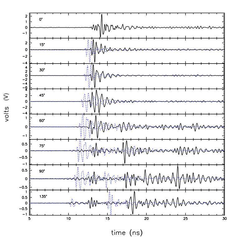
FIG. 7.: Typical traces of horn response versus angle. The pulses from the sand remain in phase as the angle is changed, consistent with power emanating from the center of the target. The angular dependence of the time delay for the empty target is shown for comparison in dotted lines.

There are two obvious distinctions between the traces for full target (solid) and empty target (dotted) in Figure 7. First, the “full” profiles at low angles appear about 0.8 ns later than the corresponding “empty” profiles. This is expected since the refractive index of the sand induces a delay for any radiation that propagates through it, whether it originates at the end of the beampipe or from the center of the target. The index of refraction for silica sand at these frequencies is expected to be in the range of 1.5-1.7 depending on water content; our data indicates a value 1.55 as noted above.

Second, the target-full profiles in general remain centered around 13 ns, rather than showing the progression to earlier times that is evident in the target-empty data. This indicates that the emission in the target-full case arises from near the center of the target, since the horn antenna position was at a fixed radius from this point. The delay of these pulses is also consistent with the geometry.

For example, in the $75^{\circ}$ profile, there is a 2 ns delay of the full-target pulse relative to the empty-target pulse. From Fig. 8, the delay should correspond to the difference between the direct ray path from the beampipe end to the horn (for the empty target case), and the composite path in the full-target case, including: the beam path from beampipe end to the target center, and then from the target center (where the RF emission is formed) to the horn. Thus the delay should be

$$\tau=c^{-1}(A/\beta+nB+C-D)$$ (8)

where $A,B,C,D$ are the distances from the end of the beampipe to the target center, the target center to the target edge, the target edge to the horn face, and the beampipe end to the horn face, respectively.

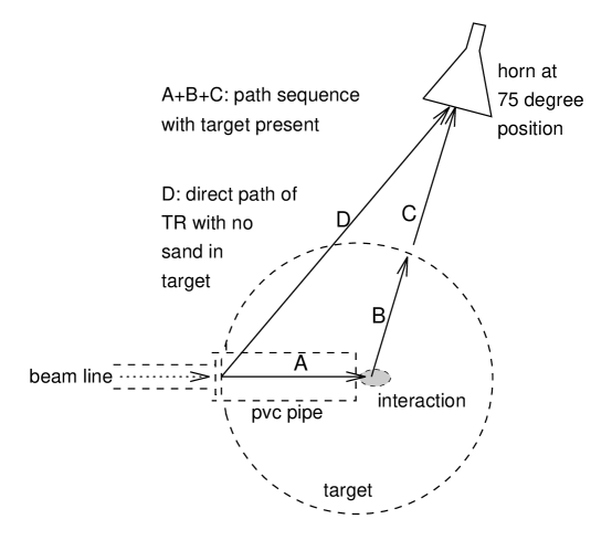
FIG. 8.: An example of the time delay geometry for two different cases: emission from the end of the beampipe directly to the horn, when no sand is present in the target; and the case of the beam first interacting with the target and producing emission radiated from its center to the horn, through the refractive target.

Since $A\simeq 70$ cm, $nB\simeq 1.5\times 40$ cm, $C=55$ cm, and $D=130$ cm, the expected delay is 1.75 ns, consistent with what is observed, within the errors in our knowledge of the target position. Note that the the polyethylene tub and PVC pipe in the case where he target is empty have a negligible effect on the pulse propagation since they have modest microwave dielectric constants, and thicknesses much less than a wavelength.

Based on the timing analysis presented here, we thus identify the time window between 12 and 15 ns as the relevant portion of the plot in which to evaluate the possible presence of a radiation component emanating from the region near the target center. We will focus our attention on the pulse energy in this time window in the sections that follow.

E Target-full angular power distributions

With the target filled, we now expect production of RF emission from the beam dump region. In addition, there is still TR emitted from the beampipe end which now passes through the target, where it is significantly refracted by the cylindrical geometry and the refractive material present. Thus although the target is designed to allow for radial propagation of emission from near its center with minimal effects from refraction; the refraction of emission not originating at the target center will be significant and must be explicitly accounted for.

FIG. 9.: Partial ray trace of the TR from the aluminum foil through the sand target.

Fig. 9 shows the behavior of some of the rays associated with the beampipe end TR, calculated using standard geometrical ray-tracing equations. As the radiation enters the target along the PVC input pipe wall, it is initially refracted away from the beam axis. Upon arriving at the target boundary, however, the large change in the index of refraction from sand to air tends to produce total internal reflection for rays at large angles, and those that do escape tend to be highly forward-beamed. The net result is that none of the TR from the beampipe end can propagate to angles greater than $\sim 50^{\circ}$ with respect to the target center. In fact the transmission coefficient at angles just above the angle of total internal reflection are also quite small, and combining this effect with the forward-peaked nature of the TR from the beampipe, we find that there is virtually no contribution from the beampipe TR beyond the $45^{\circ}$ position.

FIG. 10.: The measured pulse energy (normalized by solid angle) at each angular position for the full target is plotted along with the theoretically expected Cherenkov angular distribution (dashed line); Also plotted is the expected distribution of lensed forward TR (dotted line), based on the ray tracing described in the text.

Fig. 10 shows the measured pulse energy (normalized to unit solid angle) at each of the angular positions around the target-full case. We have also plotted (dashed curve) the expected CR angular spectrum from the target center, using the measured index of refraction of the sand and the predicted length of the electron cascade near target center, taken here to be 4 cm. This curve was scaled down by a factor of 30 to match the lower TR curve in figure 6. We have also plotted an estimate of the angular intensity of the forward-lensed TR (dotted lines). This curve has considerably more uncertainty since it depends on both the accuracy of our ray-tracing, and on theoretical estimates for which the assumed conditions (infinite media and tracklengths) do not apply.

At angles smaller than $\sim 50^{\circ}$, the TR from the beampipe is focussed forward by the target and adds to the CR from the target center. For $50^{\circ}<\theta<\sim 90^{\circ}$, we expect little or no contribution of TR from the beampipe, and we assume forward TR from the quartz window is suppressed since the beam stops well within the formation zone. Thus we expect CR to be the main contribution here. At $\theta\gg 90^{\circ}$, both CR and backward TR from the quartz window contribute, though again the TR undergoes some focusing which tends to backward–beam it. We have not attempted to assess the backward TR in any quantitative way, but note that it is likely to contribute to the increased pulse energy seen at $135^{\circ}$ compared to 90^∘.

It is evident from the plot that we have not yet seen a clear signature of CR at expected levels. In the remainder of this section we present other evidence which, although somewhat indirect, does support the presence of CR emission in our observations, though it does not account for the observed power deficit.

F Coherence at $60^{\circ}$

We are able to assess the coherence properties of the emission observed at $60^{\circ}$ from the target center by investigating the variation of observed power with the intrinsic variation of electron bunch charge within a run. Fig. 11 shows a plot of the logarithm of the integrated power at 60^∘ within this window as a function of the logarithm estimated electron number in the beam pulse. The fitted slope of this distribution is $1.93\pm 0.09$ which is consistent with the emission being primarily coherent. Partial loss of coherence might be expected in this case since the beam must propagate through 50 cm of air path before it enters the target. Note that this plot does not cover as large a range of currents as Figure 5.

FIG. 11.: Detected power plotted as a function of electron number in the beam pulse, for two target-full runs at a horn angle of $60^{\circ}$. A fit to the slope of the ensemble of points is also shown. Perfect coherence would give a slope of 2.0, complete incoherence a slope of 1.0.

The observed level of coherence for these pulse charges is consistent within errors with the overall coherence of the TR measurements presented above, since these measurements were made at beam currents which were at the high end of our range, where we had previously seen a tendency for the coherence to roll off. This observed coherence is of course expected from both TR and CR emission.

G Polarization dependence

In the same way that we expect both CR and TR to be coherent emission processes, they share similar polarization properties as well. In the limit of perfect coherence, we expect both forms of emission to be completely linearly polarized in the plane containing the beam velocity vector and the direction of observation. For our observation geometry this angle corresponds to $0^{\circ}$, or horizontal polarization.

A possible signature of a distinct emission component could be indicated by a significant change in the polarization state of the observed radiation over a particular range of angles. This is due to the fact that at certain angular regions of our measurements, the received radiation is a superposition of TR refracted from the beampipe end (from different ray paths), and possible CR from the target center. Such superposition of components of different phases can be expected to produce noisy polarization measurements with a poorly defined plane of polarization. In contrast, observations over an angular region where one radiation component predominates should have less noise and a more clearly defined plane of polarization. This is in fact what we have observed.

Linear polarization measurements were made for four of the eight angles around the full target. These measurements consisted of recording the pulse profile at three different horn rotations around the axis normal to its receiving aperture. The microwave horn we employed was designed to have a principal E-plane, and had a cross-polarization rejection of $\sim 20$ dB for linear polarization. Thus we can estimate three of the four Stokes parameters $I,Q,U,V$ by making three intensity measurements at $0^{\circ},~{}45^{\circ},~{}90^{\circ}$. Under these conditions, we have:

$$V_{0}^{2}~{}=~{}{1\over 2}(I+Q),~{}V_{45}^{2}~{}=~{}{1\over 2}(I+U),~{}V_{90}^{2}~{}=~{}{1\over 2}(I-Q)$$ (9)

where $V_{0},V_{45},V_{90}$ are the voltage measurements at the specified angles. and these results can then be combined in the usual way to give the fractional polarization $P$, and the polarization angle $\phi$:

$$P~{}=~{}{\sqrt{Q^{2}+U^{2}}\over I};\ \tan\phi~{}=~{}{U\over Q}~{}.$$ (10)

The results for the four positions measured are shown in Fig. 12. The different angle positions around the target are plotted columnwise, and the intensity profile for each case is displayed along the top row, followed by the fractional polarization and the polarization angle along the bottom of the plot. For the fractional polarization and angle, only points with intensities greater than 0.05 of the maximum are plotted; thus each point has relatively high SNR, and the observed scatter is intrinsic rather than statistical. For TR and CR that arise from a single location and are unscattered, we expect the fractional polarization to be $\sim 1$ and the plane of polarization to be horizontal ($0^{\circ}$).

We find that the characteristics of the polarization at angles greater than $50^{\circ}$ are notably different than those of the forward angles where we expect significant superposition of different forward scattered and reflected components of strong TR. At the $0^{\circ}$ position with respect to the target, a somewhat larger scatter in the angle of the plane of polarization is to be expected, due to the effects of being close to the polar axis. In contrast, the $15^{\circ}$ position with respect to the target should give a more clearly defined plane of polarization but also shows a large scatter, consistent with mixing of multiple components in the TR.

FIG. 12.: The normalized power profile in the primary pulse is plotted along the top row, followed by the fractional polarization and the polarization angle, for four positions measured around the target. The fractional polarization and corresponding angle are only plotted where the power is greater than 0.05 of the maximum. The resulting scatter is thus intrinsic, not statistical. The plane of polarization is expected to be $\sim 0^{\circ}$ for direct CR or TR.

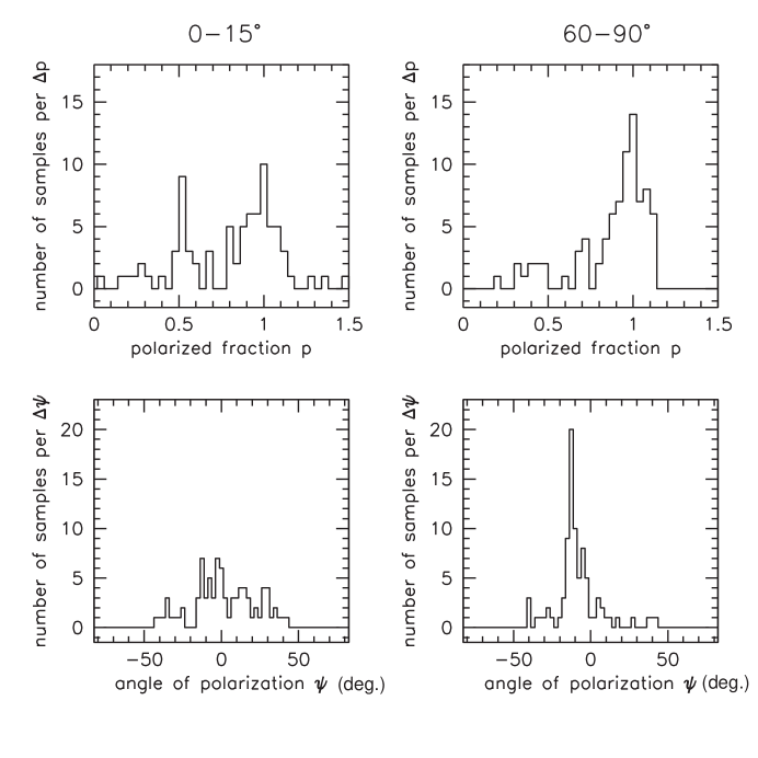
FIG. 13.: Histograms of the sampled fractional polarization and angle of the plane of polarization, for two different angular regions, $0-15^{\circ}$ and $60-90^{\circ}$, showing the distinct behavior for the larger angles, where Cherenkov emission is expected to contribute.

At $60^{\circ}$ we see a markedly different behavior in the plane of polarization, with much less scatter and values that are close to $0^{\circ}$. This behavior is also present but somewhat weaker at $90^{\circ}$. This behavior is displayed more clearly in Fig. 13, where we have now combined the data at the low angles for comparison with the data at the higher angles. It is evident that both the fractional polarization and the plane of polarization are more clearly defined at the larger angles. We interpret this as evidence that we are seeing a single coherent radiation component that displays characteristics consistent with Cherenkov radiation from the target center. We cannot rule out a residual contribution of TR from the beampipe end here, but as we have noted above, at these larger angles we do not expect to see significant TR.

We have also considered the possibility that we are seeing a wide-angle forward TR from the air-quartz-sand interfaces, and little or no CR. Although we cannot rule this out we note that the bulk of the electrons stop well within the formation zone (estimated to be 20-30cm at 60^∘) and we expect that the TR is thus suppressed. In addition, the presence of the sand surrounding the beam (at a radius of $\sim 8$ cm — less than 1 wavelength) as it traverses the target prior to penetrating the quartz window also “smooths” the dielectric transition and will further tend to suppress the TR. We note also that theoretical predictions for the power and angular spectrum of TR for this interface are inconsistent with energy considerations, as we show in appendix A; so we are unable to make reliable estimates of the power that might be present in this case.

V Discussion

In the previous section we have presented results which show a clear signature of coherent transition radiation at GHz radio frequencies from electron bunches. Although this result is not surprising given similar results at far infrared and submillimeter wavelengths, it is to our knowledge the first such demonstration at these longer wavelengths.

In addition, we show evidence consistent with a Cherenkov component in the emission from our target. This evidence relies primarily on the design of the target, which produces an angular window where the TR emission is suppressed, and is strengthened by the presence of distinct, linearly polarized component in the emission near the Cherenkov angle, which contrasts sharply with the TR seen at other angles. However, we do not yet observe either Cherenkov or transition radiation that is consistent with the expected power in our experiment.

One possibility is that complete coherence does not fully obtain in either our TR or CR production, due to possible saturation or self-quenching effects in the electron bunch. There is in fact some evidence that a partial loss of coherence is present in the TR runs (see figure 5). This effect appears to set in only at the highest beam charge values. As discussed in the following subsection such a roll-off for the highest energy showers must happen at some point.

A Implications for cascade radio emission

If we take the value of $N_{e}$ as a measure of the charge excess in a cascade, we can associate our measurements with an equivalent cascade energy $E_{e}\simeq N_{e}/0.2$ GeV, where we have assumed here that the charge excess is 20% of the total charge near shower maximum. For the bunch charges in our experiment, $E_{e}\simeq 5\times 10^{20-21}$ eV, corresponding to energies that equal and exceed the highest energy cosmic ray cascades detected to date.

Zas, Halzen, and Stanev [11] have shown that high energy cascades in solid ice, under the assumption of full coherence, produce a total radio CR pulse energy $W$ which can be written as

$$W~{}\simeq~{}5\times 10^{-15}~{}\left({E_{e}\over 1~{}{\rm TeV}}\right)^{2}\left({\nu_{max}\over 1~{}{\rm GHz}}\right)^{2}~{}~{}{\rm\mu J}~{}$$ (11)

where $\nu_{max}$ is the highest frequency observed (in practice loss of coherence sets in for $\nu_{max}\geq 2$ GHz). This quadratic dependence of radio power implies a saturation energy: that is, we can equate the total energy in equation 11 with the total energy in the shower to derive an upper limit $E_{max}$ for the maximum energy at which this relation can be valid. Thus we find

$$E_{max}~{}=~{}3\times 10^{24}~{}{\rm eV}~{}.$$ (12)

which is only a factor of $600$ above our highest equivalent cascade energy. However, $E_{max}$ represents the value at which all of the shower energy is lost to the RF pulse; in fact a more conservative approach would require some type of equipartition of the shower energy among other energy-loss mechanisms such as ionization, and would require that the radiation reaction of the shower conserve total momentum. Thus we predict that equation 11 must begin to lose validity at some critical energy $E_{crit}=\epsilon E_{max}$, where we expect that $\epsilon\leq 0.1$. Our data in fact suggest $\epsilon\sim 0.001$ if the loss of coherence we observe at the highest bunch charges is due to some related effect.

Similar arguments can be applied directly to the theoretical power expected in our experiment from both CR and TR. If we integrate over just the forward angles for our experimental conditions, the total expected power in our passband is $\simeq 60$ $\mu$J. The total energy per electron bunch is $N_{e}E_{e}\simeq 2.2\times 10^{5}$ $\mu$J for 15 nC and 15.2 MeV electrons. Thus the theory predicts that about 1 part in 3600 of the bunch energy to be radiated in our band for fully coherent emission. However, this implies that only a factor of 60 increase in the bunch charge would lead to a complete loss of energy of the bunch to coherent RF emission. Thus it appears that our experimental condition may be more severely affected by possible loss of coherence than equation 11 implies.

B Lower limits on cascade power at $E_{0}\geq 10^{20}$ eV

In spite of the difficulty in finding a satisfactory resolution to the apparent discrepancies in observed vs. theoretical power, we can still use our observed values to derive lower limits on the expected power from both TR and CR from cascades in materials similar to what we have observed. For TR, refractory materials such as sand, lunar regolith, or ice produce nearly the same spectrum as the aluminum window used on our beampipe end. Thus our results are directly applicable to cascades that encounter interfaces in these materials, for example, a cascade that emerges from the material into either air or vacuum is closely analogous to what we have observed for TR. In the CR case, our results are more uncertain but may still provide a preliminary experimental lower limit in estimating cascade emission.

1 Transition radiation

The highest values in our TR measurements of the pulse energy were $\sim 6$ $\mu$J sr^-1. Converting these to the flux density units commonly used in radio astronomical measurements, we estimate that the TR flux density produced at earth from a cascade of $E_{0}=5\times 10^{21}$ eV emerging from the surface of the lunar regolith is

$$S(\theta\simeq 10^{\circ})~{}\geq~{}5000\left({E_{0}\over 5\times 10^{21}~{}{\rm eV}}\right)^{1.9}~{}{\rm Jy}$$ (13)

where $1$ Jy $\equiv 10^{-26}$ W m^-2 Hz^-1. Since the TR angular distribution appears to be confirmed by our data for these conditions, we can also estimate that the maximum flux density for this case, at an angle of $\sim 1.5^{\circ}$ from the cascade axis, is about a factor of 20 higher than at $\sim 10^{\circ}$:

$$S_{max}(\theta\simeq 1.5^{\circ})~{}\geq~{}10^{5}\left({E_{0}\over 5\times 10^{21}~{}{\rm eV}}\right)^{1.9}~{}{\rm Jy}~{}.$$ (14)

The large antennas used in lunar pulse searches have demonstrated the ability to achieve noise levels of order 400 Jy [10] or less. Thus it appears that the energy threshold for detection of events by TR alone is $5\times 10^{20}$ eV. Here we have not considered the indications of higher measured pulse energy given by our dipole measurements. If these results are correct, the energy threshold may be an order of magnitude lower.

These results support the claim [14] that TR detection of cascades is feasible for the case that a cascade emerges through some surface into a medium transparent to radio emission, and this analysis also applies to detection of cascades on earth. For example, our measurements could be applied to the case of a shower that was initiated in air and then entered ice near a subsurface radio array, such as has been proposed and prototyped in Antarctica [3, 5, 4]. In this case, we can write the threshold energy more generally as

$$E_{thr}^{TR}~{}\leq~{}5\times 10^{20}\left({\Delta\nu\over 900~{}{\rm MHz}}\right)^{-1/2}\left({A_{eff}\over 2500~{}{\rm m^{2}}}\right)^{-1/2}\left({R\over 3.8\times 10^{8}~{}{\rm m}}\right)\left({T_{sys}\over 220~{}{\rm K}}\right)^{1/2}~{}{\rm eV}.$$ (15)

where $A_{eff}$ is the total effective collecting area of the antenna or antenna array (including aperture efficiency), $R$ is the distance to the cascade, and $T_{sys}$ the system temperature. Here we have assumed that full coherence obtains at lower cascade energies; thus the exponent for the energy term above was assumed to be 2.0 rather than 1.9 as we have used at the highest energies.

If we apply this equation to the case of an antenna array in ice comprising 10 m² effective aperture, operating at $T_{sys}$ of 1000 K with a 900 MHz effective bandwidth, the system will have a TR detection capability for cascades with $E_{0}\simeq 2\times 10^{16}$ eV entering the ice from above, out to a distance of 250 m. However, we caution that formation zone effects may be important depending on how rapidly the near-surface refractivity of the ice changes with depth.

2 Cherenkov radiation

Although we attempted to optimize our experiment in favor or CR detection rather than TR, we cannot yet claim to have yet made measurements of it adequate to allow us to make definite statements about the application of these data to the detection of radio CR from high energy cascades. One thing is much more clear to us after having performed this initial experiment than was evident in the literature: the processes that produce these two forms of radiation are physically very closely aligned.

The problem of separating the two forms of emission is particularly acute when the radiation can be formed in nearly the same physical location, such as at the quartz window entering the target in our case. In fact, the theoretical formulations for TR at this point do not themselves clearly separate the two processes; as we noted in an earlier section, “Cherenkov-like” components appear even in the TR equations. Thus, we suggest that a more complete theoretical basis for TR formation under realistic conditions with finite track lengths and boundaries be developed.

An important aspect of the operating regime of our experiment is that the detected Cherenkov power should scale quadratically with both the total track length as well as the number of particles. For solid materials, the mean electron energy near shower maximum for a typical high energy cascade is closer to $\sim 100$ MeV rather than the 15 MeV used in our experiment. Thus the total track length is much longer and the Cherenkov production is more directive and therefore more intense near its peak angle. Any scaling from experiments similar to ours must account for this effect.

If we do attribute the observed power of 0.014 $\mu$J sr^-1 at our $60^{\circ}$ angle primarily to Cherenkov radiation, we can make a tentative estimate of the possible energy threshold for CR detection. A cascade of energy $\sim 10^{20}$ eV in ice or the lunar regolith will have a length of order 10 m[11] near shower maximum. For this length, the implied angular enhancement in the intensity is of order $10^{4}$, giving $\sim 140~{}\mu$J sr^-1, comparable to the observed TR intensity at an angle of $\sim 1.5^{\circ}$. The implied cascade energy threshold, using the same arguments as above, is therefore comparable to that implied by our TR results. For the lunar regolith, $E_{thr}~{}\approx~{}5\times 10^{20}$ eV, similar to values estimated from complete electromagnetic simulations of ultra-high energy cascades [11, 6, 12]. If our assumptions are correct, this value is conservative, and we expect further experiments to yield a potentially much lower cascade energy threshold for coherent Cherenkov detection.

C Implications of RF lensing effects

In concluding this section we note that the lensing effects on the forward-beamed TR emission that we have observed in our target-full configuration have potentially important implications for experiments to detect cascade emission from the lunar regolith or other materials observed through a refractive interface. Under these conditions, our results suggest that total internal reflection of the cascade radio emission can strongly suppress it at certain angles and under certain geometrical configurations.

This effect is potentially helpful in distinguishing particles such as hadronic cosmic rays or photons (which interact immediately upon entering the refractive material) from neutrinos (which can interact near the surface of the material after traversing it over large distances). In the latter case, since the critical angle for total internal reflection is the complement of the Cherenkov angle at a vacuum interface, the CR can exit the surface into the vacuum. However, in the former case, the CR from the cascade will suffer total-internal reflectance and will not emerge from the surface. Clearly, surface irregularities at scales approaching an RF wavelength will modify this conclusion at some level, but to first order this effect will tend to suppress the detection of cosmic ray events relative to upcoming neutrino cascades in lunar observations.

VI Future work

Our ability to separate TR from CR in this analysis depended on the geometry and precise timing. TR from the vacuum window was lensed into most of our observing angles. In a new experiment, with the window further forward, much of this effect will be avoided. In addition, taking more position angles with full polarization measurements will further assist us in separating prompt from lensed power.

Our results suffer in part from the difficulty of achieving accurate power calibration. In future work, we will significantly improve our power calibration capabilities. We would also plan to more carefully calibrate the beam current measurements with a Faraday cup to determine if the apparent loss of coherence that we see at high beam currents is real or due to nonlinearities in our measurement.

Future experiments along these lines should also be done using pulsed high energy photons, whose radiation length in sand (30–40 g cm^-2) will allow the shower to develop within the target and will thus avoid the generation of transition radiation at the beampipe end and entrance to the target.

On the theoretical side, analytic or parametric formulas for dealing with disturbances of the charge inside the TR formation zone would be helpful. We would also like to see a theoretical understanding of the critical energy beyond which the coherence fails to scale at $N_{e}^{2}$ which must be important near the energies and currents we are using.

A Predictions for radio-frequency coherent TR

To illustrate some of the complexity in evaluating the theoretical predictions for TR in the radio frequency regime, we have calculated the forward angular spectra for TR in a number of configurations relevant to our experiment, using equation 1. We have chosen a frequency range of 1.7–2.6 GHz, corresponding to the range used in our experiment. We have considered emission from a single bunch of 15 MeV electrons with a total charge of 15 nC. For our purposes here we have scaled the results by a factor of $N_{e}^{2}$, corresponding to perfect coherence.

Figure 14 shows the results of this analysis for several combinations of upstream and downstream materials, noted in the panel text. In each case we have plotted the angular spectrum predicted by equation 1 with a solid line. Also plotted (dashed curve) is the integral over the angles shown of the total energy of the pulse. The dotted curve shows the total available kinetic energy of the electron bunch.

In Fig. 14a we plot predictions for the case most commonly encountered in the experimental literature for submillimeter and far-IR measurements of TR from electron bunches: radiation from the exit of the bunch through a beampipe metal window into air. In this case TR is forward-peaked at an angle of $\sim 1/\gamma$, and the total energy radiated in coherent TR in this case is $\sim 2\times 10^{-4}$ of the available kinetic energy. As we have seen above, we find that our data confirms the angular distribution shown here, though not the total pulse energy.

In Fig.14b, we plot the prediction for the case of the electron bunches exiting a metal window directly into a dielectric material with $n=1.5$ corresponding to silica sand as we have used in our experiment. Here the strong peak at the nominal Cherenkov angle is evident, and the forward peak seen in the previous pane is no longer present. Also important is the fact that the total energy in the coherent emission now approaches 10% of the available kinetic energy. This prediction thus appears to be physically improbable.

In Figs. 14c and d we see even more complex behavior in the cases of a sand-to-air and air-to-sand transitions. Clearly in both cases the predicted total energy exceeds the available kinetic energy and thus the theory appears to be inadequate in treating this combination of parameters.

This example highlights two issues that we have faced in this experiment: First, what is the actual TR angular distribution in cases that differ from the simple metal-to-air interface commonly treated by the theory? Second, how do we resolve the issue of what fraction of the total energy in a particle bunch can reasonably be emitted into coherent radiation?

FIG. 14.: Predictions from equation 1 for emission of coherent radio frequency TR using various dielectric combinations. The wavelength range used in 11-18 cm, and the electron bunches have an energy of 15 MeV with a bunch charge of 15 nC. In each case the solid curve gives the angular spectrum, the dashed curve the integral of that spectrum, and the dotted curve the total available kinetic energy of the bunch. (a) The metal-to-air interface. (b) The aluminum-to-sand interface predicts a Cherenkov-like distribution which appears to emit too large a fraction ($\sim 10$%) of the total energy into TR. (c& d). The sand-air and air-sand interfaces predict a complex behavior which is physically unrealistic since the total energy exceeds that of the available kinetic energy.

REFERENCES

- [1] G. A. Askaryan, Zh. Eksp. Teor. Fiz. 41, 616 (1961) [Soviet Physics JETP 14, 441 (1962)]; G. A. Askaryan, Zh. Eksp. Teor. Fiz. 48, 988 (1965) [Soviet Physics JETP 21, 658 (1965)].
- [2] I. N. Boldyrev et al., 3rd Intl. Work. on Neutrino Telescopes, M. Baldo-Ceolin (ed.), Venice, 1991.
- [3] G. M. Frichter, J. P. Ralston, and D. W. McKay, Phys. Rev. D. 53, 1684 (1996).
- [4] D. Seckel et al., Proc. 26th. Intl. Cosmic Rays Conf., (1999).
- [5] D. Besson et al., Proc. 26th. Intl. Cosmic Ray Conf., (1999).
- [6] J. Alvarez–Muñiz and E. Zas Proc. 25th Intl. Conf. on Cosmic Rays, ed. M.S. Potgeiter et al. vol. 7, 309 (1996).
- [7] T. H. Hankins, R. D. Ekers, and J. D. O’Sullivan, MNRAS 283, 1027 (1996).
- [8] I. M. Zheleznykh, Proc. 13th Intl. Conf. on Neutrino Physics and Astrophysics (“Neutrino 88”), World Scientific, Boston, ed. J. Schreps, p. 528 (1988).
- [9] R. D. Dagkesamanskii, and I. M. Zheleznykh, Zh. Eksp. Teor. Fiz. 50 233 (1989) [JETP Lett., 50 259 (1989)].
- [10] P. W. Gorham, K. M. Liewer, and C. J. Naudet, Proc. 26th Intl. Cosmic Ray Conf., v 2, 479, (1999); also astro-ph/9906504.
- [11] E. Zas, F. Halzen, and T. Stanev, Phys. Rev. D 45, 362 (1992).
- [12] J. Alvarez–Muñiz and E. Zas, Phys. Lett. B, 411, 218 (1997).
- [13] J. Alvarez–Muñiz and E. Zas, Phys.Lett. B, 434, 396, (1998).
- [14] Markov, M. A., and Zheleznykh, I. M., Nucl. Instr. Meth. A248, 242, (1986).
- [15] J. R. Neighbors, F. R. Buskirk, and A. Saglam, Phys. Rev. A, 29, 3246 (1984).
- [16] X. K. Maruyama et al., J. Appl. Phys. 60, 518 (1986).
- [17] T. Nakazato, et al., Phys. Rev. Lett. 63, 1245 (1989).
- [18] Y. Shibata, et al., Phys. Rev. A 44, 3449 (1991).
- [19] K. Ishi, Y. Shibata, T. Takahashi, H. Mishiro, T. Ohsaka, M. Ikezawa, Y. Kondo, T. Nakazato, S. Urasawa, N. Niimura, R. Kato, Y. Shibasaki, and M. Oyamada, Phys. Rev. A, 43, 5597 (1991).
- [20] T. Takahashi et al., Phys. Rev. E 50, 4041 (1994).
- [21] Y. Shibata et al., Phys. Rev. E 49, 785 (1994).
- [22] V. L. Ginzburg and V. N. Tsytovich, Transition Radiation and Transition Scattering, (New York: Adam Hilger Press), 1990.
- [23] G. M. Garibian, Zh. Eksp. Teor. Fiz. 33, 1403 (1957) [Soviet Physics JETP 6, 1079 (1958)]; G. M. Garibian, Zh. Eksp. Teor. Fiz. 37, 527 (1960) [Soviet Physics JETP 10, 372 (1960)].
- [24] L. Warski et al., J. App. Phys. 46, 3644 (1975).
- [25] I. E. Tamm, J. Phys. (Moscow) 1, 439, 1939.
- [26] L. A. Vardanyan, G. M., Garibyan, and C. Yang, Izv. Acad. Nauk. Arm. SSR Fiz. 10, 350 (1975).
- [27] Conde, M. E., et al. Phys. Rev. ST Accel. Beams 1, 041302.
- [28] A. R. Von Hippel, ed., Dielectric Materials and Applications, (Artech House Publishers), 1995.
- [29] SLAC publication SLAC-265, W. Nelson et al. December 1985.
- [30] E. V. Jull, Aperture Antennas and Diffraction Theory, (New York: Peter Peregrinus Ltd.) 1981, see chapter 5.