Abstract

We consider a wave-function approach to the false vacuum decay with gravity and present a new method to calculate the tunneling amplitude under the WKB approximation. The result agrees with the one obtained by the Euclidean path-integral method, but gives a much clearer interpretation of an instanton (Euclidean bounce solution) that dominates the path integral. In particular, our method is fully capable of dealing with the case of a thick wall with the radius of the bubble comparable to the radius of the instanton, thus surpassing the path-integral method whose use can be justified only in the thin-wall and small bubble radius limit. The calculation is done by matching two WKB wave functions, one with the final state and another with the initial state, with the wave function in the region where the scale factor of the metric is sufficiently small compared with the inverse of the typical energy scale of the field potential at the tunneling. The relation of the boundary condition on our wave function for the false vacuum decay with Hartle-Hawking’s no-boundary boundary condition and Vilenkin’s tunneling boundary condition on the wave function of the universe is also discussed.

I Introduction

In the previous literature, the false vacuum decay with gravity was investigated, in essence, by a naive extrapolation of well-established methods used for the Minkowski background[1]. There are two methods to calculate the decay rate of false vacuum, one using the Euclidean path integral and the other constructing a WKB wave function. However, in both approaches such extrapolation is valid only for a tunneling potential $V(\phi)$ satisfying the thin-wall condition (we shall come back to this point below).

The false vacuum decay in quantum field theory on the Minkowski background is analyzed in the semiclassical way (i.e., in the WKB approximation) as follows[2]. First, the Euclidean classical equation of motion for the field $\phi$ (we consider a real scalar field throughout the paper) is solved by assuming the $O(4)$ symmetry on the field configuration with the boundary condition that the solution is regular at the origin and asymptotically approaches the false vacuum at infinite radius. There will be two such solutions; one trivially sitting at the false vacuum and the other that leaves the origin from a field value near the true vacuum and goes over the potential barrier. We call the former the false vacuum instanton and the latter the bounce instanton. We can take either the path-integral approach or the wave-function approach.

In the path-integral approach, we sum up the contribution of instantons and fluctuations around them to obtain the tunneling amplitude or the decay rate of false vacuum. If we denote the Euclidean action of the false vacuum instanton by $S_{F}$ and that of the bounce instanton by $S_{B}$, the decay rate is given by $\Gamma\sim e^{-(S_{B}-S_{F})}$. In passing, we note that in the Minkowski background it is customary to set $V(\phi_{F})=0$ so that $S_{F}=0$. But one can take a different choice, $V(\phi_{F})\neq 0$, in which case both $S_{F}$ and $S_{B}$ would diverge but the difference is well-defined and independent of the value of $V(\phi_{F})$.

In the wave-function approach, we construct a one-parameter family of 3-dimensional field configurations from the everywhere-false-vacuum configuration to the configuration with the true vacuum bubble about to expand in the false vacuum sea (the critical bubble configuration). Then, exponentiating the action of these configurations we obtain the WKB wave function(al) describing the tunneling of the field from the false vacuum state to the state of the critical bubble [3]. Then the tunneling amplitude is obtained by taking the square of the ratio of the final state wave function to the initial state wave function, which is also given by $e^{-(S_{B}-S_{F})}$.

Since these two different approaches give the same result, and since there is one-to-one correspondence between a classical solution and a WKB wave function, we may justify the interpretation of the bounce instanton as describing the tunneling process and its analytic continuation to the Lorentzian space-time as describing the classical configuration of the field after false vacuum decay.

A trouble arises when one attempts to extrapolate the above procedure to the case of false vacuum decay with gravity. First, the scalar field equation is now coupled with the Friedmann equation that governs the scale factor of the $O(4)$ symmetric metric. Second, and most problematically, the 4-dimensional Euclidean space becomes inevitably compact with topology of $S^{4}$ when gravity is taken into account (we assume $V(\phi_{F})>0$ where $\phi_{F}$ is the field value at the false vacuum and a potential of the shape depicted in Fig. 1), i.e., not $\mbox{${\rm I\!R}$}^{4}$ as in the case of flat space-time. Of course a bounce solution still exists in the presence of gravity, first obtained by Coleman and DeLuccia[1]. However, there will be no bounce solution that admits a 3-dimensional slice on which the field is asymptotically at false vacuum everywhere; an instanton leaving, say, the north pole of $S^{4}$ from the true vacuum side does not reach the false vacuum when arriving even at the south pole. Furthermore, the standard dilute gas approximation to obtain the decay rate in the path-integral approach, in which the 4-volume occupied by a vacuum bubble is assumed to be negligible compared with the whole Euclidean 4-volume, fails.

Nevertheless, there is one special case in which the extrapolation can be almost justified. It is the thin-wall limit[5]. In this case, the field $\phi$, which is sitting on the true vacuum side of the barrier at the north pole, varies abruptly at the position of the bubble wall sharply located in the northern hemisphere and $\phi=\phi_{F}$ everywhere outside the bubble. Then, the solution admits a maximal 3-surface on which the extrinsic curvature of the 3-surface vanishes and $\phi=\phi_{F}$ everywhere. Through this surface, we can analytically continue to the Lorentzian solution that describes the false vacuum state. The critical bubble configuration that describes the moment of bubble nucleation is also a maximal 3-surface, and analytic continuation through the surface gives the space-time with an expanding bubble. Thus we obtain a one-parameter family of 3-dimensional configurations that interpolates between the false vacuum and critical bubble configurations.

However, only a very restricted class of potentials admits bounce instantons in the thin-wall limit. Namely, the ratio of the mass scale $m$ of the curvature at the top of the potential barrier, $m^{2}=-d^{2}V/d\phi^{2}(\phi_{top})$, to the typical mass scale $M$ of the potential energy density must be very large (rigorously speaking, it must be infinitely large in the exact thin-wall limit). In other words, the barrier must be extremely sharply peaked. We note that this is somewhat different from the definition of the thin-wall limit originally discussed by Coleman and DeLuccia[1]. In our definition, since the Euclidean 4-volume is proportional to $(GM^{4})^{-2}$ while the 4-volume of a bubble is $O(m^{-4})$, the thin-wall limit implies small bubble radius, provided $M$ is smaller than the Planck scale, i.e., $GM^{2}<1$. Field potentials with such a feature are apparently not general. However, previous discussions on the false vacuum decay with gravity have been relied on the picture of a bounce instanton having the feature of the thin-wall limit. For example, it is widely believed that the formula $\Gamma\sim e^{-(S_{B}-S_{F})}$ is still valid even when the bounce solution does not have the thin-wall feature at all. Furthermore, the interpretation of such a bounce as describing the tunneling process and describing the classical evolution from the critical bubble state has been adopted without serious considerations.

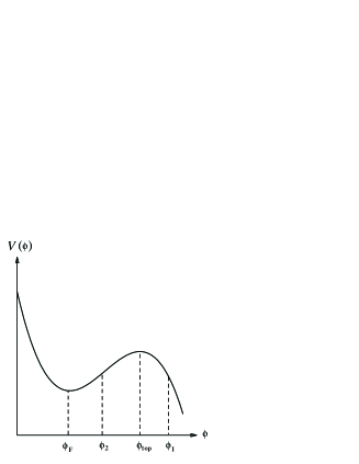
FIG. 1.: A schematic picture of the potential $V(\phi)$ of a scalar field discussed in the text.

In this paper, we propose a new method to calculate the wave function describing false vacuum decay with gravity, which is not restricted to the thin-wall limit. Our method gives a picture of tunneling substantially different from that in the Minkowski background, but nevertheless our wave function interpolates between the false vacuum state, which is described by the trivial instanton sitting at false vacuum, and the state at the bubble nucleation, which is a maximal 3-slice containing the critical bubble of the bounce solution.

The paper is organized as follows. In Section II, we first review the mini-superspace Wheeler-DeWitt equation for $O(4)$ symmetric configurations and the WKB approximation. Then we describe our method. We construct a one-parameter family of spatial configurations that interpolates between the false vacuum state and the critical bubble state. As we are interested in the WKB approximation, we consider a classical path connecting these two states. As pointed out in the above, no ‘single’ classical solution admits such a path. However, a unique feature of false vacuum decay with gravity is that one can match the ‘two’ instantons (the false vacuum instanton and the bounce instanton) smoothly across the ‘south pole’ of each instanton. In section III, by solving the Wheeler-DeWitt equation we explicitly perform this matching and construct the wave function that contains both the false vacuum and critical bubble states, hence describes the false vacuum decay with gravity for a wide class of tunneling potentials. It is then straightforward to calculate the tunneling amplitude. The result recovers the Minkowski result if we take the zero-gravity limit $G\to 0$, and also agrees with the decay rate obtained in the path-integral method with a naive extrapolation of the formula, $\Gamma\sim e^{-(S_{B}-S_{F})}$. Our result supports the standard interpretation that the bounce solution, despite the fact it does not contain the false vacuum configuration at all, does describe the classical evolution after false vacuum decay by analytic continuation through the critical bubble configuration. Section IV is devoted to discussions. A covariant formulation of the WKB wave function for tunneling is recapitulated in Appendix A.

In the rest of the paper, we keep $\hbar$ and $G$ explicit to clarify the WKB order as well as the effect of gravity.

II Formulation

In this section, we describe our method to construct a relevant classical path in the Euclidean regime that determines the WKB tunneling wave function.

A Instantons and WKB approximation

We consider the action,

$$S=\int d^{4}x\sqrt{g}\left[\frac{{\cal R}}{24\pi^{2}\kappa}-\frac{1}{2}g^{\mu\nu}\partial_{\mu}\phi\partial_{\nu}\phi-V(\phi)\right],$$ (1)

where $\kappa:=2G/3\pi$, and the potential $V(\phi)$ as illustrated in Fig. 1. We confine our attention to WKB wave functions that are described by classical solutions having $O(4)$ symmetry. Hence we consider the metric in the form,

$$ds^{2}=-N^{2}(t)dt^{2}+a^{2}(t)d\Omega^{2}_{(3)}$$ (2)

in which $d\Omega^{2}_{(3)}$ is the metric on a unit 3-sphere, and $\phi=\phi(t)$. In this case the action in the first-order form becomes

$$S=\int dtL\,;\quad L=P_{a}\dot{a}+P_{\phi}\dot{\phi}-{\kappa N\over 2a}\left(-P_{a}^{2}+{1\over(2\pi^{2}\kappa)a^{2}}P_{\phi}^{2}-{a^{2}\over\kappa^{2}}Q(a,\phi)\right).$$ (3)

Then the Wheeler-DeWitt equation is written down as

$${\kappa\over{2a}}\left[\hbar^{2}\frac{\partial^{2}}{\partial a^{2}}+\hbar^{2}{p\over a}{\partial\over\partial a}-\frac{1}{(2\pi^{2}\kappa)\,a^{2}}\hbar^{2}\frac{\partial^{2}}{\partial\phi^{2}}-\frac{a^{2}}{\kappa^{2}}Q(a,\phi)\right]\Psi=0,$$ (4)

where

$$Q(a,\phi)=1-(4\pi^{2}\kappa)\,a^{2}V(\phi),$$ (5)

and $p$ is an arbitrary constant that determines the operator-ordering; $p=1$ corresponds to making the ordering covariant with respect to the superspace metric (see Appendix A).

It should be noted, however, that it is not always necessary to take the $t=$const. 3-geometry as the argument of the wave function. In fact, the critical bubble configuration that describes the moment of bubble nucleation does not respect the $O(4)$ symmetry. Nevertheless, we shall see below that the tunneling amplitude can be calculated solely with the knowledge of the wave function for $O(4)$ symmetric 3-geometries.

The construction of a WKB wave function describing multi-dimensional quantum tunneling was discussed much in the literature [3] and reformulated in a covariant manner in [4]. Given a one-parameter family of configurations that satisfies the Euclidean equations of motion, the WKB wave function along the family can be obtained with this method, as recapitulated in Appendix A. Following this method, we first express the wave function in the form,

$$\Psi=\exp[-W_{0}(a,\phi)/\hbar-W_{1}(a,\phi)+\cdots].$$ (6)

Then at the lowest WKB order, we have

$$\left\{\frac{\kappa}{a}\left(\frac{\partial W_{0}}{\partial a}\right)^{2}-\frac{1}{2\pi^{2}a^{3}}\left(\frac{\partial W_{0}}{\partial\phi}\right)^{2}\right\}-\frac{a}{\kappa}Q(a,\phi)=0,$$ (7)

which is, of course, free from the operator-ordering ambiguity.

Introducing a parameter $\tau$ such that

$$\frac{da(\tau)}{d\tau}:=-\frac{\kappa}{a}\frac{\partial W_{0}}{\partial a}\hskip 21.52771pt\mbox{and}\hskip 21.52771pt\frac{d\phi(\tau)}{d\tau}=:\frac{1}{2\pi^{2}a^{3}}\frac{\partial W_{0}}{\partial\phi},$$ (8)

we find

$${d\over d\tau}\,W_{0}\left(a,\phi\right)=-{a\over\kappa}\,Q\left(a,\phi\right).$$ (9)

The Euclidean equations of motion for $O(4)$ symmetric configurations, $(a(\tau),\phi(\tau))$, with the choice of the lapse $N=1$ are obtained from Eqs. (7), (8) and (9) as

$$\dot{a}^{2}-(2\pi^{2}\kappa)a^{2}\dot{\phi}^{2}-Q(a,\phi)=0\,,$$ (10)

$$\ddot{\phi}+3\frac{\dot{a}}{a}\dot{\phi}=\frac{dV}{d\phi}\,,$$ (11)

$$a\ddot{a}+2\dot{a}^{2}+1=3Q(a,\phi).$$ (12)

The first equation is the (Euclidean) Friedmann equation that corresponds to the energy integral of the remaining two equations. The regularity of the solution requires $\dot{\phi}=0$ at $a=0$.

Equation (9) readily gives the relative amplitudes of the leading-order WKB wave function at two different configurations at $\tau=\tau_{1}$ and $\tau_{2}$,

$$\Psi(\tau_{2})=\exp\left[-W_{0}(\tau_{2};\tau_{1})\right]\Psi(\tau_{1})\,;\quad W_{0}(\tau_{2};\tau_{1})=-{1\over\kappa}\int^{\tau_{2}}_{\tau_{1}}d\tau^{\prime}\,a(\tau^{\prime})Q\left(a(\tau^{\prime}),\phi(\tau^{\prime})\right).$$ (13)

As is well-known, $W_{0}(\tau_{2};\tau_{1})$ is just the Euclidean action integral of the system from the configuration at $\tau_{1}$ to that at $\tau_{2}$.

The solutions relevant to our discussion are the trivial solution sitting at the false vacuum and the bounce instanton. The trivial instanton is explicitly given by

$$\left(a^{FV}(\tau),\phi^{FV}(\tau)\right)=\left(H_{F}^{-1}\sin(H_{F}\tau),\phi_{F}\right)\,;\quad\tau\in[0,\pi/H_{F}],$$ (14)

where $H_{F}=2\pi\sqrt{\kappa V(\phi_{F})}$. It represents a Euclidean 4-sphere of radius $H_{F}^{-1}$ and we call it the false vacuum (FV) instanton hereafter. The bounce instanton is known as the Coleman-DeLuccia (CD) instanton [1, 5]. We denote it by $\left(a^{CD}(\tau),\phi^{CD}(\tau)\right)$ with $\tau\in[\tau_{1},\tau_{2}]$. It also has the topology of $S^{4}$ but the field $\phi$ varies monotonically over the potential barrier as the scale factor $a$ varies from zero to a maximum, then to zero. For later convenience, we set $\left(a^{CD}(\tau_{1}),\phi^{CD}(\tau_{1})\right)=\left(0,\phi_{1}\right)$ where $\phi_{1}$ is on the true vacuum side of the barrier, and $\left(a^{CD}(\tau_{2}),\phi^{CD}(\tau_{2})\right)=\left(0,\phi_{2}\right)$ where $\phi_{2}$ is on the false vacuum side of the barrier. See Fig. 1. The FV and CD instantons embedded in $\mbox{${\rm I\!R}$}^{5}$ are schematically shown in Fig. 2 with 2-dimensions suppressed.

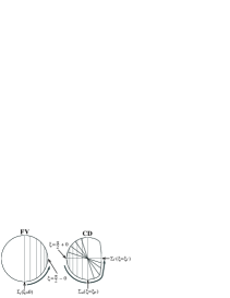
FIG. 2.: Schematic pictures of the false vacuum (FV) instanton and the Coleman-DeLuccia (CD) instanton with 2-dimensions suppressed. The arrow indicates the direction of the increase in the parameter $\xi$ defined in the text.

B One-parameter family of tunneling configurations

As we noted in Introduction, the CD instanton itself does not admit a maximal 3-surface on which $\phi=\phi_{F}$ everywhere, unless the potential satisfies the thin-wall condition. Hence the CD instanton alone cannot describe the tunneling wave function. It is then natural to suppose that the FV instanton plays a role as well. In fact, there is already a hint in the formula for the decay rate, $\Gamma\sim e^{-(S_{B}-S_{F})/\hbar}$, valid in the thin-wall limit, where the action of the FV instanton comes into play.

We therefore consider a possibility to construct a one-parameter family of spatial configurations that connect the false vacuum state and the critical bubble state by matching these two instantons somehow. To look for this possibility, we have to keep in mind that the WKB approximation requires us that such a path should satisfy the classical equations of motion almost everywhere. But this is the crucial point; it is so not everywhere but almost everywhere. In any calculation of a wave function under the WKB approximation, there can be configurations of measure zero that violate the WKB condition, such as turning points of a classical solution, but their existence does not invalidate the calculation if one appropriately performs the matching, e.g., by the method of asymptotic matching. Then we realize that the two instantons may be actually matched through the point $a=0$ where the 3-geometry ceases to exist, hence can be regarded as a turning point of the classical solutions.

With the above considerations in mind, we combine and re-organize the $O(4)$ symmetric families of configurations of the two instantons discussed in the previous subsection to a one-parameter family of configurations which adequately describes the false vacuum decay. We denote this one-parameter family by $(\bar{h}_{ij}(x^{i};\xi),\bar{\phi}(x^{i};\xi))$ where $\xi$ is a non-dimensional parameter. The parameter $\xi$ is assumed to run through a range $[0,\xi_{f}]$ with the initial ($\xi=0$) and final ($\xi=\xi_{f}$) configurations given by the the maximal 3-slice of the FV instanton and the critical bubble configuration of the CD instanton, respectively.

The initial configuration, denoted by $\Sigma_{i}$ in Fig. 2, is given by $H_{F}\tau=\pi/2$ of Eq. (14). We thus set $\xi=H_{F}\tau-\pi/2$ until the scale factor $a$ vanishes,

$$\left(\bar{h}_{ij}(x^{i};\xi),\bar{\phi}(x^{i};\xi)\right)=\left(H_{F}^{-2}\sin^{2}(\xi+\frac{\pi}{2})d\Omega_{(3)}^{2},\phi_{F}\right);\quad\xi\in[0,{\pi/2}).$$ (15)

We match $a=0$ of the above to the point $\left(a^{CD},\phi^{CD}\right)=(0,\phi_{2})$ of the CD instanton, where $\phi_{2}$ is the field value at the ‘south pole’, see Figs. 1 and 2. Note that the values of $\phi$ are different at these two points where the WKB breaks down. However, as we shall see in the next section, this will not be an obstacle since the wave function will be independent of $\phi$ in the vicinity of $a=0$.

For $\xi>\pi/2$, we take the $O(4)$ symmetric configurations of the CD instanton up to the slice $\Sigma_{m}$ shown in Fig. 2, where $\Sigma_{m}$ is the $O(4)$ symmetric slice at $\dot{a}^{CD}=0$ where the 3-volume is maximum, which we denote by $(\bar{h}_{ij},\bar{\phi})=(H_{m}^{-2}d\Omega^{2}_{(3)},\phi_{m})$. Thus

$$\left(\bar{h}_{ij}(x^{i};\xi),\bar{\phi}(x^{i};\xi)\right)=\left(a^{CD}(\xi)d\Omega_{(3)}^{2},\phi^{CD}(\xi)\right);\quad\xi\in({\pi\over 2},\xi_{m}],$$ (16)

where

$$\left(a^{CD}({\pi/2}),\phi^{CD}({\pi/2})\right)=(0,\phi_{2}),\quad\left(a^{CD}(\xi_{m}),\phi^{CD}(\xi_{m})\right)=(H_{m}^{-1},\phi_{m}).$$ (17)

For $\xi>\xi_{m}$, we slice the CD instanton in such a way that all of the configurations contain the common 2-sphere the slice $\Sigma_{m}$ and the final slice $\Sigma_{f}$ of the critical bubble configuration intersect. These slices do not respect the $O(4)$ symmetry but are analogous to the static slices of the de Sitter space of radius $H^{-1}$:

$$h_{ij}(x^{i})=\frac{dr^{2}}{1-H^{2}r^{2}}+r^{2}d\Omega^{2}_{(2)}\,.$$ (18)

As mentioned above, we label the final configuration by $\xi=\xi_{f}$. Thus

$$\left(\bar{h}_{ij}(\xi_{f}),\bar{\phi}(\xi_{f})\right)=(\hbox{the critical bubble 3-geometry}).$$ (19)

As it is clear from the above construction, the lapse function $N$ vanishes at $\Sigma_{m}$, and the geometry is degenerate there. However, this will not be a problem since we have started from the Wheeler-DeWitt equation (4), in which the dynamical variables are $(h_{ij}(x^{i}),\phi(x^{i}))$ of a 3-geometry. Hence, although the lapse function plays a role when a Euclidean classical solution is considered, the vanishing of it is irrelevant to our discussion (in this connection, see [7]). Furthermore, as the relative magnitude of the WKB wave function at two different configuration is simply determined by the action integral between them, and it is independent of deformation of a path between them (as long as the path lies on the space of the classical solution that dominates the wave function), the contribution from the upper-left quadrant of the CD instanton in Fig. 2 swept both by the configurations between $\xi\in(\pi/2,\xi_{m}]$ and $\xi\in[\xi_{m},\xi_{f}]$ cancel each other and only the action of the lower hemisphere determines the relative magnitude of the wave function at $\xi=\pi/2$ and $\xi=\xi_{f}$. Thus, although the values of the wave function for configurations in the range $\xi\in(\xi_{m},\xi_{f})$ are difficult to obtain, they are not needed in the calculation of the tunneling amplitude.

III Tunneling wave function

Let us now construct the tunneling wave function. Since we are interested in the false vacuum decay, we want the wave function to describe the expanding universe after tunneling. Thus the appropriate boundary condition for the wave function is the tunneling boundary condition, which demands the wave function describing the classical universe after tunneling to have a positive eigenvalue for the momentum operator $P_{a}=-i\hbar\partial/\partial a$ [6].

In accordance with the construction of the classical path given in the previous section, we assume the universe after tunneling is described by analytic continuation of the CD instanton through the critical bubble configuration. We choose the moment of nucleation ($\xi=\xi_{f}$) as $t=\tau=0$. Thus we set

$$\Psi(\xi>\xi_{f})=N\exp\left[{i\over\hbar}\int^{t(\xi)}_{0}dt^{\prime}L^{CD}(t^{\prime})+i\frac{\pi}{4}\right],$$ (20)

where $N$ is a normalization constant and $L^{CD}(t)$ is the Lagrangian of the Lorentzian CD solution. The phase $\pi/4$ is inserted for convenience, and we have neglected the prefactor arising from the next WKB order. Then, the standard WKB connection formula gives the under-barrier wave function for $\xi\in(\pi/2,\xi_{f}]$ as

$$\Psi(\pi/2<\xi<\xi_{f})=N\exp\left[{1\over\hbar}\int^{0}_{\tau(\xi)}d\tau^{\prime}L_{E}^{CD}(\tau^{\prime})\right]+\frac{i}{2}N\exp\left[-{1\over\hbar}\int^{0}_{\tau(\xi)}d\tau^{\prime}L_{E}^{CD}(\tau^{\prime})\right],$$ (21)

where $L_{E}^{CD}(\tau)$ is the Euclidean Lagrangian of the CD solution.

For $\xi\in(\pi/2,\xi_{m}]$ where the 3-geometries are $O(4)$ symmetric, we have from Eq. (13),

$$\int^{0}_{\tau(\xi)}d\tau^{\prime}L_{E}^{CD}(\tau^{\prime}) =W_{0}(\xi_{f};\pi/2)-W_{0}(\xi;\pi/2)$$ (23)

$$={S_{B}\over 2}-W_{0}(\xi;\pi/2),$$

where $S_{B}$ is the total action of the CD bounce instanton and

$$W_{0}(\xi;\pi/2) =-{1\over\kappa}\int_{\tau(\pi/2)}^{\tau(\xi)}d\tau^{\prime}\,a^{CD}(\tau^{\prime})Q\left(a^{CD}(\tau^{\prime}),\phi^{CD}(\tau^{\prime})\right)$$ (25)

$$=:W_{0}^{CD}(\xi),$$

where $a^{CD}(\tau(\pi/2))=0$. Hence

$$\Psi(\pi/2<\xi<\xi_{m})=A\exp\left[-{1\over\hbar}W_{0}^{CD}(\xi)\right]+B\exp\left[{1\over\hbar}W_{0}^{CD}(\xi)\right].$$ (26)

where the coefficients $A$ and $B$ are given by

$$A=Ne^{S_{B}/2\hbar}\,,\quad B={i\over 2}Ne^{-S_{B}/2\hbar}\,.$$ (27)

Likewise, the WKB wave function for $\xi\in(0,\pi/2)$ is expressed as

$$\Psi(0<\xi<\pi/2)=C\exp\left[-{1\over\hbar}W_{0}^{FV}(\xi)\right]+D\exp\left[{1\over\hbar}W_{0}^{FV}(\xi)\right],$$ (28)

where $C$ and $D$ are constants and

$$W_{0}^{FV}(\xi):= W_{0}(\pi/2;\xi)$$ (29)

$$= -{1\over\kappa}\int_{\tau(\xi)}^{\pi/H_{F}}d\tau^{\prime}a^{FV}(\tau^{\prime})Q\left(a^{FV}(\tau^{\prime}),\phi_{F}\right),$$ (30)

where $a^{FV}(\tau)$ is given by Eq.(14).

We consider the matching of the above wave functions in a region $a\sim 0$. Noting that $V(\phi)\geq V(\phi_{F})$ in the vicinity of $\xi=\pi/2$, it is convenient to introduce a re-scaled (non-dimensional) scale factor,

$$\tilde{a}:=\epsilon\frac{a}{\ell_{pl}}\,,$$ (31)

where the parameter $\epsilon$ is defined by

$$\epsilon:=2\pi\sqrt{\frac{\hbar^{3}V(\phi_{F})}{m_{pl}^{4}}}\,,$$ (32)

and $\ell_{pl}:=\sqrt{\hbar\kappa}=\sqrt{2\hbar G/3\pi}$ is the Planck length and $m_{pl}:=\sqrt{\hbar/\kappa}=\sqrt{3\pi\hbar/2G}$ the Planck mass. We assume the potential energy scale is much below the Plank scale, $\epsilon\ll 1$.

In the region $a\ll 1/(2\pi\sqrt{\kappa V(\phi_{F})})$, which corresponds to $\tilde{a}\ll 1$, $Q(a,\phi)$ is independent of $\phi$; $Q\approx 1$, but the WKB approximation is valid as long as $\tilde{a}\gg\epsilon$. Hence, $W_{0}^{CD}(\xi)$ and $W_{0}^{FV}(\xi)$ in this region reduce to the same form,

$$W_{0}^{CD}(\xi)=W_{0}^{FV}(\xi)=-{a^{2}(\xi)\over 2\kappa}=-\hbar\frac{\tilde{a}^{2}(\xi)}{2\epsilon^{2}}\,.$$ (33)

The prefactor due to the first-order WKB correction is calculated to be (see Appendix A)

$$\exp({-W_{1}})=\tilde{a}^{-\frac{p+1}{2}}\times\mbox{const.}.$$ (34)

Although we are not interested in this first order correction, we recover it in the region $\epsilon\ll\tilde{a}\ll 1$ to show explicitly that the matching we perform below is independent of the operator-ordering. Thus the WKB wave function in the region $\epsilon\ll\tilde{a}\ll 1$ becomes

$$\Psi(\xi>\pi/2) = A\tilde{a}^{-\frac{p+1}{2}}\exp\left[+\frac{\tilde{a}^{2}(\xi)}{2\epsilon^{2}}\right]+B\tilde{a}^{-\frac{p+1}{2}}\exp\left[-\frac{\tilde{a}^{2}(\xi)}{2\epsilon^{2}}\right],$$ (35)

and

$$\Psi(\xi<\pi/2) = C\tilde{a}^{-\frac{p+1}{2}}\exp\left[+\frac{\tilde{a}^{2}(\xi)}{2\epsilon^{2}}\right]+D\tilde{a}^{-\frac{p+1}{2}}\exp\left[-\frac{\tilde{a}^{2}(\xi)}{2\epsilon^{2}}\right].$$ (36)

To match these two wave functions, we directly solve the Wheeler-DeWitt equation in the region $0<\tilde{a}\ll 1$ and compare the coefficients in the region $\epsilon\ll\tilde{a}\ll 1$. See Fig. 3. In terms of $\tilde{a}$, the Wheeler-DeWitt equation (4) reduces to

$$\left[\frac{\partial^{2}}{\partial\tilde{a}^{2}}+\frac{p}{\tilde{a}}\frac{\partial}{\partial\tilde{a}}-\frac{\tilde{a}^{2}}{\epsilon^{4}}\right]\Psi=0.$$ (37)

The general solution is

$$\Psi(\tilde{a},\phi)=\pi^{1/2}E\tilde{a}^{2\nu}I_{\nu}(\frac{\tilde{a}^{2}}{2\epsilon^{2}})+\pi^{-1/2}F\tilde{a}^{2\nu}K_{\nu}(\frac{\tilde{a}^{2}}{2\epsilon^{2}}),$$ (38)

where $\nu=(1-p)/4$, $E$ and $F$ are constants, and $I_{\nu}(z)$ and $K_{\nu}(z)$ are the modified Bessel functions. The asymptotic form of this wave function at $\tilde{a}\gg\epsilon$ is given by

$$\Psi(\tilde{a},\phi)=\left[\epsilon E\tilde{a}^{-\frac{p+1}{2}}\exp\left[+\frac{\tilde{a}^{2}}{2\epsilon^{2}}\right]+\epsilon(Ee^{(\nu+\frac{1}{2})\pi i}+F){\tilde{a}^{-\frac{p+1}{2}}}\exp\left[-\frac{\tilde{a}^{2}}{2\epsilon^{2}}\right]\right](1+O(\frac{2\epsilon^{2}}{\tilde{a}^{2}})).$$ (39)

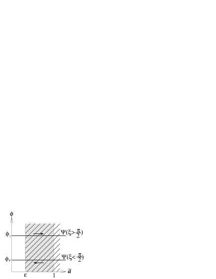
FIG. 3.: A picture of the superspace $(\tilde{a},\phi)$ near the matching region. The thick lines are the one-parameter family of configurations $(\bar{h}_{ij}(\xi),\bar{\phi}(\xi))$ in the range $\xi\in[0,\pi/2)$ and $\xi\in(\pi/2,\xi_{f}]$. The arrow indicates the direction of increase in $\xi$ along the family. The WKB approximation is valid in the hatched region and the wave function (39) is valid in the grayed region. The overlapping region is where the matching is performed.

Since Eqs. (35) and (36) have exactly the same $\tilde{a}$ dependence, the comparison of them with (39) readily gives

$$A=\epsilon E=C\,,\quad B=\epsilon(Ee^{(\nu+\frac{1}{2})\pi i}+F)=D\,,$$ (40)

independently of the choice of the operator-ordering.

Plugging this result into Eq. (28) and noting Eq. (27), we find the wave function for $\xi\in(0,\pi/2)$ as

$$\Psi(0<\xi<\pi/2)=Ne^{S_{B}/2\hbar}\exp\left[-{1\over\hbar}W_{0}^{FV}(\xi)\right]+\frac{i}{2}Ne^{-S_{B}/2\hbar}\exp\left[{1\over\hbar}W_{0}^{FV}(\xi)\right].$$ (41)

Noting the fact $W_{0}^{FV}(0)=S_{F}/2$, we connect this to the Lorentzian region $\xi<0$ of the false vacuum to obtain

$$\Psi(\xi<0) = N\exp\left[{1\over 2\hbar}(S_{B}-S_{F})\right]\left\{\exp\left[{i\over\hbar}\int^{t(\xi)}_{0}dt^{\prime}L^{FV}(t^{\prime})\right]+\exp\left[-{i\over\hbar}\int^{t(\xi)}_{0}dt^{\prime}L^{FV}(t^{\prime})\right]\right\}$$ (43)

$$+\frac{i}{2}N\exp\left[-{1\over 2\hbar}(S_{B}-S_{F})\right]\left\{\exp\left[{i\over\hbar}\int^{t(\xi)}_{0}dt^{\prime}L^{FV}(t^{\prime})\right]+\exp\left[-{i\over\hbar}\int^{t(\xi)}_{0}dt^{\prime}L^{FV}(t^{\prime})\right]\right\}\,.$$

Since $S_{B}>S_{F}$, the first two terms in the curly brackets dominate. Thus, the tunneling amplitude $\Gamma$ of the false vacuum decay is found to be

$$\Gamma\sim\frac{|\Psi(\xi_{f})|^{2}}{|\Psi(0)|^{2}}=\exp\left[-{1\over\hbar}(S_{B}-S_{F})\right].$$ (44)

This agrees with the result in the thin-wall limit. The overall behavior of the wave function is shown schematically in Fig.4, in which the normalization constant $N$ is chosen to be $\exp[-(S_{B}-S_{F})/2\hbar]$ so that the amplitude of the wave function at the false vacuum equals unity.

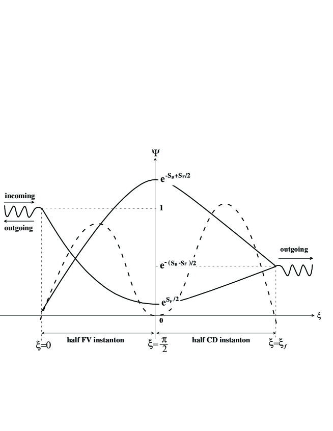
FIG. 4.: A schematic behavior of the tunneling wave function. The point $\xi=\pi/2$ is where the scale factor $a$ vanishes, and towards both right and left directions from there the 3-volume increases. The dotted curve indicates the effective potential barrier.

IV Discussion and conclusion

We have presented a new method to calculate the tunneling wave function that describes the false vacuum decay with gravity. In this method, the tunneling wave function is constructed by matching the false vacuum (FV) instanton and the Coleman-DeLuccia (CD) instanton through the point at which the scale factor vanishes. We found the resulting tunneling amplitude agrees with the naive extrapolation of the formula whose validity had been justified only in the thin-wall limit or in the flat background. Our result is a strong support for the standard interpretation that analytic continuation through the critical bubble configuration of the CD instanton describes the universe after false vacuum decay.

In our picture, the false vacuum decay with gravity becomes more or less quantum cosmological. For example, as can be seen from Fig. 4, interpreting the wave function as describing the actual tunneling path, the tunneling under consideration is quite similar to a case of standard quantum tunneling with a resonant state inside the barrier, except for the sign of the Euclidean actions $S_{F}$ and $S_{B}$ which are negative. The difference is that the resonant state here is not a state of something but the state of ‘nothing’. This gives us a very interesting picture that the false vacuum decay is first proceeded by pumping up the amplitude in the state of nothing and subsequently a universe with an expanding bubble is created from nothing.

A similar idea of joining the two instantons was previously proposed by Bousso and Chamblin in the context of path-integral approach[8]. But the principles behind his approach and ours seem rather different. Our method is completely within the scope of the standard WKB approximation, while they had to introduce a Planck size wormhole and reverse the sign the 4-volume after traversing the wormhole in an ad hoc way. Nevertheless, it is of interest to see if these two methods correspond to each other at certain level of approximations.

Recently, Rubakov and Sibiryakov proposed another method to deal with the false vacuum decay with gravity[9], by considering complex paths and adding a constraint to the action to realize the initial false vacuum state. It is, however, not clear how the complex path they considered joins the false vacuum and the critical bubble configuration, particularly because of the constraint that modifies the equations of motion.

We have demanded the wave function to have only the component describing an expanding universe after false vacuum decay. In this respect, our boundary condition is very similar to the tunneling boundary condition proposed by Vilenkin [6] in the context of quantum cosmology. However, in Vilenkin’s picture, only the wave function for an expanding universe appears in the Lorentzian region of the superspace. This means there is a steady flux coming out from the Euclidean boundaries of the superspace. On the other hand, our wave function is outgoing only for the universe after false vacuum decay. Indeed, along the line $\phi=\phi_{F}$ in the superspace, where the universe is in the false vacuum, our wave function has both expanding and contracting components. See Fig. 5. The latter feature is similar to the one of the Hartle-Hawking wave function [10]. These similarities of our wave function with both the Vilenkin and Hartle-Hawking wave functions can be seen also in Fig. 4: If we consider only the right-hand side ($\xi>\pi/2$) of the figure, it looks exactly like the cosmological wave function satisfying the Vilenkin boundary condition. In fact, the amplitude at $a=0$ ($\xi=\pi/2$) is dominated by the component that decreases exponentially as $a$ increases, as is the case of the Vilenkin wave function. On the other hand, if we consider only the left-hand side ($\xi<\pi/2$) of the figure, our wave function can be approximately regarded as a Hartle-Hawking wave function. The exponentially decreasing component becomes totally negligible when it appears in the Lorentzian region, hence it is an irrelevant component, while the exponentially increasing component dominates the wave function in the Lorentzian region, which consists of both outgoing and ingoing components with equal weight. This is the characteristic Hartle-Hawking feature.

FIG. 5.: Schematic picture of the causal structure of superspace and the one-parameter family of configurations used to construct the wave function. The Euclidean region is shaded. The lines indicated by FV and CD correspond to the configurations of the false vacuum and Coleman-DeLuccia solutions, respectively. The up or down arrows along the lines indicate the expanding or contracting components contained in the wave function.

We have considered only the leading order behavior of the WKB wave function. We need to analyze the next order to determine the quantum state of fluctuations after tunneling. It seems, however, that there is no reason to expect the result should differ from the ones obtained previously under the assumption of the Euclidean vacuum associated with the CD instanton. This is because all the properties of the quantum fluctuations are determined by the Euclidean structure of a single classical solution, which is the CD instanton, as far as we are interested only in the state after false vacuum decay: The quantum fluctuations around the CD instanton is completely decoupled from those around the FV instanton. Then once we focus only on the CD instanton, our wave function satisfies the outgoing boundary condition, and it is known to give the Euclidean vacuum state[11]. This reassures the validity of previous calculations of quantum fluctuations in the one-bubble open inflation scenario[12].

Acknowledgment

We would like to thank J. Garriga and T. Tanaka for useful discussions and comments at the early stages of this work. This work was supported in part by the Monbusho Grant-In-Aid for Scientific Research, No. 09640355.

A covariant formulation of multidimensional tunneling

Here we recapitulate the covariant formulation of the WKB wave function for multidimensional quantum tunneling developed in [4], slightly adapted to the Wheeler-DeWitt equation.

We consider the Hamiltonian in the form,

$$\hat{H}=-{\hbar^{2}}g^{\alpha\beta}(q)\frac{1}{f(q)}\nabla_{\alpha}f(q)\nabla_{\beta}+U(q)$$ (A1)

where $\{q^{\alpha}\}$ are the coordinates in the configuration space of the dynamical variables, or superspace, and $g_{\alpha\beta}$ is the superspace metric. Expanding the wave function as

$$\Psi=\exp\left[-\frac{1}{\hbar}(W_{0}+\hbar W_{1}+\cdots)\right],$$ (A2)

and inserting it into the Wheeler-DeWitt equation $\hat{H}\Psi=0$, we obtain the lowest-order WKB equation,

$$-\ g^{\alpha\beta}\nabla_{\alpha}W_{0}\nabla_{\beta}W_{0}+U(q)=0,$$ (A3)

and the first-order WKB equation,

$$-g^{\alpha\beta}\nabla_{\alpha}W_{0}\nabla_{\beta}W_{1}+\frac{1}{2}g^{\alpha\beta}\nabla_{\alpha}\nabla_{\alpha}W_{0}+\frac{1}{2}g^{\alpha\beta}\frac{\nabla_{\alpha}f(q)}{f(q)}\nabla_{\beta}W_{0}=0.$$ (A4)

Introducing a parameter $\tau$ such that

$$\frac{dq^{a}(\tau)}{d\tau}=g^{\alpha\beta}\nabla_{\beta}W_{0}\,,$$ (A5)

we obtain from Eq. (A3),

$$W_{0}=\int d\tau\,U(q(\tau)),$$ (A6)

and from Eq. (A4),

$$W_{1}=\frac{1}{2}\ln\left[\det\left[\frac{\partial q^{\beta}}{\partial\lambda^{\alpha}}\right]\sqrt{|g|}f(q)\right]+\mbox{const.},$$ (A7)

where $\{\lambda^{\alpha}\}=\{\tau,\lambda^{n}\}$ and $\{\lambda^{n}\}$ labels the different orbits of the congruence satisfying Eq. (A5) on the superspace.

For our mini-superspace system (4), the choice $\{q^{\alpha}\}=\{a,\phi\}$ leads to

$$g_{\alpha\beta}=\left(\begin{array}[]{cc}-a/\kappa&0\\ 0&2\pi^{2}a^{3}\end{array}\right)\,,\quad f(q)=a^{p-1}.$$ (A8)

The congruence containing both FV and CD instantons is expressed in the vicinity of $a=0$ as

$$a(\tau,\phi_{0})=\tau+O(\tau^{3}),\quad\phi(\tau,\phi_{0})=\phi_{0}+O(\tau^{2}).$$ (A9)

Hence a convenient choice of the label $\lambda$ of the orbits is the value of $\phi$ at $\tau=0$, $\phi_{0}$. Substituting Eqs. (A8) and (A9) into Eq. (A7), we find

$$W_{1}=\ln a^{\frac{p+1}{2}}+\mbox{const.}.$$ (A10)

Equations (A6) and (A7) give the WKB wave function to the first order,

$$\Psi=Na^{-{p+1\over 2}}\exp[-\int d\tau\,U(a(\tau),\phi(\tau))],$$ (A11)

with $U=-(a/\kappa)Q(a,\phi)$.

REFERENCES

- [1] S. Coleman and F. De Luccia, Phys. Rev. D21, 3305 (1980)
- [2] S. Coleman, Phys. Rev. D15, 2929 (1977)
- [3] T. Banks, C.M. Bender and T.T. Wu, Phys. Rev. D8, 3346 (1973); T. Banks and C.M. Bender, ibid. 8, 3366 (1973); J.L. Gervais and B. Sakita, ibid. 15, 3507 (1977); K.M. Bitar and S.J. Chang, ibid. 18, 435 (1978)
- [4] T. Tanaka, M.Sasaki and K.Yamamoto, Phys. Rev. D49, 1039 (1994)
- [5] L.G. Jensen and P.J. Steinhardt, Nucl. Phys. B237, 176 (1984)
- [6] A. Vilenkin, Phys. Rev. D30, 509 (1984); A. Vilenkin, Phys. Rev. D33, 3560 (1986)
- [7] W. Fischler, D.Morgan and J. Polchinski, Phys. Rev. D42 (1990)
- [8] R. Bousso and A. Chamblin, Phys. Rev. D59, 084004 (1999)
- [9] V.A. Rubakov and S.M.Sibiryakov, gr-qc/9905093
- [10] J.B. Hartle and S.W. Hawking, Phys. Rev. D28, 2960 (1983)
- [11] T. Vachaspati and A. Vilenkin, Phys. Rev. D37, 898 (1988)
- [12] J. Garriga, X. Montes, M. Sasaki and T. Tanaka, Nucl.Phys. B513, 343 (1998); ibid. B551, 317 (1999)