Post-Newtonian SPH calculations of binary neutron star coalescence. I. Method and first results.

Abstract

We present the first results from our Post-Newtonian (PN) Smoothed Particle Hydrodynamics (SPH) code, which has been used to study the coalescence of binary neutron star (NS) systems. The Lagrangian particle-based code incorporates consistently all lowest-order (1PN) relativistic effects, as well as gravitational radiation reaction, the lowest-order dissipative term in general relativity. We test our code on sequences of single NS models of varying compactness, and we discuss ways to make PN simulations more relevant to realistic NS models. We also present a PN SPH relaxation procedure for constructing equilibrium models of synchronized binaries, and we use these equilibrium models as initial conditions for our dynamical calculations of binary coalescence. Though unphysical, since tidal synchronization is not expected in NS binaries, these initial conditions allow us to compare our PN work with previous Newtonian results.

We compare calculations with and without 1PN effects, for NS with stiff equations of state, modeled as polytropes with $\Gamma=3$. We find that 1PN effects can play a major role in the coalescence, accelerating the final inspiral and causing a significant misalignment in the binary just prior to final merging. In addition, the character of the gravitational wave signal is altered dramatically, showing strong modulation of the exponentially decaying waveform near the end of the merger. We also discuss briefly the implications of our results for models of gamma-ray bursts at cosmological distances.

I Introduction and Motivation

Coalescing compact binaries with neutron star (NS) or black hole (BH) components provide the most promising sources of gravitational waves for detection by the large laser interferometers currently under construction, such as LIGO [1], VIRGO [2], GEO [3, 4], and TAMA [5]. In addition to providing a major new confirmation of Einstein’s theory of general relativity (GR), including the first direct proof of the existence of black holes [6, 7], the detection of gravitational waves from coalescing binaries at cosmological distances could provide accurate independent measurements of the Hubble constant and mean density of the Universe [8].

Expected rates of NS binary coalescence in the Universe, as well as expected event rates in laser interferometers, have now been calculated by many groups (see [9] for a recent review). Although there is some disparity between various published results, the estimated rates are generally encouraging. Finn & Chernoff [10] calculated that an advanced LIGO could observe as many as 20 NS merger events per year. This number corresponds to an assumed Galactic NS merger rate ${\cal R}\simeq 10^{-6}\,{\rm yr}^{-1}$ derived from radio pulsar surveys [11]. However, later revisions [12] increased this number to ${\cal R}\simeq 3\times 10^{-6}\,{\rm yr}^{-1}$, using the latest galactic pulsar population model of Ref. [13]. This value is consistent with the upper limit of ${\cal R}\lesssim 10^{-4}\,{\rm yr}^{-1}$ derived (most recently) by Arzoumanian et al. [14] on the basis of very general statistical considerations about radio pulsars, and by Kalogera & Lorimer [15], who studied constraints from supernova explosions in binaries.

Many calculations of gravitational wave emission from coalescing binaries have focused on the waveforms emitted during the last few thousand orbits, as the frequency sweeps upward from $\sim 10\,$Hz to $\sim 300\,$Hz. The waveforms in this frequency range, where the sensitivity of ground-based interferometers is highest, can be calculated very accurately by performing post-Newtonian (hereafter PN) expansions of the equations of motion for two point masses [16]. However, at the end of the inspiral, when the binary separation becomes comparable to the stellar radii (and the frequency is $\gtrsim 1\,$kHz), hydrodynamics becomes important and the character of the waveforms must change. Special purpose narrow-band detectors that can sweep up frequency in real time will be used to try to catch the last $\sim 10$ cycles of the gravitational waves during the final coalescence [17]. These “dual recycling” techniques are being tested right now on the German-British interferometer GEO 600 [4]. In this terminal phase of the coalescence, when the two NS merge together into a single object, the waveforms contain information not just about the effects of GR, but also about the interior structure of a NS and the nuclear equation of state (EOS) at high density. Extracting this information from observed waveforms, however, requires detailed theoretical knowledge about all relevant hydrodynamic processes. If the NS merger is followed by the formation of a BH, the corresponding gravitational radiation waveforms will also provide direct information on the dynamics of rotating core collapse and the BH “ringdown” (see, e.g., Ref. [6]).

Many theoretical models of gamma-ray bursts (GRBs) have also relied on coalescing compact binaries to provide the energy of GRBs at cosmological distances [18]. The close spatial association of some GRB afterglows with faint galaxies at high redshifts is not inconsistent with a compact binary origin, in spite of the large recoil velocities acquired by compact binaries at birth [19]. Currently the most popular models all assume that the coalescence leads to the formation of a rapidly rotating Kerr BH surrounded by a torus of debris. Energy can then be extracted either from the rotation of the BH or from the material in the torus so that, with sufficient beaming, the gamma-ray fluxes observed from even the most distant GRBs can be explained [20]. Here also, it is important to understand the hydrodynamic processes taking place during the final coalescence before making assumptions about its outcome. For example, contrary to widespread belief, it is not clear that the coalescence of two $1.4\,M_{\odot}$ NS will form an object that must collapse to a BH, and it is not certain either that a significant amount of matter will be ejected during the merger and form an outer torus around the central object (see Sec. III below and Ref. [21]).

The final hydrodynamic merger of two compact objects is driven by a combination of relativistic and fluid effects. Even in Newtonian gravity, an innermost stable circular orbit (ISCO) is imposed by global hydrodynamic instabilities, which can drive a close binary system to rapid coalescence once the tidal interaction between the two stars becomes sufficiently strong. The existence of these global instabilities for close binary equilibrium configurations containing a compressible fluid, and their particular importance for binary NS systems, was demonstrated for the first time by Rasio & Shapiro (Ref. [22], hereafter RS1–3 or collectively RS) using numerical hydrodynamic calculations. These instabilities can also be studied using analytic methods. The classical analytic work for close binaries containing an incompressible fluid (e.g., Ref. [23]) was extended to compressible fluids in the work of Lai, Rasio, & Shapiro (Ref. [24], hereafter LRS1–5 or collectively LRS). This analytic study confirmed the existence of dynamical instabilities for sufficiently close binaries. Although these simplified analytic studies can give much physical insight into difficult questions of global fluid instabilities, 3D numerical calculations remain essential for establishing the stability limits of close binaries accurately and for following the nonlinear evolution of unstable systems all the way to complete coalescence.

A number of different groups have now performed such calculations, using a variety of numerical methods and focusing on different aspects of the problem. Nakamura and collaborators (see [25] and references therein) were the first to perform 3D hydrodynamic calculations of binary NS coalescence, using a traditional Eulerian finite-difference code. Instead, RS used the Lagrangian method SPH (Smoothed Particle Hydrodynamics). They focused on determining the ISCO for initial binary models in strict hydrostatic equilibrium and calculating the emission of gravitational waves from the coalescence of unstable binaries. Many of the results of RS were later independently confirmed by New & Tohline [26] and Swesty et al. [27], who used completely different numerical methods but also focused on stability questions, and by Zhuge, Centrella, & McMillan [28, 29], who also used SPH. Davies et al. [30] and Ruffert et al. [31, 32] have incorporated a treatment of the nuclear physics in their hydrodynamic calculations (done using SPH and PPM codes, respectively), motivated by cosmological models of GRBs. All these calculations were performed in Newtonian gravity, with some of the more recent studies adding an approximate treatment of energy and angular momentum dissipation through the gravitational radiation reaction [33].

Zhuge et al. [28, 29] and Ruffert et al. [31, 32] also explored in detail the dependence of the gravitational wave signals on the initial NS spins. Because the viscous timescales for material in the NS is much longer than the dynamical timescale during inspiral, it is generally assumed that NS binaries will be non-synchronized during mergers. It is generally found than non-synchronized binaries yield less mass loss from the system, but very similar gravity wave signals, especially during the merger itself when the gravity wave luminosity is highest [31].

All recent hydrodynamic calculations agree on the basic qualitative picture that emerges for the final coalescence. As the ISCO is approached, the secular orbital decay driven by gravitational wave emission is dramatically accelerated (see also LRS2, LRS3). The two stars then plunge rapidly toward each other, and merge together into a single object in just a few rotation periods. In the corotating frame of the binary, the relative radial velocity of the two stars always remains very subsonic, so that the evolution is nearly adiabatic. This is in sharp contrast to the case of a head-on collision between two stars on a free-fall, radial orbit, where shock heating is very important for the dynamics (see, e.g., RS1 and Ref. [34]). Here the stars are constantly being held back by a (slowly receding) centrifugal barrier, and the merging, although dynamical, is much more gentle. After typically $1-2$ orbital periods following first contact, the innermost cores of the two stars have merged and the system resembles a single, very elongated ellipsoid. At this point a secondary instability occurs: mass shedding sets in rather abruptly. Material (typically $\sim 10$% of the total mass) is ejected through the outer Lagrange points of the effective potential and spirals out rapidly. In the final stage, the inner spiral arms widen and merge together, forming a nearly axisymmetric torus around the inner, maximally rotating dense core.

In GR, strong-field gravity between the masses in a binary system is alone sufficient to drive a close circular orbit unstable. In close NS binaries, GR effects combine nonlinearly with Newtonian tidal effects so that the ISCO should be encountered at larger binary separation and lower orbital frequency than predicted by Newtonian hydrodynamics alone, or GR alone for two point masses. The combined effects of relativity and hydrodynamics on the stability of close compact binaries have only very recently begun to be studied, using both analytic approximations (basically, PN generalizations of LRS; see, e.g., [35, 36], as well as numerical calculations in 3D incorporating simplified treatments of relativistic effects (e.g., [37, 38]). Several groups have been working on a fully relativistic calculation of the final coalescence, combining the techniques of numerical relativity and numerical hydrodynamics in 3D [39, 40]. However this work is still in its infancy, and only preliminary results of test calculations have been reported so far. It should be noted that 1PN calculations performed by Taniguchi and collaborators [41] to study the location of the ISCO for corotating and irrotational binaries find that the ISCO moves inwards as post-Newtonian corrections are increased, due primarily to the effect of 1PN potentials with momentum-based source terms present in the system. Similarly, Buonanno and Damour [42] find that the ISCO for point masses in a binary under GR moves inwards with increasingly massive objects.

The middle ground between Newtonian and fully relativistic calculations is the study of the hydrodynamics in PN gravity. Formalisms exist describing not only all lowest-order corrections (1PN) to Newtonian gravity, but also the lowest-order (2.5PN) effects of the gravitational radiation reaction [43, 44]. Such calculations have been undertaken by Shibata, Oohara & Nakamura [45] using an Eulerian grid-based code, and more recently by Ayal et al. [46] using SPH. This paper is the first of a series in which we will present a comprehensive study of the hydrodynamics of compact binary coalescence using a new PN version of a parallel SPH code which we have been developing over the past two years. This work will be the natural extension to PN gravity of the original Newtonian study by RS.

PN calculations of NS binary coalescence are particularly relevant for stiff NS EOS. Indeed, for most recent stiff EOS, the compactness parameter for a typical $1.4\,M_{\odot}$ NS is in the range $GM/Rc^{2}\simeq 0.1-0.2$, justifying a PN treatment. After complete merger, an object close to the maximum stable mass is formed, with $GM/Rc^{2}\simeq 0.3-0.5$, and relativistic effects become much more important. However, even then, a PN treatment can remain qualitatively accurate if the final merged configuration is stable to gravitational collapse on a dynamical timescale (see the discussion in Sec. III D). Most recent theoretical calculations (e.g., the latest version of the Argonne/Urbana EOS; see Ref. [47]) and a number of recent observations (e.g., of cooling NS; see Ref. [48]) provide strong support for a stiff NS EOS. In this paper we represent NS with stiff EOS by simple polytropes with an adiabatic exponent $\Gamma=3$ (i.e., the EOS is of the form $p_{*}=kr_{*}^{\Gamma}$, where $p_{*}$ is the pressure, $r_{*}$ is the rest-mass density, and $k$ is a constant; see RS2 and LRS3, who obtain $\Gamma\simeq 3$ for the best polytropic fit to recent stiff NS EOS).

The most significant problem facing PN hydrodynamic simulations is the requirement that all 1PN quantities be small compared to unity. Unfortunately, this precludes the use of realistic NS models. Shibata, Oohara & Nakamura [45] computed 1PN mergers of polytropes with $\Gamma=5/3$ and a compactness $GM/Rc^{2}=0.03$, leaving out the effects of the gravitational radiation reaction. Ayal et al. [46] performed calculations for polytropes with $\Gamma=1.6$ or $\Gamma=2.6$ and compactness values in the range $GM/Rc^{2}\simeq 0.02-0.04$, including the effects of the gravitational radiation reaction. For comparison, a realistic NS of mass $M=1.4\,M_{\odot}$ and radius $R=10\,{\rm km}$ has $GM/Rc^{2}=0.2$, i.e., about an order of magnitude larger. Unfortunately, performing calculations with artificially small values of $GM/Rc^{2}$ also has the side effect of dramatically inhibiting the radiation reaction, which scales as $(GM/Rc^{2})^{2.5}$.

Our PN SPH code combines a new parallel version of the Newtonian SPH code used by RS with a treatment of PN gravity based on the formalism of Blanchet, Damour, and Schäfer (Ref. [44], hereafter BDS). Our calculations include all 1PN effects, as well as a PN treatment of the gravitational radiation reaction. We have also developed a relaxation technique by which accurate quasi-equilibrium configurations can be calculated for close binaries in PN gravity. These serve as initial conditions for our hydrodynamic coalescence calculations. In addition, we present in this paper a simple solution to the problem of suppressed radiation reaction for models of NS with unrealistically low values of $GM/Rc^{2}$.

The outline of our paper is as follows. Section II presents our numerical methods, including the description of our new PN SPH code, a discussion of the advantages of using SPH for this work, and the steps taken to make our results as realistic as possible. More details on the methods and our treatment of the initial conditions are given in the appendices. Section III presents our initial results, based on two large-scale simulations, with and without 1PN effects. These are performed for synchronized initial binaries containing two identical polytropes with $\Gamma=3$. In future papers, we will study systematically the dependence of these results on the NS EOS (by varying $GM/Rc^{2}$ and $\Gamma$, and using more realistic, tabulated EOS for nuclear matter at high density), the NS spins (allowing for nonsynchronized initial conditions), and the binary mass ratio. Motivation for this future work as well as a brief summary of our present results are presented in Section IV.

II Numerical Method

A The SPH Code

Smoothed Particle Hydrodynamics (SPH) is a Lagrangian method ideally suited to calculations involving self-gravitating fluids moving freely in 3D. The key idea of SPH is to calculate pressure gradient forces by kernel estimation, directly from the particle positions, rather than by finite differencing on a grid (see, e.g., [49], for recent reviews on the method). SPH was introduced more than 20 years ago by Lucy, Monaghan, and collaborators [50], who used it to study dynamical fission instabilities in rapidly rotating stars. Since then, a wide variety of astrophysical fluid dynamics problems have been tackled using SPH (see Ref. [51] for an overview).

Because of its Lagrangian nature, SPH presents some clear advantages over more traditional grid-based methods for calculations of stellar interactions. Most importantly, fluid advection, even for stars with a sharply defined surface such as NS, is accomplished without difficulty in SPH, since the particles simply follow their trajectories in the flow. In contrast, to track accurately the orbital motion of two stars across a large 3D grid can be quite tricky, and the stellar surfaces then require a special treatment (to avoid “bleeding”). SPH is also very computationally efficient, since it concentrates the numerical elements (particles) where the fluid is at all times, not wasting any resources on emty regions of space. For this reason, with given computational resources, SPH provides higher averaged spatial resolution than grid-based calculations, although Godunov-type schemes such as PPM typically provide better resolution of shock fronts (this is certainly not a decisive advantage for binary coalescence calculations, where no strong shocks ever develop). SPH also makes it easy to track the hydrodynamic ejection of matter to large distances from the central dense regions. Sophisticated nested-grid algorithms are necessary to accomplish the same with grid-based methods.

Our simulations were performed using a modified version of an SPH code that was originally designed to perform 3D Newtonian calculations of stellar interactions (see Ref. [52] and RS1). Although the fluid description is completely Lagrangian, the gravitational field in our code (including PN terms) is calculated on a 3D grid using an FFT-based Poisson solver. Our Poisson solver is based on the FFTW of Frigo & Johnson [53], which features fully parallelized real-to-complex transforms. Boundary conditions are handled by zero-padding all grids, which has been found to produce accurate results and to be the most computationally efficient method (see also [27]). Since we are primarily interested in the gravitational wave emission, which originates mainly from the inner dense regions of NS mergers, we fix our grid boundaries to be $\pm 4$ NS radii in all directions from the center of mass. Particles that fall outside these boundaries are treated by including a simple monopole gravitational interaction with the matter on the grid. Our code has been developed on the SGI/Cray Origin 2000 parallel supercomputer at NCSA. MPI (the Message Passing Interface) reduces the memory overhead of the code by splitting all large grids among the processors. All hydrodynamic loops over SPH particles and their neighbors have also been fully parallelized using MPI, making our entire code easily portable to other parallel supercomputers. The parallelization provides nearly linear speedup with increasing number of processors up to $\sim 10$, with a progressive degradation for larger numbers.

For more details on the Newtonian version of the code, and extensive results from test calculations, see Ref. [54].

B The Blanchet, Damour, and Schäfer PN Formalism with SPH

To investigate the hydrodynamics of NS binary coalescence beyond the Newtonian regime, the equations of RS were modified to account for PN effects described by the formalism of BDS, converted into a Lagrangian, rather than Eulerian form. The main equations and definitions of quantities appearing in the BDS formalism are summarized briefly in Appendix A. The formalism is correct to first (1PN) order, with all new forces calculated from eight additional Poissson-type equations with compact support, allowing for the computation of all 1PN terms using the same FFT-based convolution algorithm as for the Newtonian Poisson solver. PN corrections to hydrodynamic quantities are calculated by the SPH method, i.e., by summations over particles. Dissipation of energy and angular momentum by gravitational radiation reaction is included to lowest (2.5PN) order, requiring the solution of one additional Poisson-type equation.

The key changes to the BDS formalism involve a conversion to quantities based on SPH particle positions, rather than grid points. In the discussion that follows, $a$ and $b$ refer to quantities defined for particles, or particle neighbors, while $i$ and $j$ are spatial indices. The rest-mass density is calculated at each particle position as a weighted sum over the masses of neighboring particles,

$$r_{*}^{(a)}=\sum_{b}m_{b}W_{ab},$$ (1)

where $m_{a}$ is the rest mass of particle $a$, and the weights are given in terms of a smoothing kernel $W(\vec{r},h)$ by

$$W_{ab}=\frac{1}{2}[W(|\vec{r}_{(a)}-\vec{r}_{(b)}|,h_{a})+W(|\vec{r}_{(a)}-\vec{r}_{(b)}|,h_{a})].$$ (2)

Here $h_{a}$ is the smoothing length for particle $a$, which is updated after every iteration so as to keep the number of neighbors as close as possible to a designated optimal value $N_{N}$. The form of the SPH kernel $W$ used in our calculations is the same standard third-order spline used by RS (and most other current implementations of SPH). This kernel is spherical and goes to zero for $r>2h$.

The total mass-energy of the system can be calculated as

$$M_{g}=\int d^{3}x~{}r_{*}(1+\delta)=\sum_{b}m_{b}(1+\delta_{b}),$$ (3)

where $\delta$ is a 1PN correction defined in Eq. (A12), while the total rest mass is

$$M=\int d^{3}x~{}r_{*}=\sum_{b}m_{b}.$$ (4)

In our simple polytropic models of NS, the pressure is calculated from the local density as

$$p_{*}^{(a)}=k_{a}(r_{*}^{(a)})^{\Gamma}$$ (5)

where $k_{a}$ is a function of the specific entropy of the particle, and $\Gamma$ is the adiabatic exponent. The standard Newtonian pressure force is given by

$$F_{i}^{hydro}=-\frac{\partial_{i}p_{*}^{(a)}}{r_{*}^{(a)}}=-\sum_{b}m_{b}\left(\frac{p_{*}^{(a)}}{(r_{*}^{(a)})^{2}}+\frac{p_{*}^{(b)}}{(r_{*}^{(b)})^{2}}\right)\nabla_{i}W_{ab}.$$ (6)

In the absence of artificial viscosity (AV), entropy is conserved and $k_{a}$ is constant throughout the simulation. If AV is included, the first law of thermodynamics can be expressed as

$$\frac{dk_{a}}{dt}=\frac{\Gamma-1}{2(r_{*}^{(a)})^{\Gamma-1}}\sum_{b}m_{b}\Pi_{(a,b)}(\vec{w}_{(a)}-\vec{w}_{(b)})\cdot\nabla_{i}W_{ab},$$ (7)

with a corresponding force on particles given by

$$F_{i}^{AV}=-\sum_{b}m_{b}\Pi_{(a,b)}\nabla_{i}W_{ab}.$$ (8)

The expression for $\Pi_{(a,b)}$ depends on the particular choice of AV. We use the form proposed by Balsara [55], which gives

$$\Pi_{(a,b)}=\left(\frac{p_{*}^{(a)}}{(r_{*}^{(a)})^{2}}+\frac{p_{*}^{(b)}}{(r_{*}^{(b)})^{2}}\right)(-\alpha^{\prime}\mu_{(a,b)}+\beta^{\prime}\mu_{(a,b)}^{2}),$$ (9)

where $\mu_{(a,b)}$ is a measure of the rate of convergence in the flow. The exact definition of $\mu_{(a,b)}$ can be found in Eqs. (15–19) of Lombardi et al. [54], who also show that the optimal choice of the numerical coefficients is $\alpha^{\prime}=\beta^{\prime}=\Gamma/2$. This form was shown to handle shocks properly and minimize the amount of spurious mixing and numerical shear viscosity.

For the PN pressure force (Eq. A17), we now find

$$F_{i}^{press}=-(1+\frac{\alpha}{c^{2}})(F_{i}^{hydro}+F_{i}^{AV})-\frac{1}{c^{2}}\frac{p_{*}}{r_{*}}\partial_{i}\alpha,$$ (10)

where $\alpha/c^{2}\ll 1$ is a PN correction. In the calculation of $\partial_{i}\alpha=(2-3\Gamma)\partial_{i}U_{*}-\frac{\Gamma}{2}\partial_{i}w^{2}$, we must take a derivative of the local dynamic velocity-squared field, which we do by SPH summations, i.e., we first write

$$\partial_{i}(w^{2})=\frac{1}{r_{*}}(\partial_{i}(r_{*}w^{2})-w^{2}\partial_{i}r_{*}),$$ (11)

and we then calculate the derivative terms as

$$\partial_{i}r_{*}^{(a)} = \sum_{b}m_{b}\partial_{i}W_{ab},$$ (12)

$$\partial_{i}(r_{*}w^{2})^{(a)} = \sum_{b}m_{b}w_{(b)}^{2}\partial_{i}W_{ab}.$$ (13)

The nine Poisson-type equations in the full PN formalism of BDS are all solved by the same FFT convolution method. All 3D grids used by the Poisson solver are distributed among the processors in the z-direction. Real-to-complex transforms are computed using the rfftwnd_mpi package of the FFTW library [53]. The source terms of the Poisson equations that do not contain density derivatives, Eqs. (A5,A6,A8), are laid down on the grid by a cloud-in-cell method. All integrals over the density distribution are converted into sums over particles, e.g.,

$$U_{*}(x)=\int d^{3}x\frac{r_{*}(x^{\prime})}{|x-x^{\prime}|}\rightarrow\sum_{b}\frac{m_{b}}{|x-x_{b}|}.$$ (14)

Source terms containing density derivatives are calculated by finite differencing on the grid, rather than by SPH-based derivatives at particle positions. This has two benefits. First, for integrals of the type

$$\Phi=\int d^{3}x~{}\partial_{i}r_{*}\ldots$$ (15)

we cannot convert directly from a volume integral to a sum over discrete particle masses. Second, it guarantees that the volume integral of the source term vanishes in Eqs. (A7,A16), as it should. Derivatives of the potentials are computed by finite differencing on the grid, and then interpolated between grid points to assign values at SPH particle positions.

The calculation of the quadrupole tensor and its derivatives are unchanged in a Lagrangian formulation. When calculating the third derivative, however, we found it advantageous to take the SPH expression for the second derivative of the quadrupole tensor (RS1),

$$\ddot{Q}_{ij}=\sum_{b}m_{b}(v^{(b)}_{i}v^{(b)}_{j}+x_{i}^{(b)}\partial_{j}U_{*}+x_{j}^{(b)}\partial_{i}U_{*}),$$ (16)

and numerically differentiate once with respect to time. The resulting expression differs from the third derivative expression given in BDS by a term of $O\left(v^{2}/c^{2}\right)$, but all radiation reaction terms into which it enters already contain factors of $O\left(v^{5}/c^{5}\right)$. While only approximate, this method proved more stable since it does not require the numerical evaluation of several second derivatives on a grid.

For calculations in which we include the radiation reaction, but ignore 1PN corrections, all terms containing a factor of $1/c^{2}$ in Appendix A can be ignored. In this case our equations reduce to those of the purely Newtonian case, with two exceptions. First, we include $F_{i}^{reac}$ (Eq. A19) in the SPH equations of motion, replacing Eq. (A21) by

$$\dot{w_{i}}=-\frac{\partial_{i}p_{*}}{r_{*}}+\partial_{i}U_{*}+F^{reac}_{i}.$$ (17)

Second, the relationship between the particle velocity $\vec{v}$ and momentum $\vec{w}$ is given by

$$v_{i}=w_{i}+\frac{4}{5}\frac{G}{c^{5}}Q^{[3]}_{ij}w_{j}.$$ (18)

This has beeen shown [31] to give the correct energy loss rate as predicted by the classical quadrupole formula,

$$\frac{dE}{dt}=\frac{1}{5}\frac{G}{c^{5}}<Q^{[3]}_{ij}Q^{[3]}_{ij}>.$$ (19)

Ignoring 1PN terms reduces the number of Poisson equations to be solved per iteration from nine to two. The obvious advantage is a proper handling of the dissipative PN effects, while leaving the hydrodynamic equations in a simple form that can be directly compared to the Newtonian case. In addition, because the corrections are $O(v^{5}/c^{5})$, the radiation reaction terms always remain small, even when 1PN corrections would be large.

We have performed a number of test calculations to establish the accuracy of our treatment of PN effects in the SPH code. These include tests for single rotating and nonrotating polytropes in PN gravity, which we have compared to well-known analytic and semi-analytic results [56]. In particular, we have verified that our code reproduces correctly the dynamical stability limit to radial collapse for a single PN polytrope with $\Gamma=5/3$ (see Sec. B 1).

C A Hybrid 1PN/2.5PN Post-Newtonian Formalism

Throughout this paper, unless otherwise specified, we use units in which Newton’s gravitational constant $G$, and the rest mass $M$ and radius $R$ of a single, spherical NS are set equal to unity. In Newtonian physics, this leads to a scale-free calculation (RS). When we include PN effects, specifying the physical mass and radius of the NS then sets the value of the speed of light $c$, and the magnitude of all PN terms. In our units, the compactness ratio $GM/Rc^{2}$ of a NS is expressed simply as $1/c^{2}$.

The equations of BDS assume that all 1PN corrections are small. As mentioned in Sec. 1, this places a rather severe constraint on the allowed NS mass and radius, since

$$\frac{1}{c^{2}}=0.14\left(\frac{M}{1.5\,M_{\odot}}\right)\left(\frac{15\,{\rm km}}{R}\right).$$ (20)

If, for example, we estimate the potential at the center of the star as $U_{*}/c^{2}\simeq 1.5/c^{2}=0.21$ (Eq. A5), which is appropriate for $\Gamma=3$ models, we find that our “first-order” correction term $\alpha/c^{2}$ (Eq. A10), with $\Gamma=3$ and no internal motions, is

$$\frac{\alpha}{c^{2}}=(2-3\Gamma)\frac{U_{*}}{c^{2}}=-7\frac{U_{*}}{c^{2}}\simeq-1.5.$$ (21)

This is clearly problematic since the derivation of the BDS formalism assumes that $|\alpha|/c^{2}\ll 1$. For a fixed radius of $15\,$km and $\Gamma=3$, a NS mass $<0.9\,M_{\odot}$, or $1/c^{2}<0.09$ is required to keep $|\alpha|<1$. This problem is less severe for a lower value of $\Gamma$, since the coefficient of $\alpha$ is then smaller. For $\Gamma=5/3$, we have $\alpha=-3U_{*}$, but these configurations are known to be unstable against gravitational collapse for compactness parameters $1/c^{2}\gtrsim 0.14$ (See, e.g., Ref. [56], and Sec. B 1). These problems are the reason why previous PN hydrodynamic simulations of NS binary coalescence have used unrealistic NS models with low masses and large radii. In practice, we find that we cannot calculate reliably NS mergers including 1PN corrections, unless $1/c^{2}\lesssim 0.05$, or $c\gtrsim 4$. With such a small compactness parameter, radiation reaction effects would then be suppressed by a factor $\sim 2^{5}=32$.

Recognizing that the 1PN and 2.5PN terms describe essentially independent phenomena, and that the proper form for energy and angular momentum loss holds even if 1PN corrections are ignored, we adopt a hybrid scheme. Specifically, in this paper, we set $c=4.47\equiv c_{1PN}$ for all 1PN corrections, which is unphysically large, but we use a physically realistic value of $c=2.5\equiv c_{2.5PN}$ for the 2.5PN corrections, corresponding, for example, to a NS mass $M=1.5\,M_{\odot}$ with radius $R=13.9\,{\rm km}$. We feel that this hybrid formulation provides a reasonable trade-off between physical reality and the limitations of the 1PN approximation.

Note that this method should better extrapolate toward physical reality, compared with unrealistically undercompact NS models. If $0+2.5$PN simulations are interpreted as taking the limit $c_{1PN}\rightarrow\infty$ for the 1PN corrections, we see that by reducing the compactness in both the $0+2.5$PN and $0+1+2.5$PN cases, the value of $c_{2.5PN}$ is fixed at an unphysical value while $c_{1PN}$ is varied, which can never truly extrapolate to the physical case. By setting $c_{2.5PN}$ to a realistic physical value while varying $c_{1PN}$, we may be able to extrapolate our results toward a correct physical limit. However, a disadvantage of this approach is that it does not allow for direct quantitative comparison with full GR simulations of binary NS coalescence. In these simulations, which essentially handle corrections to all orders simultaneously, separation into various PN orders has no meaning.

D Initial Conditions

In addition to its normal use for dynamical calculations, our SPH code can also be used to construct hydrostatic equilibrium configurations in 3D, which provide accurate initial conditions for binary coalescence calculations. This is done by adding artificial friction terms to the fluid equations of motion and forcing the system to relax to a minimum-energy state under appropriate constraints (RS). The great advantage of using SPH itself for setting up equilibrium solutions is that the dynamical stability of these solutions can then be tested immediately by using them as initial conditions for dynamical SPH calculations. Very accurate 3D equilibrium solutions can be constructed using such relaxation techniques, with the virial theorem satisfied to better than 1 part in $10^{3}$ and excellent agreement found with known quasi-analytic solutions in both Newtonian (LRS1, LRS4, RS2) and PN gravity [36]. The careful construction of accurate quasi-equilibrium initial conditions is a distinguishing feature of both our previous Newtonian calculations (RS) and our new PN calculations of binary coalescence. In contrast, most other studies have used very crude initial conditions, placing two spherical stars in a close binary orbit, and, for calculations that went beyond Newtonian gravity, adding the inward radial velocity for the inspiral of two point masses. As demonstrated in Sec. III A, this leads to a significantly slower inspiral rate. Moreover, spurious fluid motions are created as the stars respond dynamically to the sudden appearance of the strong tidal force. These can in turn corrupt the gravitational radiation waveforms. Spurious velocities have additional effects in the full 1PN case, where spurious motions enter repeatedly into the evolution equations, by propagating through the 1PN quantities $\alpha$, $\beta$, and $\delta$ (Eqs. A10,A11,A12). A specific cause of worry is the influence of velocities adding to $\delta$, which affects not only the self-gravity of the stars, but also their mutual gravitational attraction.

We have developed a method, described in detail in Appendix B, that allows for more realistic initial conditions for PN synchronized binaries. It reduces dramatically the initial oscillations around equilibrium when the dynamical calculation is started. Since the method varies rather significantly between the full $1PN+2.5PN$ formalism and the Newtonian with radiation reaction formalism, we handle the two cases separately. For the Newtonian case, radiation reaction plays no role in the relaxation, entering only into the initial values of the velocity and momentum, $\vec{v}$ and $\vec{w}$ (Eq. A22), upon the start of the dynamical run. The 1PN case is considerably more complicated, requiring the construction of static single star models, which are then input into a PN binary relaxation scheme.

III Results

We have performed two large-scale hydrodynamic simulations of NS binary coalescence, with and without the 1PN correction terms of BDS. Both simulations included radiation reaction throughout the entire run, treated in the formalism of Appendix A. Hereafter, we refer to these two runs as the Newtonian (N) and post-Newtonian (PN) runs, noting that the N simulation did include 2.5PN effects.

For both runs, we used 50,000 particles per NS (total of $10^{5}$), with a $\Gamma=3$ polytropic EOS. The two NS are identical. Synchronized rotation was assumed in the initial condition. The optimal number of neighbors for each SPH particle was set to 100. Shock heating, which plays a completely negligible role in the case studied here, was ignored and therefore the SPH AV was turned off. All Poisson equations were solved on grids of size $256^{3}$, including the added space necessary for zero-padding. For the 1PN run, we used a compactness parameter $1/c_{1PN}^{2}=0.05$ (see Sec. IIC). In both runs, we used $c_{2.5PN}=2.5$ in calculating radiation reaction terms. The N run required a total of 600 CPU hours and the PN run 1200 hours on the NCSA Origin2000, including the relaxation phase. Particle plots illustrating qualitatively the evolution of the system are shown in Fig. 1 (N run) and Fig. 2 (PN run).

A Dynamical Instability and the Inspiral Process

It was shown by RS and LRS that equilibrium configurations for close binary NS become dynamically unstable when the separation $r$ is less than a critical value. For Newtonian, synchronized, equal-mass binaries with $\Gamma=3$, the ISCO is at $r=2.95\,R$. Purely Newtonian calculations for binaries starting from equilibrium configurations with a separation larger than this value will show no evolution in the system. Binaries starting from a smaller separation, though, are dynamically unstable, and coalesce within a few orbital periods, even without the energy and angular momentum loss due to radiation reaction (RS,[26, 27]).

In simulations with radiation reaction included, coalescence will always be the end result. The limiting factor on how large to make the initial separation is the computing time required for the binary orbit to slowly spiral inward. Ideally, one should make sure that the stars are in quasi-equilibrium when the orbit approaches the ISCO and the inspiral timescale undergoes a shift from the slow radiation-reaction timescale to the much faster dynamical timescale.

Since the effective gravitational attraction between two stars is increased by PN effects, we expect the ISCO to move outwards when 1PN corrections are included. This was demonstrated by Lombardi, Rasio, & Shapiro [54], who used the same energy variational method as LRS to find equilibrium configurations for binary NS models including 1PN corrections. Taking into account these results, we used an initial separation of $r_{0}=3.1\,R$ for our N simulation, and $r=4.0\,R$ for the PN simulation. As a consequence, there is an ambiguity in the relative time between the two runs, which we resolve by adjusting the initial time of the N run such that the maximum gravity wave luminosity occurs at the same time in both the N and PN runs. This was found to require shifting the time in the N run backwards so that it starts at $t=-13$, while the PN run starts at $t=0$.

In Fig. 3, we show the evolution of the center-of-mass binary separation during the initial inspiral phase for our N and PN runs. Fig. 4 shows the inspiral phase of the N run, as well as the inspiral tracks predicted by the classical quadrupole formula for two point masses, and by the methods of LRS3 for two corotating spheres and two ellipsoids. We note that the results of LRS3 predict for extended objects a significantly more rapid inspiral rate, which is confirmed by the numerical run. In addition, we note that the approach of the ISCO is clearly visible in the plots, where the inspiral rate switches from the slow radiation-reaction-driven orbital decay to the faster dynamical infall. This appears to happen at $r\simeq 2.7\,R$ in the N case, in good agreement with previous results.

Comparing the PN run to the N run, we see that the stability limit must lie at a considerably larger separation. This agrees with the results of Lombardi et al. [54], who find that PN corrections not only move the ISCO outward, but also flatten out the equilibrium binary energy curve $E(r)$ near the stability limit (where $E(r)$ reaches a minimum). Following the arguments of LRS3, we conclude that unstable inspiral begins when the differential change in binary energy as a function of separation becomes smaller than the energy loss rate to gravitational radiation. The condition for unstable inspiral, expressed as

$$\frac{dE}{dr}\ll\frac{dE_{GW}}{dt}\left(\frac{dr}{dt}\right)^{-1},$$ (22)

is then encountered further outside the ISCO (as determined for binaries in strict equilibrium), since PN corrections decrease the left-hand side. This effect can also be seen in the results of Ayal et al. [46] by careful examination of their Fig. 5a. Even though the binary separation in their PN run has a large initial oscillation, caused by the use of non-equilibrium initial conditions, it still converges at a much more rapid rate than in their corresponding Newtonian model.

Even though the effective stability limits of N and PN binaries differ by a large amount, their actual inspiral velocities are essentially the same from the moment of first contact, at a separation of $r\simeq 2.5\,R$, until the merger of the NS cores. The only significant difference is the break in the inspiral velocity for the N run at $t\simeq 20$, which occurs as the cores start to come into direct contact with each other. The lack of this feature in the PN run will be explained in Sec. III B.

B Coalescence

In Fig. 5, we show the time evolution of the maximum density in both runs. The maximum density is at the center of either star initially, but it shifts eventually to the center of the merger remnant. The initial oscillations with a period of $T\simeq 2-3$ correspond to the fundamental radial pulsations of the polytropes, and represent the errors resulting from small departures from strict equilibrium in the initial conditions. We see that $\delta\rho/\rho\simeq 0.01$ and $0.05$, respectively, for the N and PN runs, which provides a measure of the numerical accuracy of the initial conditions.

As the binary system contracts to separations of $r\lesssim 2.7\,R$, we see a rather sudden and rapid decrease in the maximum density found at the core of each star, corresponding closely with the moment of first contact of the two stars, after which the cores get tidally stretched. For the PN run, this follows a gradual increase in the average density maximum, which is caused by the contraction of each NS in response to the growing gravitational potential of its companion, rather than a pure tidal effect. This effect, which seems to result primarily from the weakening of the pressure force in Eq. (A17) as $\alpha$ becomes more negative in response to the growing gravitational potential (Eq. A10), was also seen by Ayal et al. in one of their runs (Ref. [46], see their Fig. 6, run P3). When the center of mass separation reaches a value of $r\simeq 2.0\,R$ the maximum density stops decreasing, turning around and increasing sharply as the cores come into direct contact and merge.

In Fig. 6, we show the gravity wave signatures of both runs. The waveforms in the two polarizations of gravitational radiation are calculated for an observer at a distance $d$ along the rotation axis of the system in the quadrupole approximation,

$$c^{4}(d\,h_{+}) = \ddot{Q}_{xx}-\ddot{Q}_{yy}$$ (23)

$$c^{4}(d\,h_{\times}) = 2\ddot{Q}_{xy}.$$ (24)

In Fig. 7 we show the corresponding gravity wave luminosity of the system, given by

$$c^{5}L_{GW}=\frac{1}{5}\left\langle Q^{[3]}_{ij}Q^{[3]}_{ij}\right\rangle.$$ (25)

We see that, as the inner NS cores merge, the gravity wave luminosity peaks for both runs, with the characteristic frequency of the waves increasing like (twice) the rotation frequency of the system. This frequency increase is more rapid in the PN case, since the inspiral is faster.

After $t\simeq 30$, the evolution of the N binary is rather straightforward. A triaxial object is formed at the center of the system, with spiral outflows emanating from the outer parts of each star. The spiral arms remain coherent for several windings before slowly dissipating, and finally leaving a low-density halo of material in the region $r/R\simeq 2-15$. During this time, the central triaxial object acts as the predominant source for the gravity waves as it spins down, leading to a characteristic damped oscillatory signature, at a luminosity approximately $1/30$ that of the peak. The rise in central density from the initial value at $t=0$ to the final value at $t=80$ is consistent with what is expected from the mass-radius relation for a Newtonian polytrope with $\Gamma=3$.

This simple picture, which is familiar from many previous Newtonian simulations, is seen to break down when 1PN effects are taken into account. As is clear from Fig. 2 ($t=12$), just prior to the final coalescence, 1PN effects cause the long axis of each star to rotate forward relative to the binary axis, so that the inner part of each star leads the center of mass in the orbital rotation. This dynamical tidal lag is expected from the rapidly changing tidal forces during the final inspiral phase (LRS5). It is not to be confused with the tidal lag produced by viscous dissipation in nonsynchronized binaries (see, e.g., Ref. [57]). The dynamical tidal lag angle can be estimated analytically for a Newtonian binary whose orbit decays slowly by gravitational wave emission. Using Eq. (9.21) of LRS5, we estimate a lag angle $\alpha_{t}\simeq 0.01$ for $1/c^{2}=0.16$ and $r\simeq 2R$. This is in agreement with the very small lag angle observed in our N run (barely visible at $t=12$ in Fig.  1). In contrast, from our PN run, we find $\alpha_{t}\simeq 0.14$, indicating that the more rapid inspiral can dramatically increase this effect.

As the PN merger proceeds, material from the leading edge of each star wraps around the other, so that the cores simply slide past each other instead of striking more nearly head-on as in the N case. As this happens around $t\simeq 25$, the maximum density drops slightly, and the gravity wave luminosity rises again, reaching a second peak at $t\simeq 35$, with a maximum luminosity $L_{2}=0.65\,L_{1}$ compared to the first peak of luminosity $L_{1}$. A cursory examination of Fig. 2 reveals a highly asymmetric, triaxial configuration near this time. The subsequent oscillations of the two cores in their sliding motion against each other damp out rather quickly, and the central object becomes more nearly axisymmetric while the maximum density rises again. A third peak of maximum luminosity $L_{3}=0.15\,L_{1}$ is clearly visible near $t\simeq 51$, as is another very slight drop in the central density at that time, and a fourth, much smaller luminosity peak occurs at $t\simeq 72$.

To better understand this oscillation of the merger, and the corresponding modulation of the gravitational radiation waveforms, we show in Fig. 8 a comparison between the gravity wave luminosity and the ratio of the principal moments of inertia of the central object in the PN run. As can be seen clearly, the two quantities are strongly correlated. If we ignore the details of the internal motion of the fluid, it may be tempting to model the late-time behavior of the remnant in terms of a simple quadrupole ($l=2$ f-mode) oscillation of a rapidly and uniformly rotating single star. Adopting an average value for the angular velocity of the central object, $\bar{\Omega}^{2}=0.4$, and using Eq. (3.30) of LRS5 for the frequency of the quadrupole oscillation of a compressible Maclaurin spheroid, we obtain a frequency $\sigma=0.38$, which gives us a modulation period $T_{\rm mod}=16.6$, very close to what we observe in Figs. 6 and 7.

The occurrence of a second peak in the gravity wave luminosity can also be seen in the PN calculations presented in Ref. [46] for polytropes with $\Gamma=2.6$, but the second peak appears considerably less pronounced for $\Gamma=2.6$ than for $\Gamma=3$. This may simply result from the higher central concentration of objects with lower values of $\Gamma$, which decreases the emission of gravitational radiation for a quadrupole deformation of given amplitude. Grid-based Newtonian calculations by Ruffert et al. [31] for nonsynchronized binaries with a different EOS also show a second peak in the gravity-wave luminosity. For Newtonian systems with $\Gamma\lesssim 2.2$, the merger remnant evolves quickly to axisymmetry and the emission of gravitational radiation stops abruptly after the first peak (cf. RS1 and RS2).

C The Final Merger Product

In Fig. 9, we show density contours of the central merger remnant in both the equatorial and vertical planes. For the N run, the remnant is shown at $t=80$, which is at the end of the calculation. For the PN run, we show the remnant at $t=55$, which corresponds to the third gravity wave luminosity peak, and at $t=80$, the end of the simulation and close to a gravity wave luminosity minimum. Axes for the contour plots are aligned with the principal axes of the remnant. A summary of values for the principal axes and moments of inertia for the three configurations is presented in Table I.

We see that the final remnant in the PN case is larger and more centrally condensed than in the N case, with a higher degree of flattening in the vertical direction. This is in part because in the PN case less mass and angular momentum is extracted from the central region and deposited in the halo. Figures 10 and 11 show the evolution of the angular momentum of the various components in both runs. In the N case, most of the angular momentum lost by the remnant has gone into the halo. In the PN case, about equal amounts of angular momentum are lost to the halo and to the gravity waves.

Nevertheless, the axis ratio $a_{2}/a_{1}$ in the equatorial plane is approximately the same for the N run at $t=80$ and for the PN run at $t=55$ and at $t=80$, indicating a reasonably constant shape for the outermost region. Further comparison between the N and PN remnants, however, shows that their interior structures are remarkably different. In the PN remnant, the isodensity surfaces do not maintain a consistent orientation or shape as we move from the center to the equator of the remnant, indicating that the structure of the remnant is much more complex than that of a self-similar ellipsoid. Gravity-wave luminosity peaks are seen to occur when the inner and outer contours are aligned, leading to a larger net quadrupole moment (this is nearly the case at $t=55$ in Fig. 9). Minima occur when the orientations lie at right angles, as can be seen near $t=80$ for the PN run in Fig. 9.

In Fig. 12, we show the radial mass and rotational velocity profiles of the remnant. Horizontal cuts through the matter indicate that the rotation is cylindrical, with rotational velocity a function only of the distance from the rotation axis, independent of height relative to the equatorial plane (the same type of rotation profile has been obtained from strictly Newtonian calculations; see RS1). Neither case gives a rigid rotation law. The angular velocity of the N remnant shows a slight increase for $r>1.1\,R$, whereas the PN run shows a decreasing angular velocity at the same point. Thus, both exhibit signs of differential rotation, but in opposite directions. We find that the centrifugal acceleration and gravitational acceleration become equal at the outer edge of the remnant for both cases, at $r\simeq 1.6\,R$ and $r\simeq 1.85\,R$ for the N and PN runs, respectively. This is in good agreement with the morphology of the remnants seen in Fig. 9, where a noticeable cusp-like deformation is visible in the outermost density contours near the equator in the vertical plane. We conclude that in both runs, the final remnant is maximally and differentially rotating.

The rest mass of the N remnant at $t=80$ is $M_{r}=1.73\,M$, while that of the PN remnant $M_{r}=1.90\,M$. The remaining mass, $0.27\,M$ for the N run and $0.10\,M$ for the PN run, has been shed during the coalescence, forming the spiral arms seen in the middle panels of Figs. 1 and 2. These spiral arms later merge to form a halo of matter around the central remnant. With a crude linear extrapolation from a halo mass of $M_{h}=0.27\,M$ for the N run, with $1/c^{2}_{1PN}=0$, and $M_{h}=0.10\,M$ for the PN, run with $1/c^{2}_{1PN}=0.05$, we might expect that, for physically reasonable NS with $1/c^{2}\sim 0.15-0.20$, the vast majority of the mass will remain in the central remnant. However, this result may be crucially dependent on our choice of initial spins and the EOS, and it is limited by the restrictions we have placed on the magnitude of the 1PN corrections. It should also be noted that fully GR calculations of the coalescence of NS with a $\Gamma=2$ EOS suggest that significant mass loss occurs even for extremely compact NS [40].

D The Final Fate of the Remnant

By their very nature our calculations cannot address directly the question of whether the NS merger remnant will collapse to form a BH. Indeed the parameters of our PN run were chosen so that all 1PN quantities remain small throughout the evolution, which, for $\Gamma\gg 4/3$, guarantees stability. This can be verified directly by checking, for example, that the mass distribution in the final merger remnant remains everywhere well outside the corresponding horizon radius (see Fig. 12). However, given some of the general properties of the merger remnant as determined by our calculations, we can ask whether an object with similar properties, but with a more realistic EOS and higher compactness, would still remain stable to collapse in full GR. For the coalescence of two $1.4\,M_{\odot}$ NS with realistic stiff EOS, it is by no means certain that the core of the final merged configuration will collapse on a dynamical timescale to form a BH (see Refs. [21, 58] for recent discussions).

The final fate of a NS binary merger in full GR depends not only on the NS EOS and compactness, but also on the rotational state of the merger remnant. It has been suggested, for example, that the Kerr parameter $a_{r}\equiv J_{r}/M_{gr}^{2}$ of the remnant may exceed unity for extremely stiff EOS [37]. This does not appear to be the case, at least for our choice of EOS. In Fig. 13, we show the evolution of the Kerr parameter throughout the entire coalescence, including only particles for which the rest-mass density satisfies $r_{*}>0.005$. This cut includes essentially all matter in the initial stages, and effectively cuts out particles in the spiral outflow once the coalescence begins, as well as those remaining in the outer halo at the end. We see that $a_{r}$ is very near unity just prior to the final merger, but, in contrast to what has been assumed in some previous studies [58], it decreases significantly during the final coalescence. The decrease occurs mainly during periods of maximum gravity-wave luminosity, as angular momentum is radiated away, and during the mass-shedding phase after $t\simeq 20$, since angular momentum is transferred from the core to the outside spiral outflow. By the end of the PN run, $a_{r}$ has decreased to $\simeq 0.7$, well below unity, and certainly not large enough to prevent collapse. The final value of the Kerr parameter for the PN run, $a_{r}=0.70$, is considerably greater than that of the N run, $a_{r}=0.47$. The difference is attributable to the greater mass ejected in the N run, which carries off a significant fraction of the angular momentum of the system (see Figs. 10 and 11).

Quite apart from considerations of the Kerr parameter, the rapidly rotating core may be dynamically stable. Indeed, most stiff NS EOS (including the recent “AU” and “UU” EOS of Ref. [59]) allow stable, maximally rotating NS with baryonic masses exceeding $3\,M_{\odot}$ [60], i.e., well above the mass of the final merger core (which is $1.9\,M\simeq 2.85\,M_{\odot}$ for $M=1.5\,M_{\odot}$ in our PN calculation; see Fig. 12). Differential rotation (not taken into account in the calculations of Ref. [60]) can further increase this maximum stable mass very significantly (see [58]). For slowly rotating stars, the same EOS give maximum stable baryonic masses in the range $2.5-3\,M_{\odot}$, implying that the core would probably (but not certainly) collapse to a BH in the absence of rotational support.

If the final merger remnant is being stabilized against collapse by rotation, one must then consider ways in which it may subsequently loose angular momentum. Further reduction of the angular momentum of the core by gravitational radiation or dynamical instabilities cannot occur, since, at the end of the dynamical coalescence, the core is, by definition, dynamically stable and nearly axisymmetric (i.e., no longer radiating gravity waves; see Figs. 6 and 7). The development of a secular bar-mode instability (a quadrupole mode growing unstably on the viscous dissipation timescale; see LRS1 and LRS4) has been discussed as a way of reducing the angular momentum of a rapidly rotating compact object [61]. However, this cannot occur either for a binary merger remnant because, if the remnant were rotating fast enough to be secularly unstable, it would still be triaxial (Recall, for example, that the point of bifurcation of the classical Maclaurin spheroid sequence into the Jacobi ellipsoid sequence coincides with the onset of secular instability for Maclaurin spheroids; see, e.g., [56] and LRS1). Note that other processes, such as electromagnetic radiation or neutrino emission, which may also lead to angular momentum losses, take place on timescales much longer than the dynamical timescale (see, e.g., Ref. [62], where it is shown that neutrino emission is probably negligible). These processes are therefore decoupled from the hydrodynamics of the coalescence. Unfortunately their study is plagued by many fundamental uncertainties in the microphysics.

IV Summary and Directions for Future Work

Using a Lagrangian, SPH-based adaptation of the BDS PN formalism for hydrodynamics, we have calculated the merger of a coalescing NS binary including 1PN and gravitational radiation reaction effects. We have also developed a method for computing accurate, quasi-equilibrium initial data for coalescing binaries in PN gravity, improving upon previous calculations that used nonequilibrium initial conditions containing unperturbed, spherical stars.

We have confirmed that PN corrections to gravity cause the binary inspiral to become dynamical at larger binary separation compared to what is predicted in the Newtonian limit. In calculations using Newtonian gravity, but including the effects of the gravitational radiation reaction, we have found that the inspiral rate just prior to merging agrees well with the predictions of semi-analytic models using compressible ellipsoids as trial functions in an energy variational method (LRS).

Using a hybrid formalism where radiation reaction is treated realistically but 1PN effects are reduced in amplitude so as to remain numerically tractable, we have compared the hydrodynamic coalescence of binary NS systems in Newtonian and PN gravity. We find that 1PN effects lead to important qualitative differences in the hydrodynamic behavior and in the gravitational radiation waveforms and luminosities. In Newtonian gravity, the merger of two equal-mass, $\Gamma=3$ polytropic NS produces a single peak in the gravity-wave luminosity, followed by an exponentially decaying signal. In PN gravity, we see a strong quadrupole oscillation of the remnant immediately after coalescence, which leads to several additional peaks in the gravity-wave luminosity. In both Newtonian and PN gravity, the final merger remnant is found to be maximally rotating and nearly axisymmetric. Even for realistic NS EOS and in full GR, this configuration is expected to be stable against gravitational collapse to a BH on a dynamical timescale. The amount of mass ejected into an outer halo by the rotational instability developing during the final merger decreases substantially when 1PN effects are included, and we suggest that, for realistic NS models, essentially no mass might be ejected, so that the total baryonic mass of the system remains entirely in the central remnant (though this result is hardly a certainty).

Our study is naturally beginning with PN calculations for equal-mass, corotating binaries with a simple polytropic EOS. This allows us to compare our results directly to previous Newtonian calculations performed with the same set of assumptions (RS,[26, 27, 32]). The dependence of our results on the NS EOS will be studied in future papers by varying the adiabatic exponent $\Gamma$ (in the range $\Gamma\simeq 2-4$ applicable to NS; see, e.g., LRS3) and by performing additional runs with more realistic tabulated NS EOS. In particular, we will consider the Lattimer-Swesty EOS [63]. This EOS includes high-temperature effects (which can be significant in the outermost, low-density regions of some NS mergers) and has also been employed in several previous Newtonian studies [33], to which we want to compare our results. Even with the lowest available value of the nuclear compressibility ($K=180\,$MeV), the Lattimer-Swesty EOS is relatively stiff (effective $\Gamma\simeq 2.5$ for a $1.4\,M_{\odot}$ NS). The latest microscopic NS EOS, constrained by nucleon scattering data and the binding of light nuclei, and incorporating three-body forces, are even stiffer (effective $\Gamma\gtrsim 3$; see, e.g., Ref. [64] for a summary, and Ref. [47] for the latest version). We will use several of these recent EOS, in tabulated form, to perform additional, more realistic calculations. More schematic EOS based on exotic states of matter, such as pion condensates or strange quark matter, can be much softer ($\Gamma\lesssim 2$ and maximum stable masses not much above $1.4\,M_{\odot}$). We will not consider such soft EOS in our calculations, since they render the PN approximation invalid. Note that several observations in progress may have already ruled them out (e.g., from the large measured mass of the NS in Vela X-1; [65]).

Using our PN SPH code we will also study the dependence of the hydrodynamics and gravitational wave emission on the binary mass ratio $q$. Neutron star masses derived from observations of binary radio pulsars are all consistent with a remarkably narrow underlying Gaussian mass distribution with $M_{g}=1.35\pm 0.04\,M_{\odot}$ [66]. The largest observed departure from $q=1$ in any known binary pulsar with likely NS companion is currently $q=1.386/1.442=0.96$ for the Hulse-Taylor pulsar PSR B1913+16 [67]. Although the equal-mass case is clearly important, one should not conclude from these observations that it is unnecessary to consider coalescing NS binaries with unequal-mass components. Indeed, it cannot be excluded that other binary NS systems (that may not be observable as binary pulsars) could contain stars with significantly different masses. Moreover, Newtonian calculations of binary NS coalescence have shown that even very small departures from $q=1$ can drastically affect the hydrodynamic evolution (RS2,[29]).

In future papers we will also perform PN SPH calculations for binary NS systems that are initially nonsynchronized. This is likely to be the case for real systems, since the tidal synchronization time in close NS binaries is probably always longer than the orbital decay time [68]. The methods of LRS can be used to construct approximate, quasi-equilibrium initial conditions for nonsynchronized coalescing binaries. For binaries that are far from synchronized, the final coalescence involves some new, complex hydrodynamic processes, and significant differences in the gravitational wave emission compared to the synchronized case, with an additional dependence of the gravitational radiation waveforms on the stellar spins [29, 69]. Moreover, the final fate of the merger may also be very different for initially nonsynchronized binaries, since the merger remnant may no longer be maximally rotating [21, 31].

A The BDS $1+2.5~{}PN$ Formalism

In the original Eulerian, PN formalism of Blanchet, Damour, and Schäfer [44], the key variables appearing in the hydrodynamic evolution equations are PN variants of the standard Newtonian quantities. Specifically, the coordinate rest-mass density $r_{*}$ and momentum per unit rest-mass $w_{i}$ are given in terms of the proper rest-mass density $\rho$ and the 4-velocity $u^{\mu}$ by

$$r_{*} = \sqrt{g}u^{0}\rho$$ (A1)

$$w_{i} = \left(1+\frac{h}{c^{2}}\right)cu_{i},$$ (A2)

where $h$ is the specific enthalpy of the fluid. Assuming hereafter a polytropic equation of state, i.e. one for which the pressure is given by

$$p_{*}(r_{*})=kr_{*}^{\Gamma},$$ (A3)

it is found that the specific enthalpy is given by

$$h=k\frac{\Gamma}{\Gamma-1}{r_{*}^{\Gamma-1}}=\frac{\Gamma}{\Gamma-1}\frac{p_{*}}{r_{*}}.$$ (A4)

It should be noted that $p_{*}$ is not the Newtonian pressure, but rather a 1PN variant of it.

The BDS formalism requires the solution of nine Poisson equations, one for the Newtonian gravitational potential $U_{*}$, seven for 1PN corrections, and a final one to handle the gravitational radiation reaction.

The equation for the gravitational potential is

$$\nabla^{2}U_{*}=-4\pi r_{*}.$$ (A5)

Note that with this sign convention, the gravitational potential is a positive quantity. The 1PN correction potentials are given by

$$\nabla^{2}U_{i} = -4\pi r_{*}w_{i}$$ (A6)

$$\nabla^{2}C_{i} = -4\pi x^{i}\partial_{s}(r_{*}w_{s})$$ (A7)

$$\nabla^{2}U_{2} = -4\pi r_{*}\delta.$$ (A8)

Note that the summation in Eq. (A6) runs over $i=x,y,z$, thus $U_{2}\neq U_{y}$ in Eq. (A8). Using these, we define the quantity

$$A_{i}=4U_{i}+\frac{1}{2}C_{i}-\frac{1}{2}x^{i}\partial_{s}U_{s}.$$ (A9)

It is important to note that the volume integral of the source term of Eq. (A7) vanishes, assuming that the origin is at the center of mass and momentum of the system, and thus it contains no monopole term. In Eq. (A8), the quantity $\delta$ in the source term is one of three quantities which are assumed to be of order $O(\frac{1}{c^{2}})$. They are, assuming the equation of state Eq. (A3), and with $w^{2}=\delta^{ij}w_{i}w_{j}$,

$$\alpha = 2U_{*}-\Gamma(\frac{1}{2}w^{2}+3U_{*})$$ (A10)

$$\beta = \frac{1}{2}w^{2}+\frac{\Gamma}{\Gamma-1}\frac{p_{*}}{r_{*}}+3U_{*}$$ (A11)

$$\delta = \frac{3}{2}w^{2}+\frac{3\Gamma-2}{\Gamma-1}\frac{p_{*}}{r_{*}}-U_{*}.$$ (A12)

The third derivative of the symmetric, trace-free (STF) quadrupole tensor, $Q^{[3]}_{ij}$ is calculated from

$$P_{ij} = 2\int d^{3}xr_{*}[3w_{i}\partial_{j}U_{*}-2w_{i}\frac{\partial_{j}p_{*}}{r_{*}}+x^{i}w_{s}\partial_{sj}U_{*}-x^{i}\partial_{sj}U_{s}]$$ (A13)

$$Q^{[3]}_{ij} = \frac{1}{2}P_{ij}+\frac{1}{2}P_{ji}-\frac{1}{3}\delta_{ij}P_{ss},$$ (A14)

and is used in the source term for the radiation reaction potential $U_{5}$, of order $O(\frac{1}{c^{5}})$. This is calculated from the final Poisson equation,

$$U_{5} = \frac{2}{5}G\left(R-Q^{[3]}_{ij}x^{i}\partial_{j}{r_{*}}\right)$$ (A15)

$$\nabla^{2}R = -4\pi Q^{[3]}_{ij}x^{i}\partial_{j}r_{*}.$$ (A16)

Since we are dealing with the trace-free quadrupole tensor, it is easy to show that the volume integral of the source term of Eq. (A16) also vanishes, for any mass distribution.

Forces are defined by

$$F_{i}^{press} = -\left(1+\frac{\alpha}{c^{2}}\right)\frac{\partial_{i}p_{*}}{r_{*}}-\frac{1}{c^{2}}\frac{p_{*}}{r_{*}}\partial_{i}\alpha$$ (A17)

$$F_{i}^{1PN} = \left(1+\frac{\delta}{c^{2}}\right)\partial_{i}U_{*}+\frac{1}{c^{2}}\partial_{i}U_{2}-\frac{1}{c^{2}}w_{s}\partial_{i}A_{s}$$ (A18)

$$F_{i}^{reac} = \frac{1}{c^{5}}\partial_{i}U_{5}.$$ (A19)

Finally, the evolution system, in Eulerian form, is given by

$$\partial_{t}r_{*} = \partial_{i}(r_{*}v^{i})$$ (A20)

$$\partial_{t}w_{i} = -v^{s}\partial_{s}w_{i}+F_{i}^{press}+F_{i}^{1PN}+F_{i}^{reac},$$ (A21)

where the particle velocities $v^{i}$ are related to the specific coordinate momentum $w_{i}$ by

$$v^{i}=\left(1-\frac{\beta}{c^{2}}\right)w_{i}+\frac{1}{c^{2}}A_{i}+\frac{4}{5}\frac{G}{c^{5}}w_{s}Q^{[3]}_{is}.$$ (A22)

The quantities $\vec{v}$ and $\vec{w}$ will be referred to simply as the velocity and momentum vectors, respectively (see [31]).

In the SPH method, the evolution equations must be expressed in a Lagrangian form, given simply by

$$\dot{x}^{i} = v^{i}$$ (A23)

$$\dot{w}_{i} = F_{i}^{press}+F_{i}^{1PN}+F_{i}^{reac}.$$ (A24)

In BDS, there also appear evolution equations for the entropy and the pressure. The former, converted into Lagrangian form, states that entropy is a conserved quantity, and is handled in our code by the choice of AV, as in Eq. (7). The latter is not necessary here since we calculate the pressure directly from the density at each time step.

Since the parameters $\alpha$ and $\beta$, defined by Eqs. (A10,A11) become rather large for NS with $1/c^{2}\sim 0.05$, we make some small adjustments to Eqs. (A17,A22). We note that for a adiabatic exponent $\Gamma>\frac{2}{3}$, $\alpha$ is everywhere negative. To ensure that the pressure force always acts in the proper direction, we make a substitution in Eq. (A17),

$$-\left(1+\frac{\alpha}{c^{2}}\right)\frac{\partial_{i}p_{*}}{r_{*}}\rightarrow-\left(1-\frac{\alpha}{c^{2}}\right)^{-1}\frac{\partial_{i}p_{*}}{r_{*}}.$$ (A25)

This new form is entirely equivalent to the one it replaces to 1PN order. Similarly, $\beta$ is everywhere positive, so we make the following substitution in Eq. (A22),

$$\left(1-\frac{\beta}{c^{2}}\right)w_{i}\rightarrow\left(1+\frac{\beta}{c^{2}}\right)^{-1}w_{i}.$$ (A26)

B Relaxation Methods

1 PN Case

Constructing hydrostatic equilibrium initial conditions in PN gravity is a much more difficult problem than in Newtonian gravity, primarily because of the complex relationship between the particle velocity and momentum. We get around this problem by implementing a multistage approach to the construction of relaxed configurations.

First, we construct a series of hydrostatic equilibrium models for single $\Gamma=3$ polytropes with increasing values of $1/c^{2}$, to gauge the effects of the PN corrections on the structure of the stars. Specifically, we construct relaxed models with compactness parameters of $1/c^{2}=0.01$ to $0.07$, in steps of $0.01$.

In the relaxation procedure, spurious velocities arising from configurations adjusting toward equilibrium are ignored as sources for the force equations. Thus particles move during the relaxation, but the force exerted on each particle is that of a static mass configuration. We thus solve all Poisson equations assuming $\vec{w}=0$, which eliminates Eqs. (A6,A7). In addition, the velocity terms in the definition of the 1PN quantities $\alpha$, $\beta$, and $\delta$ are removed from Eqs. (A10,A11,A12). This greatly simplifies the equations giving us the set

$$\nabla^{2}U_{*} = -4\pi r_{*}$$ (B1)

$$\nabla^{2}U_{2} = -4\pi r_{*}\delta$$ (B2)

$$\alpha = (2-3\Gamma)U_{*}$$ (B3)

$$\beta = \frac{\Gamma}{\Gamma-1}\frac{p_{*}}{r_{*}}+3U_{*}$$ (B4)

$$\delta = \frac{3\Gamma-2}{\Gamma-1}\frac{p_{*}}{r_{*}}-U_{*}$$ (B5)

$$F_{i}^{press} = -\left(1+\frac{\alpha}{c^{2}}\right)\frac{\partial_{i}p_{*}}{r_{*}}-\frac{1}{c^{2}}\frac{p_{*}}{r_{*}}\partial_{i}\alpha$$ (B6)

$$F_{i}^{1PN} = \left(1+\frac{\delta}{c^{2}}\right)\partial_{i}U_{*}+\frac{1}{c^{2}}\partial_{i}U_{2}$$ (B7)

$$v^{i} = \left(1-\frac{\beta}{c^{2}}\right)w_{i}$$ (B8)

$$\dot{x}^{i} = v^{i}$$ (B9)

$$\dot{w}_{i} = F_{i}^{press}+F_{i}^{1PN}-\frac{w_{i}}{t_{relax}},$$ (B10)

where $t_{relax}$ is the relaxation time.

To construct our first model, with $1/c^{2}=0.01$ we start from a Newtonian $\Gamma=3$ polytrope and let it relax to an equilibrium configuration. Then, using the maximum particle radius $R_{max}$, we adjust the radial position, smoothing length, and specific entropy of all particles according to

$$\vec{r} \rightarrow \frac{\vec{r}}{R_{max}}$$ (B11)

$$h_{m} \rightarrow \frac{h_{m}}{R_{max}}$$ (B12)

$$k_{m} \rightarrow k_{m}R_{max}^{4-3\Gamma}.$$ (B13)

Velocities are set to zero at the end of this rescaling. This new configuration is relaxed again, and the process is repeated until convergence is achieved. For the $\Gamma=3$ models, we rescaled every $t=5.0$, with a relaxation time $t_{relax}=1.0$, The final profile is used as the initial test configuration of the next model, which is then relaxed iteratively as described above.

In addition to $\Gamma=3$ models, we also computed a sequence of single PN polytropes with $\Gamma=5/3$, and tested their stability. PN effects shouldmake the star unstable to gravitational collapse when $1/c^{2}\gtrsim 0.141$ for $\Gamma=5/3$ [56]. We tested $1/c^{2}$ values in steps of $1/c^{2}=0.02$, until we reached 0.10, at which point we halved the step size until we reached $1/c^{2}=0.13$. To make the relaxation overdamped, we reduced the rescaling time to $t=2.0$, with $t_{relax}=1.0$. It was found that $1/c^{2}=0.13$ is always unstable, collapsing inward uncontrollably, no matter how short the rescaling time. This agrees well with the theoretical prediction when we account for the magnitude of the 1PN corrections we deal with, and the approximations made in the analytic treatment. In Fig. 14, we show the time evolution of the specific entropy $k$ for both sequences, taken as a ratio with the Newtonian value of the specific entropy derived from the Lane-Emden equation. We see a gradual increase of $k$ as the compactness is increased, in both sequences, until we get to $1/c^{2}=0.12$ for $\Gamma=5/3$, for which $k$ is $50\%$ larger than the corresponding value for $1/c^{2}=0.11$.

Parameters for the single star sequences are shown in Table II. Radial profiles of the density, as well as all important 1PN quantities are shown in Figs. 15 and 16. We see in the $\Gamma=5/3$ case that increasing the compactness increases the central concentration of the model, which can be seen in the factor of 2 increase in central density. For compactnesses near the stability limit, we see that $\alpha$, $\beta$, and $\delta$ are all of order unity. A different behavior is seen in the $\Gamma=3$ case, for which the internal structure of the star remains almost unchanged as the 1PN order parameters get large. We see that $\alpha$ and $\beta$ both get relatively large for more compact models, but $\delta$ is rather small, since the potential and pressure terms cancel each other to some extent.

A comparison of the mass profile for the $\Gamma=3$ polytrope with $1/c^{2}=0.05$, the model used in the PN dynamical simulation, to a direct Runge-Kutta integration of the 1PN structure equations in spherical symmetry is shown in Fig. 17. We see excellent agreement, except at the outer edge of the star, where surface effects alter the SPH mass profile slightly. This results from a layer of particles developing at the surface of the stars, with a slight density decrement immediately within, but involves only a very small fraction of the total mass of the system. Since our method restricts particle positions to $r/R<1$, we see that the density falls to zero slightly outside this point because of the finite size of the SPH smoothing kernel.

Once these single star configurations were complete, the resulting stars were placed in duplicate in a binary configuration, which was assumed to be in a state of synchronized rotation, i.e., the velocity of every SPH particle is given as a function of position by

$$\vec{v_{0}}=\vec{\Omega}\times\vec{r}.$$ (B14)

The main difficulty in relaxing PN configurations is in the interplay between $\vec{v}$ and $\vec{w}$, which not only differ in magnitude but also in direction. Thus, one or the other can be relaxed in the corotating frame, but not both. Here $\vec{v}$ was assumed to be zero in the corotating frame for a relaxed configuration, satisfying the equation above.

We created a method to calculate $\vec{w}_{0}(\vec{v}_{0})$, which is not invertible in closed form. As can be seen from Eq. (A22), the relationship between particle velocity and momentum is a function of several potentials at the particle position, through the term containing $A_{i}$. Since $A_{i}$ is itself a function of $\vec{w}$ (see Eq. A9), and vice versa, we need to solve consistently for both. It was found to be best to use an iterative procedure, which alternately solves for $\vec{w}$ and then uses these trial values in the source terms of the relevant Poisson equations.

In the initial step, using known values of $\vec{v}_{0}$, we first approximate $\vec{w}_{0}$ by the equations

$$\beta_{test} = \frac{1}{c^{2}}\left(3U_{*}+\frac{\Gamma}{\Gamma-1}\frac{p_{*}}{r_{*}}\right)$$ (B15)

$$\vec{w}_{0} = \vec{v}_{0}\left(1+\frac{\beta_{test}}{c^{2}}+\frac{v_{0}^{2}}{2c^{2}}\left[1+\frac{\beta_{test}}{c^{2}}\right]^{2}\right).$$ (B16)

The computed value of $\vec{w}$ enters into the source terms of both $U_{i}$ and $C_{i}$ (Eqs. A6,A7). Using these two potentials, we calculate $A_{i}$ and $\beta$ (Eqs. A9,A11), and recalculate a new approximation to $\vec{w}_{0}$, denoted $\vec{w}_{new}$, from the previous one, $\vec{w}_{old}$, by an iterative method, using only $\frac{1}{3}$ of the correction to avoid overshooting, thus

$$\vec{w}_{new}=\frac{2}{3}\vec{w}_{old}+\frac{1}{3}\left(1+\frac{\beta}{c^{2}}\right)\left(\vec{v}_{0}-\frac{\vec{A}}{c^{2}}\right).$$ (B17)

It was found that, for the models we tested, about ten iterations would give convergence to within 1 part in $10^{3}$ to the correct value of $\vec{v}$ when compared to the value of $\vec{v}(\vec{w}_{new})$ calculated by Eq. (A22). For every timestep afterwards, we followed the same iteration procedure, and about six iterations were found to produce the same convergence to the proper values.

Once convergence to an acceptable solution was found, forces were calculated, and $\dot{v}$ was estimated by finite differencing,

$$\dot{v}_{force}=\frac{\vec{v}(\vec{w}(t+dt))-\vec{v}(\vec{w}(t))}{dt}.$$ (B18)

We relax the binary models at fixed center-of-mass separation $r$, in the corotating frame, adjusting $\Omega$ such that the inward force of gravity is balanced exactly by the centrifugal force. At every time step, we calculate

$$\Omega=\sqrt{\frac{F^{1}_{in}+F^{2}_{in}}{2r}},$$ (B19)

where $F_{in}$ refers to the net inward force on each component of the binary. Particle velocities are advanced according to

$$\dot{v}=\dot{v}_{force}-\frac{v}{t_{relax}}+\Omega^{2}r.$$ (B20)

After every time step, the two stars were adjusted slightly to maintain a center of mass separation at the desired value.

2 Newtonian Case

In the regime where the dynamical timescale of the neutron stars is much smaller than the characteristic timescale for gravitational radiation, we expect the stars to evolve through a series of quasi-equilibrium configurations. If synchronized rotation is assumed, these equilibrium configurations can be constructed by adding a centrifugal force and drag term to the acceleration equation, giving us

$$\dot{v}_{i}=F_{i}^{hydro}-\nabla_{i}(\Phi+\Phi_{rot})-\frac{v_{i}}{t_{relax}},$$ (B21)

where the centrifugal potential is given by

$$\Phi_{rot}=\frac{1}{2}\Omega^{2}(x^{2}+y^{2}).$$ (B22)

The relaxation timescale, $t_{relax}$ is set initially to 1.0, close to the value required for critical damping of oscillations (RS1). For the purposes of relaxation, AV and the radiation back-reaction, which are both time-asymmetric, are ignored. In addition, during the relaxation, we ignore the distinction between velocity and momentum vectors in Eq. (18), taking $\vec{v}=\vec{w}$. The rate of rotation is calculated as in the PN case by Eq. (B19). Once the binary has relaxed to a suitable initial configuration, it is set in motion, and we commence the dynamical run. Initial velocities are given by

$$\vec{w}_{x}=-\Omega y,~{}\vec{w}_{y}=\Omega x,$$ (B23)

and $\vec{v}$ is calculated from $\vec{w}$ by Eq. (A22). In the point mass limit, this would reduce to Eq. (35) of Ruffert, Janka, and Schäfer [31], who use

$$v_{r}=-\frac{16}{5}\frac{M^{3}}{r^{3}}$$ (B24)

as their initial condition.

FIG. 1.: Evolution of the system in the N run. Projections of a random subset of $20\%$ of all SPH particles onto the orbital (x-y) plane are shown at various times. The orbital motion is counter-clockwise. Units are such that $G=M=R=1$, where $M$ and $R$ are the mass and radius of a single, spherical NS. Note that the development of a mass-shedding instability after $t\simeq 25$, and the rapid contraction of the remnant toward an axisymmetric state at late times.

FIG. 2.: Evolution of the system in the PN run. Conventions are as in Fig. 1. We see in the initial frame that the long axes of the NS are misaligned before contact. Note also that the mass-shedding is suppressed compared to the N case.

FIG. 3.: Evolution of the binary center of mass separation during the inspiral phase for the two calculations. The solid line is for the PN run, the dashed line for the N run. The horizontal line represents the dynamical stability limit for a Newtonian, equilibrium binary, at $r\simeq 2.7\,R$. It appears as a break in the inspiral rate of the Newtonian binary, whereas the PN binary inspiral becomes dynamical at significantly greater separation.

FIG. 4.: Same as Fig. 3, but focusing on the early inspiral of the Newtonian binary. The solid line is the result from the SPH calculation (N run). The dashed line shows the point-mass approximation, the dash-dotted and dotted lines the approximations for two spheres and two ellipsoids, respectively. See text for details. The point mass approximation clearly fails when tidal interactions become significant, but note the excellent agreement with semi-analytic results for extended stars before the ISCO is encountered.

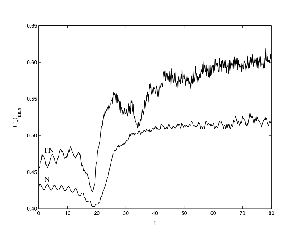
FIG. 5.: Evolution of the maximum density in the two coalescence calculations. The upper curve is for the PN run, the lower curve for the N run. The sharp decline in density at $t\simeq 15$ occurs as the two NS are tidally disrupted, followed by a larger increase as they coalesce.

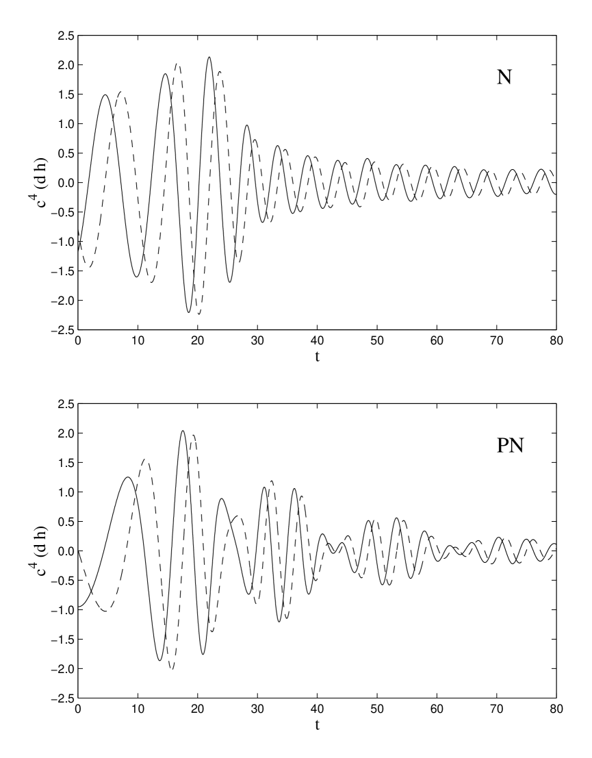
FIG. 6.: Gravity wave signatures for the two coalescence runs. The waveforms are calculated for an observer at a distance $d$ along the rotation axis. The solid line shows the $h_{+}$ polarization, the dashed line the $h_{\times}$ polarization (see Eqs. 23,24). At late times in the N run the waveforms show a simple, exponentially damped oscillation, whereas in the PN run an additional large-amplitude modulation is apparent.

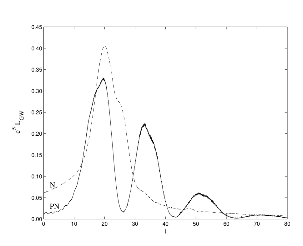
FIG. 7.: Gravity wave luminosity for the two coalescence runs (see Eq. 25). The solid line is for the PN run, the dashed line for the N run. The peak luminosity in the PN run is smaller than that of the N run, but secondary peaks occur at $t\simeq 35$, $50$, and $70$.

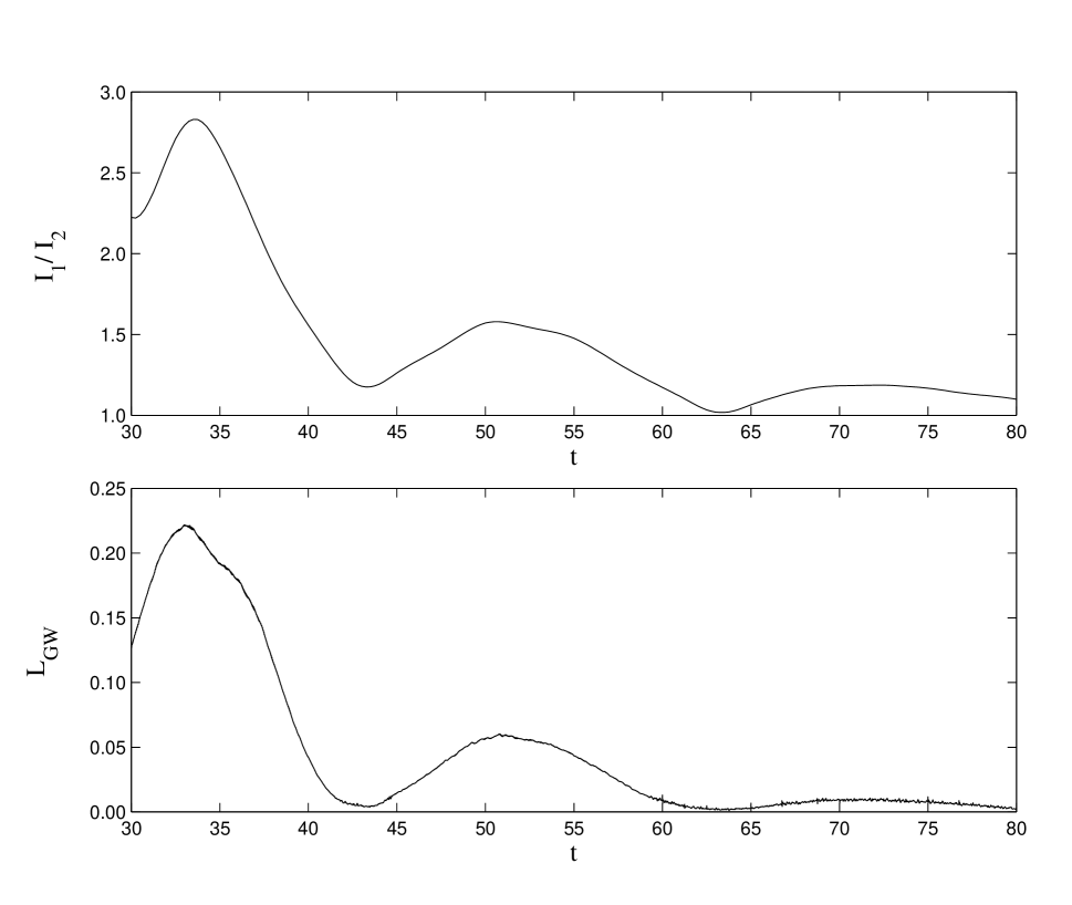
FIG. 8.: The ratio of the principal moments of inertia in the equatorial plane for the PN merger remnant, compared to the gravity wave luminosity at late times. The times of maximum elongation correspond to maxima in the gravity wave luminosity, and to decreases in the maximum density in Fig. 5 at $t\simeq 35$ and $t\simeq 50$ (and less clearly at $t\simeq 70$).

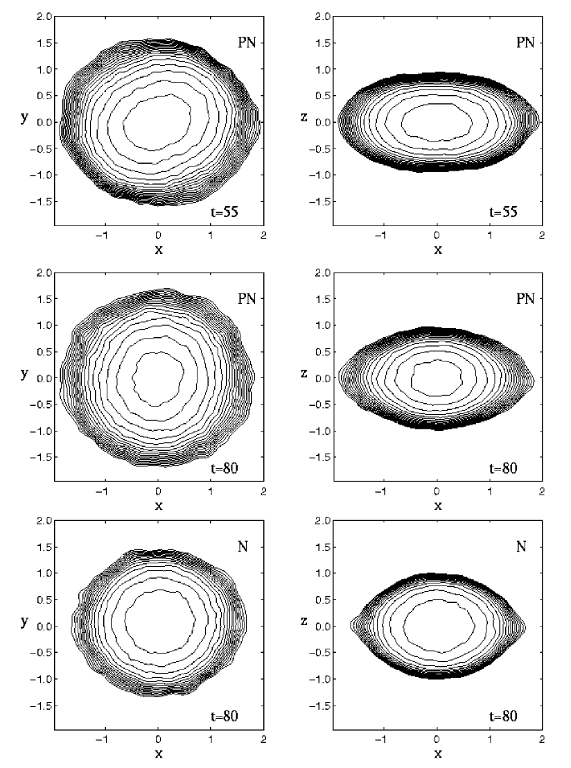
FIG. 9.: Density contours of the merger remnants. The top frames show the PN remnant at $t=55$, the middle ones show the same remnant at $t=80$, and the lower ones show the N remnant at $t=80$. The left frames show a cut through the equatorial plane, the right frames through the vertical plane (containing the rotation axis). Contours are logarithmic, ten per decade, starting from the maximum density of $(r_{*})_{max}=0.567$ for the PN run at $t=55$, $(r_{*})_{max}=0.608$ for the PN run at $t=80$, and $(r_{*})_{max}=0.518$ for the N run at $t=80$. The axes have been rotated to fall along the principal axes of the remnant. Note the cusp-like shape of the contours near the equator in the vertical plane, indicating maximal rotation.

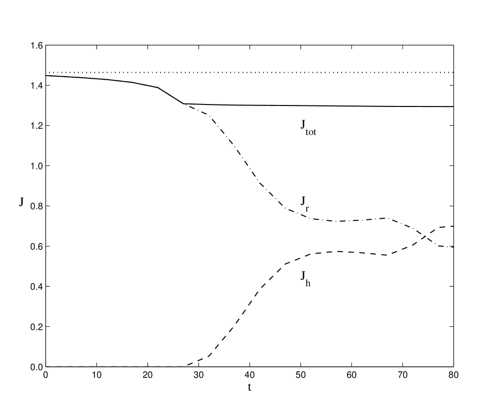
FIG. 10.: Evolution of the angular momentum in various components in the N run. Here $J_{tot}$ is the total angular momentum in the system, $J_{r}$ is for the inner remnant (defined by the condition $r_{*}>0.005$, which includes the entire binary initially, but only the inner remnant at later times), and $J_{h}$ is for the outer halo (so that $J_{tot}=J_{r}+J_{h}$). The dotted line shows the initial angular momentum of the system.

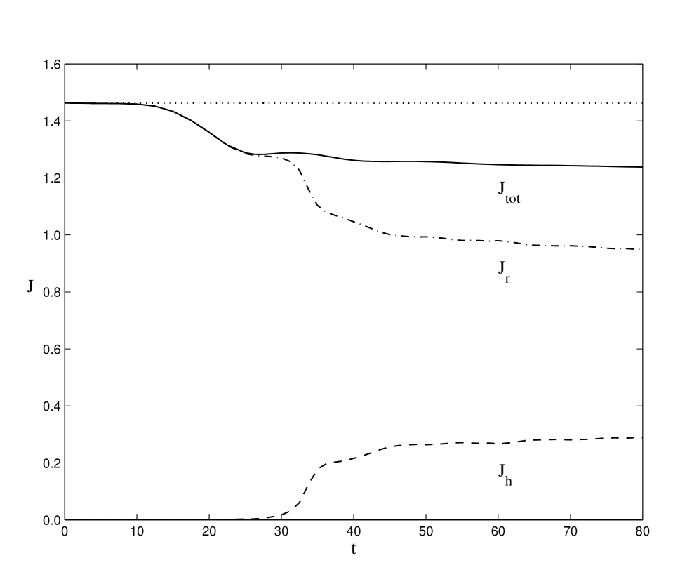
FIG. 11.: Evolution of the angular momentum in various components in the PN run. Conventions are as in Fig. 10.

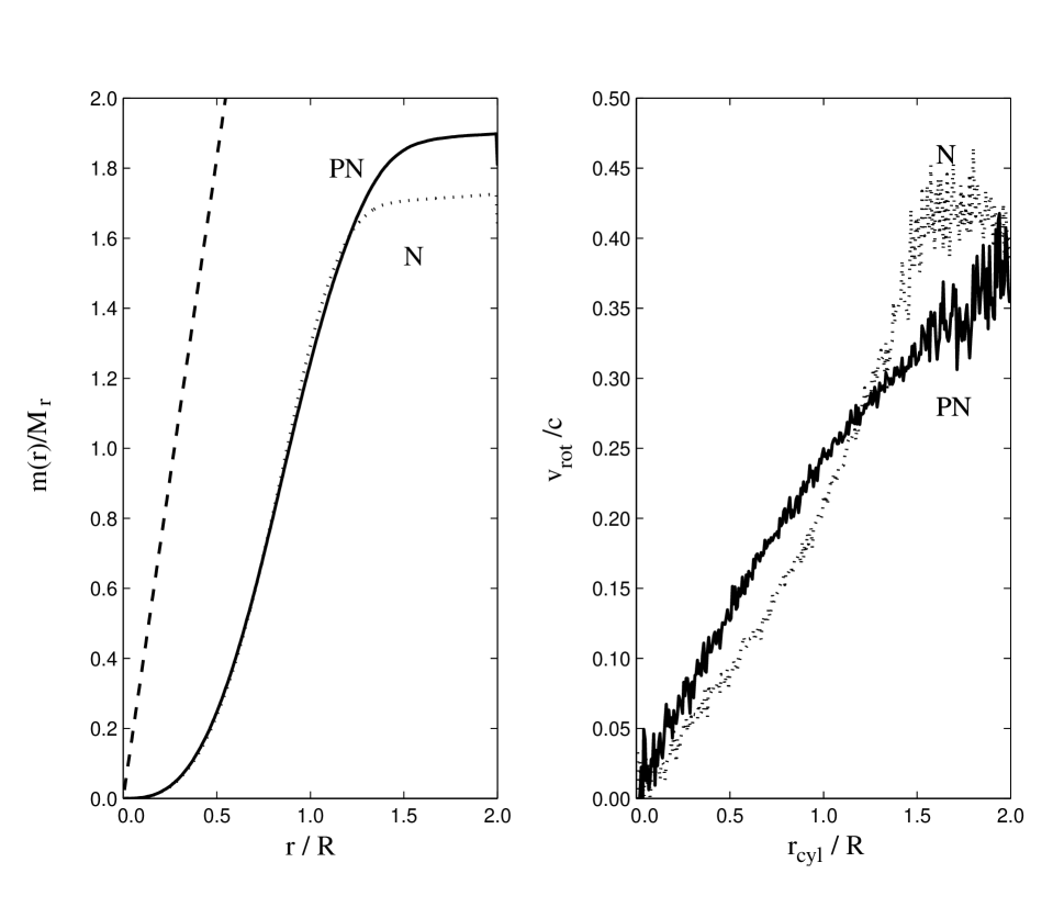
FIG. 12.: Enclosed rest mass and radially averaged rotational velocity profiles of the final merger remnant at t=80 for the two runs. Here, $r_{cyl}$ is the distance from the rotation axis, while $r$ is the radius from center. In both plots, the solid line is for the PN run, the dotted line for the N run. The dashed line shows the radius for a Kerr black hole with $a=0.7$ (the value we find for the PN run at t=80). For the rotational profile, we show only the data for $-0.1<z<0.1$, all other horizontal cuts yielding similar profiles extending to smaller radii.

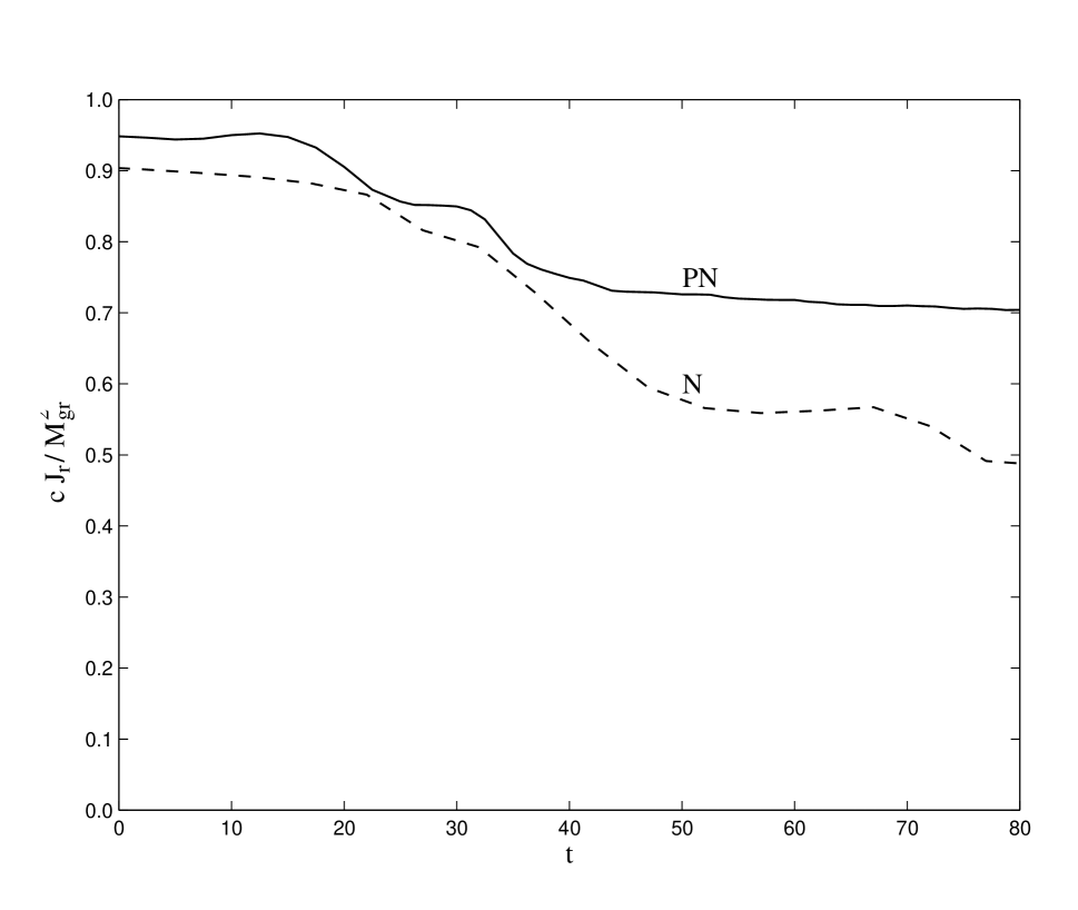
FIG. 13.: The evolution of the Kerr parameter $a_{r}\equiv cJ_{r}/M_{gr}^{2}$, for the inner remnant in the PN run (solid line) and in the N run (dashed line). At no time do we have $a_{r}>1$. The inner remnant (or core) is defined by the same density cut as in Fig. 10.

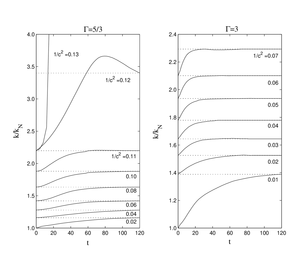
FIG. 14.: Results of SPH relaxation calculations for single stars. The ratio of the PN specific entropy $k$ to the Newtonian value $k_{N}$, is shown for both $\Gamma=5/3$ and $\Gamma=3$, computed for sequences of increasing compactness $1/c^{2}$. The dotted lines give the final value for each case, which was used as the initial value for the next relaxation. For $\Gamma=5/3$, we see that for $1/c^{2}>0.12$, $k/k_{N}$ increases without bounds, indicating instability. For $\Gamma=3$ and $1/c^{2}\gtrsim 0.07$, the 1PN approximation breaks down.

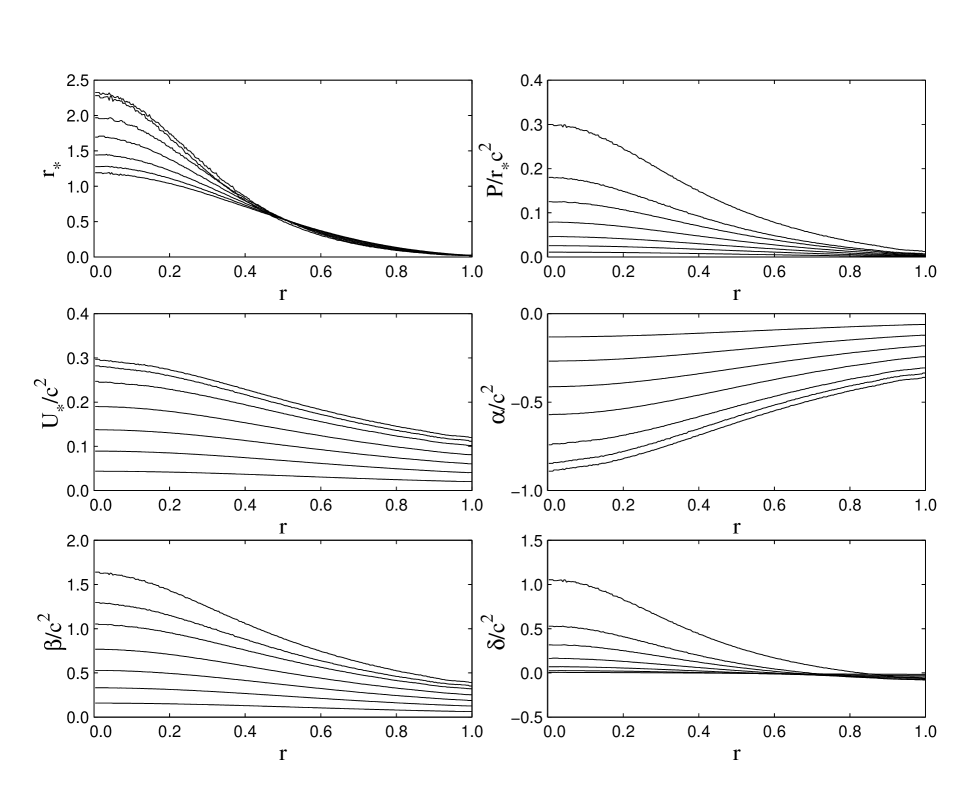
FIG. 15.: Radial profiles for the $\Gamma=5/3$ single star models. The various lines correspond, in monotonic fashion, to the stable configurations indicated by dotted lines in the left panel of Fig. 14.

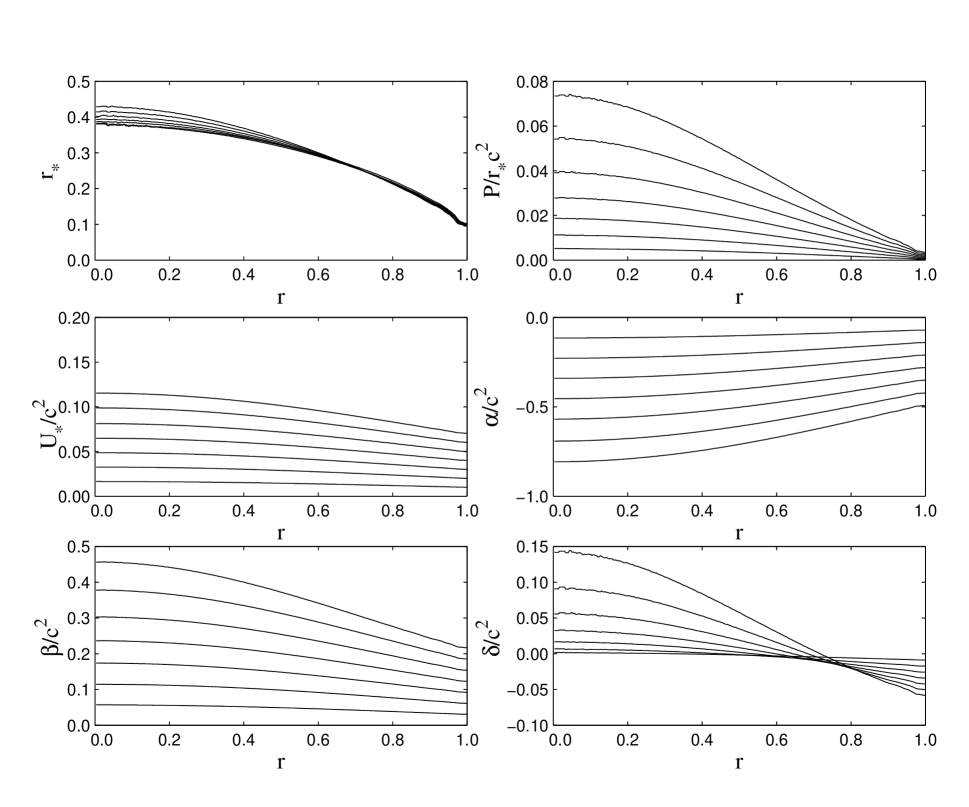
FIG. 16.: Radial profiles for the $\Gamma=3$ single star models. The lines correspond, in monotonic fashion, to the stable configurations indicated by dotted lines in the right panel of Fig. 14.

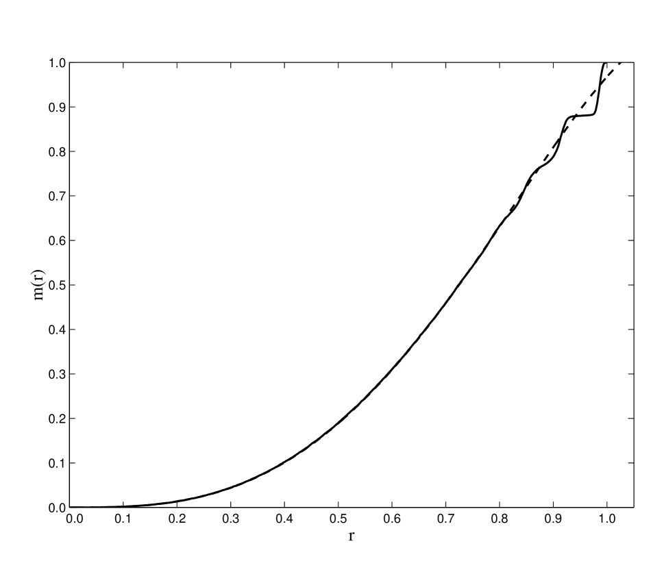
FIG. 17.: Mass profile of the $\Gamma=3$ single NS model with $1/c^{2}=0.05$, used in the PN run (solid), compared to a solution of Eqs. (B1–B10) obtained by a direct numerical integration (dashed). The agreement is excellent, except near the outer surface of the star, where the SPH density profile is more poorly defined.

TABLE I.: Properties of the Merger Remnants. Units are such that $G=M=R=1$, where $M$ and $R$ are the mass and radius of a single, spherical NS. Here, $M_{r}$ is the rest mass of the remnant, $M_{gr}$ is its gravitational mass, $J_{r}$ is its total angular momentum, $\Omega_{c}$ and $\Omega_{eq}$ are the angular rotation velocities at the center and at the equator, and the $a_{i}$’s and $I_{i}$’s are the principle axes and moments of inertia.

	$N(t=80)$	$PN(t=55)$	$PN(t=80)$
$M_{r}$	$1.73$	$1.90$	$1.89$
$M_{gr}$	$N/A$	$1.85$	$1.84$
$J_{r}$	$0.56$	$0.98$	$0.95$
$cJ_{r}/M_{gr}^{2}$	$0.47$	$0.72$	$0.70$
$\Omega_{c}$	$0.45$	$0.80$	$0.75$
$\Omega_{eq}$	$0.67$	$0.47$	$0.48$
$a_{1}$	$1.65$	$1.90$	$1.82$
$a_{2}$	$1.35$	$1.58$	$1.53$
$a_{3}$	$0.95$	$0.92$	$0.93$
$a_{2}/a_{1}$	$0.82$	$0.83$	$0.84$
$a_{3}/a_{1}$	$0.58$	$0.48$	$0.51$
$I_{1}$	$0.575$	$0.861$	$0.741$
$I_{2}$	$0.477$	$0.583$	$0.674$
$I_{3}$	$0.247$	$0.228$	$0.236$
$I_{2}/I_{1}$	$0.829$	$0.677$	$0.909$
$I_{3}/I_{1}$	$0.429$	$0.274$	$0.319$

TABLE II.: Parameters for Single Star Models. For each model, we list the compactness parameter $1/c^{2}$, the ratio of the PN specific entropy $k$ to the Newtonian value $k_{N}$, and the central values of density $r_{*}$, and the dimensionless ratios $P/r_{*}c^{2}$ and $U_{*}/c^{2}$.

$1/c^{2}$	$k/k_{N}$	$(r_{*})_{c}$	$(P/r_{*}c^{2})_{c}$	$(U_{*}/c^{2})_{c}$
		$\Gamma=5/3$
0.02	1.177	1.201	0.0111	0.0438
0.04	1.281	1.292	0.0257	0.0893
0.06	1.421	1.452	0.0464	0.1377
0.08	1.634	1.708	0.0792	0.1902
0.10	1.879	1.976	0.1255	0.2470
0.11	2.198	2.336	0.1806	0.2820
0.12	3.400	2.295	0.3011	0.2968
		$\Gamma=3$
0.01	1.403	0.3822	0.0052	0.0165
0.02	1.553	0.3818	0.0114	0.0326
0.03	1.649	0.3882	0.0187	0.0486
0.04	1.780	0.3948	0.0280	0.0649
0.05	1.918	0.4051	0.0397	0.0813
0.06	2.084	0.4170	0.0549	0.0989
0.07	2.262	0.4321	0.0746	0.1154

REFERENCES

- [1] M. Abramovici et al., Science 256, 325 (1992).
- [2] C. Bradaschia et al., Nucl. Instrum. Methods A289, 518 (1990).
- [3] J. Hough, in Proceedings of the Sixth Marcel Grossmann Meeting, edited by H. Sato and T. Nakamura (World Scientific, Singapore, 1992), p. 192.
- [4] K. Danzmann, in Relativistic Astrophysics, proceedings of the 162nd W.E. Heraeus Seminar, edited by H. Riffert et al. (Wiesbaden: Vieweg Verlag, 1998), p.48.
- [5] K. Kuroda et al., in Proceedings of the International Conference on Gravitational Waves: Sources and Detectors, edited by I. Ciufolini and F. Fidecard (World Scientific, 1997), p.100.
- [6] E.E. Flanagan and S.A. Hughes, Phys. Rev. D 57, 4566 (1998).
- [7] V.M. Lipunov, K.A. Postnov, and M.E. Prokhorov, Astrophys. L. 23, 492 (1997).
- [8] B.F. Schutz, Nature 323, 310 (1986); D.F. Chernoff and L.S. Finn, Astrophys. J. Lett. 411, L5 (1993); D. Marković, Phys. Rev. D 48, 4738 (1993).
- [9] V. Kalogera, in Proceedings of the Third Amaldi Conference on Gravitational Waves, edited by S. Meshkov (AIP Conference Series, to be published), astro-ph/9911532.
- [10] L.S. Finn and D.F. Chernoff, Phys. Rev. D 47, 2198 (1993).
- [11] R. Narayan, T. Piran, and A. Shemi, Astrophys. J. Lett. 379, L17 (1991); E.S. Phinney, ibid. 380, L17 (1991).
- [12] E.P.J. van den Heuvel and D.R. Lorimer, Mon. Not. R. Astron. Soc. 283, L37 (1996); I.H. Stairs et al., Astrophys. J. 505, 352 (1998).
- [13] S.J. Curran and D.R. Lorimer, Mon. Not. R. Astron. Soc. 276, 347 (1995).
- [14] Z. Arzoumanian, J.M. Cordes, and I. Wasserman, Astrophys. J. 520, 696 (1999).
- [15] V. Kalogera and D.R. Lorimer, Astrophys. J. (to be published), astro-ph/9907426.
- [16] W. Lincoln and C.M. Will, Phys. Rev. D 42, 1123 (1990); W. Junker and G. Schäfer, Mon. Not. R. Astron. Soc. 254, 146 (1992); C.M. Will, in Relativistic Cosmology, edited by M. Sasaki (Universal Academy Press, 1994), p.83; L.E. Kidder, C.M. Will, and A.G. Wiseman, Class. Quant. Grav. 9, L125 (1992); L. Blanchet, B.R. Iyer, C.M. Will, and A.G. Wiseman, ibid. 13, 575 (1996).
- [17] B.J. Meers, Phys. Rev. D 38, 2317 (1988); K.A. Strain and B.J. Meers, Phys. Rev. Lett. 66, 1391 (1991).
- [18] D. Eichler, M. Livio, T. Piran, and D.N. Schramm, Nature 340, 126 (1989); R. Narayan, B. Paczyński, and T. Piran, Astrophys. J. Lett. 395, L83 (1992); P. Mészáros, and M.J. Rees. 1992, Astrophys. J. 397, 570 (1992).
- [19] J.S. Bloom, S. Sigurdsson, and O.R. Pols, Mon. Not. R. Astron. Soc. 305, 763 (1999).
- [20] P. Mészáros, M.J. Rees, and R.A.M.J. Wijers, New Astron. 4, 303 (1999).
- [21] F.A. Rasio, in Black Holes in Binaries and Galactic Nuclei, edited by L. Kaper, E.P.J. van den Heuvel, and P.A. Woudt (in press, 2000).
- [22] F.A. Rasio and S.L. Shapiro, Astrophys. J. 401, 226 (1992) [RS1]; 432, 242 (1994) [RS2]; 438, 887 (1995) [RS3].
- [23] S. Chandrasekhar, Ellipsoidal Figures of Equilibrium; Revised Dover Edition (Yale University Press, New Haven, 1987).
- [24] D. Lai, F.A. Rasio, and S.L. Shapiro, Astrophys. J. Suppl. Ser. 88, 205 (1993) [LRS1]; Astrophys. J. Lett. 406, L63 (1993) [LRS2]; Astrophys. J. 420, 811 (1994) [LRS3]; 423, 344 (1994) [LRS4]; 437, 742 (1994) [LRS5].
- [25] T. Nakamura, in Relativistic Cosmology, edited by M. Sasaki (Universal Academy Press, 1994), p.155; T. Nakamura and K. Oohara, preprint [gr-qc/9812054].
- [26] K.C.B. New and J.E. Tohline, Astrophys. J. 490, 311 (1997).
- [27] F.D. Swesty, E.Y.M. Wang, and A.C. Calder, AStrophys. J. (to be published), astro-ph/9911192.
- [28] X. Zhuge, J. Centrella, and S. McMillan, Phys. Rev. D 50, 6247 (1994).
- [29] X. Zhuge, J. Centrella, and S. McMillan, Phys. Rev. D 54, 7261 (1996).
- [30] M.B. Davies, W. Benz, T. Piran, and F.K. Thielemann, Astrophys. J. 431, 742 (1994); M. Ruffert, H.-Th. Janka, K. Takahashi, and G. Schäfer, Astron. Astrophys. 319, 122 (1997).
- [31] M. Ruffert, H.-Th. Janka, and G. Schäfer, Astron. Astrophys. 311, 532 (1996).
- [32] M. Ruffert, M. Rampp, and H.-Th. Janka, Astron. Astrophys. 321, 991 (1997).
- [33] H.-Th. Janka, Th. Eberl, M. Ruffert, and C.L. Fryer, Astrophys. J. (to be published), astro-ph/9908290; S. Rosswog et al., Astron. Astrophys. 341, 499 (1999).
- [34] S.L. Shapiro, Phys. Rev. D 58, 3002 (1998).
- [35] D. Lai and A.G. Wiseman, Phys. Rev. D 54, 3958 (1997); M. Shibata and K. Taniguchi, ibid. 56, 811 (1997).
- [36] J.C. Lombardi, F.A. Rasio, and S.L. Shapiro, Phys. Rev. D 56, 3416 (1997).
- [37] T.W. Baumgarte et al., Phys. Rev. D 57, 7299 (1998).
- [38] P. Marronetti, G.J. Mathews, and J.R. Wilson, Phys. Rev. D 58, 7503 (1998); E.Y.M. Wang, F.D. Swesty, and A.C. Calder, in Proceedings of the Second Oak Ridge Symposium on Atomic and Nuclear Astrophysics, edited by A. Mezzacappa (Institute of Physics Publishing, 1998), p.723.
- [39] T.W. Baumgarte, S.A. Hughes, and S.L. Shapiro, Phys. Rev. D 60, 7501 (1999); W. Landry and S.A. Teukolsky, Phys. Rev. D (to be published), gr-qc/9912004; M. Miller, W. Suen, and M. Tobias, Phys. Rev. D (to be published), gr-qc/9910022; E. Seidel, in Relativistic Astrophysics, proceedings of the 162nd W.E. Heraeus Seminar, edited by H. Riffert et al. (Wiesbaden: Vieweg Verlag, 1998), p.229; M. Shibata, Phys. Rev. D 60, 4052 (1999).
- [40] M. Shibata and K. Uryu, Phys. Rev. D (to be publshed), gr-qc/9911058.
- [41] K. Taniguchi and M. Shibata, Phys. Rev. D 56, 798 (1997); K. Taniguchi, Prog. Theor. Phys. 101, 283 (1999).
- [42] A. Buonanno and T. Damour, Phys. Rev. D 59, 4006 (1999).
- [43] G. Schäfer, in Proceedings of the Fifth Marcel Grossman Meeting, edited by D.G. Blair and M.J. Buckingham (World Scientific, Singapore, 1989).
- [44] L. Blanchet, T. Damour, and G. Schäfer, Mon, Not. R. Astron. Soc. 242, 289 (1992) [BDS].
- [45] M. Shibata, K. Oohara, and T. Nakamura. Prog. Theor. Phys. 98, 1081 (1997).
- [46] S. Ayal et al., Astrophys. J. (submitted), astro-ph/9910154.
- [47] A. Akmal, V.R. Pandharipande, and D.G. Ravenhall, Phys. Rev. C 58, 1804 (1998).
- [48] J.C.L. Wang et al., Astron. Astrophys. 345, 869 (1999).
- [49] R. Dave, J. Dubinsky, and L. Hernquist, New Astron. 2, 277 (1997); F.A. Rasio, in Proceedings of the 5th International Conference on Computational Physics (ICCP5), (to be published, 2000).
- [50] L.B. Lucy, Astron. J. 82, 1013 (1977); R.A. Gingold and J.J. Monaghan, Astrophys. J. 181, 375 (1977).
- [51] J.J. Monaghan, Ann. Rev. Astron. Astrophys. 30, 543 (1992).
- [52] F.A. Rasio and S.L. Shapiro, Astrophys. J. 377, 559 (1991).
- [53] M. Frigo and S. Johnson, MIT Laboratory of Computer Science Publication MIT-LCS-TR-728, 1997; the code is freely available at http://www.fftw.org.
- [54] J.C. Lombardi, A. Sills, F.A. Rasio, and S.L. Shapiro, J. Comput. Phys. 152, 687 (1999).
- [55] D. Balsara, J. Comput. Phys. 121, 357 (1995).
- [56] S.L. Shapiro and S. Teukolsky, Black Holes, White Dwarfs, and Neutron Stars (Wiley, New York, 1983).
- [57] J.-P. Zahn, in Binaries as Tracers of Stellar Formation, edited by A. Duquennoy and M. Mayor (Cambridge, Cambridge University Press, 1992), p. 253.
- [58] C. Del Noce, G. Preti, and F. de Felice, Astrophys. J. 507, 287 (1998); T.W. Baumgarte, S.L. Shapiro, and M. Shibata, Astrophys. J. Lett. 528, L29 (2000).
- [59] R.B. Wiringa, V. Fiks, and A. Fabrocini, Phys. Rev. C 38, 1010 (1988).
- [60] G.B. Cook, S.L. Shapiro, and S.L. Teukolsky, Astrophys. J. 424, 823 (1994).
- [61] D. Lai and S.L. Shapiro, Astrophys. J. 442, 259 (1995).
- [62] T.W. Baumgarte and S.L. Shapiro, Astrophys. J. 504, 431 (1998).
- [63] J.M. Lattimer and D. Swesty, Nucl. Phys. A535, 331 (1991).
- [64] G. Baym, in Neutron Stars: Theory and Observation, edited by J. Ventura and D. Pines (Dordrecht, Kluwer, 1991), p. 21.
- [65] M. van Kerkwijk, personal communication.
- [66] S.E. Thorsett and D. Chakrabarty, D., Astrophys. J. 512, 288 (1999).
- [67] J.H. Taylor and J.M. Weisberg, Astrophys. J. 345, 434 (1989).
- [68] C.S. Kochanek, Astrophys. J. 398, 234 (1992); L. Bildsten and C. Cutler, ibid. 400, 175 (1992).
- [69] F.A. Rasio and S.L. Shapiro, Class. Quant. Grav. 16, 1 (1999).