Non-minimally coupled scalar fields in homogeneous universes

Abstract

The equations governing the evolution of non-minimally coupled scalar matter and the scale factor of a Robertson-Walker universe are derived from a minisuperspace action. As for the minimally coupled case, it is shown that the entire semiclassical dynamics can be retrieved from the Wheeler-DeWitt equation via the Born-Oppenheimer reduction, which properly yields the (time-time component of the) covariantly conserved energy-momentum tensor of the scalar field as the source term for gravity. However, for a generic coupling, the expectation value of the operator which evolves the matter state in time is not equal to the source term in the semiclassical Einstein equation for the scale factor of the universe and the difference between these two quantities is related to the squeezing and quantum fluctuations of the matter state. We also argue that matter quantum fluctuations become relevant in an intermediate regime between quantum gravity and semiclassical gravity and study several cases in detail.

I Introduction

Non-minimally coupled scalar fields have been extensively used in the literature to account for higher loop quantum corrections to the theory of scalar fields in the general relativity theory of gravitation (see, e.g., [1] and Refs. therein). However, contrary to the minimally coupled case, quantization of such fields in the framework of quantum field theories on a classical curved background makes an ambiguity apparent. In fact, there appear a boundary term in the action for the scalar field which arises when using rescaled fields and whose presence changes the canonical matter Hamiltonian [2]. Thus, depending on whether one retains or drops such a term yields apparently different Schrödinger equations for the state of the scalar field [3].

This ambiguity can be understood by noting that, classically, the above mentioned boundary term is generated because the rescaling of the scalar field by a function of the scale factor of the universe is a time dependent canonical transformation [4]. Therefore, in the quantum theory, it is associated with a (possibly unitary) transformation between different Fock spaces (choices of the ground state for matter). The ambiguity can then be eliminated [3] by introducing the invariant Fock space built upon invariant operators [5] which are not affected by a boundary term added to the action. However, since the matter energy (the time-time component of the energy-momentum tensor) is related to the matter Hamiltonian, the interpretation in terms of particle content (or gravitational “weight”) of a quantum state of matter remains an open question.

The latter is not an academic issue, since, classically, it is the matter energy which acts as a source for gravity in the Einstein equations and determines the history of the universe. Hence, it is of primary concern to clarify by means of which quantity a quantized state of matter drives the metric at the semiclassical level. In order to do so, we appeal to the principle that time-reparameterization invariance is a fundamental property of any gravitational system which also generates the dynamics and be lifted to a quantum symmetry. Then, one expects to have an Hamiltonian constraint from which the Born-Oppenheimer (BO) reduction [6, 7, 8] allows to properly and unambiguously recover the semiclassical limit starting from the Wheeler-DeWitt (WDW) equation [9, 10].

The above scheme has proven remarkably successful for the minimally coupled scalar field in Robertson-Walker space-time [11]. In that case one starts with an action $S=S(N,a,\phi)$ for the three minisuperspace variables $N$ (lapse function), $a$ (scale factor) and $\phi$ (one mode of a scalar field) which are functions of an arbitrary time $t$. Upon varying $S$ one obtains three Euler-Lagrange equations of motion (for the details, see next Sections and, e.g., Ref. [8])

$${\delta S\over\delta N}\equiv-H=0\ \ \ \ \ \ \ \ \ \hbox{(Hamiltonian\ constraint)}$$ (1)

$${\delta S\over\delta a}=0$$ (2)

$${\delta S\over\delta\phi}=0\ \ \ \ \ \ \ \ \ \ \ \ \ \ \ \ \ \ \ \hbox{(Klein-Gordon\ equation)}\ .$$ (3)

Since Eq. (1) is a constraint, $N=N(t)$ is arbitrary and one can set, e.g., $N(t)=1$ for $t_{i}\leq t\leq t_{f}$ (proper time gauge) provided the initial conditions $a(t_{i})$, $\dot{a}(t_{i})$, $\phi(t_{i})$ and $\dot{\phi}(t_{i})$ are such that $H(t_{i})=0$ (an overdot denotes the derivative with respect to $t$). Then Eqs. (2) and (3) will evolve the initial data to any time $t_{i}<t\leq t_{f}$ consistently, since

$$\left\{\begin{array}[]{l}\displaystyle{\delta S\over\delta a}=0\\ \\ \displaystyle{\delta S\over\delta\phi}=0\end{array}\right.\ \ \Rightarrow\ \ {dH\over dt}=0\ ,$$ (7)

which proves that the Hamiltonian constraint is preserved by the dynamics. However, for practical purposes it is more convenient to revert the above inference and observe that the equation of motion (2) for $a$ is identically satisfied provided the Hamiltonian constraint (1) is enforced at all times along with the Klein-Gordon equation (3),

$$\left\{\begin{array}[]{l}\displaystyle H(t)=0\\ \phantom{H(t)=0}\ \ \ (t_{i}\leq t\leq t_{f})\\ \displaystyle{\delta S\over\delta\phi}=0\end{array}\right.\ \ \Rightarrow\ \ {\delta S\over\delta a}=0\ .$$ (11)

A further simplification is then obtained at the semiclassical level, where one can show that both the Hamiltonian constraint and the Klein-Gordon equation follow from the WDW equation obtained by quantizing the super-Hamiltonian $H$,

$$\hat{H}\,\Psi\equiv\left(\hat{H}_{G}+\hat{H}_{M}\right)\,\Psi=0\ ,$$ (12)

where $H_{G}$ and $H_{M}$ are respectively referred to as the gravitational and matter Hamiltonian. In fact, the BO decomposition for the wavefunction of the universe,

$$\Psi(a,\phi)=\psi(a)\,\chi(\phi,a)\ ,$$ (13)

leads to the coupled equations

$$H_{G}+\mbox{$\langle\,\hat{H}_{M}\,\rangle$}=0\ \ \ \ \ \ \ \ \ \hbox{(Einstein-Hamilton-Jacobi\ equation)}$$ (14)

(15)

$$i\,\hbar\,{\partial\chi_{s}\over\partial t}=\hat{H}_{M}\,\chi_{s}\ \ \ \ \ \ \ \ \ \hbox{(Schr\"{o}dinger\ equation)}\ ,$$ (16)

along with explicit conditions on the wavefunctions $\psi$ and $\chi$ for the validity of such an approximation. We then note that Eq. (14) is the semiclassical analogue of Eq. (1) and the operator $\hat{H}_{M}$ in Eq. (16) evolves in time states $\chi_{s}$ of the scalar field in such a way that the expectation value of $\hat{\phi}$ over coherent states satisfies the Klein-Gordon equation (3). If one regards coherent states as being the quantum states which are closest to classical, one can conclude that the entire semiclassical dynamics is encoded in the single WDW equation (12) and is properly retrieved by the BO reduction.

We wish to remark here the fact that the decomposition (13) is not related to the gravitational scale of mass being bigger than any matter scale, therefore Eqs. (14) and (16) do not require an expansion in powers of the Planck mass [12] (see also [8], where such an expansion is shown to violate unitarity when incorrectly performed). Indeed, the relevant ratio is between the energy of each quantum of $\phi$ and the total energy of such quanta. This can be understood if one considers that the scale factor of the universe is a collective variable associated with the total energy of matter in space and that such an energy is presently much bigger than the energy of each of its microscopic constituents (described by the degree of freedom $\phi$). Basically, this fact, the huge amount of matter particles, is the reason we live in a semiclassical universe [9]. Consequently, one expects a failure in the semiclassical approximation which leads to Eqs. (14) and (16) for matter states $\chi$ containing a small number of quanta. In fact, this expectation has been systematically verified in all the cases studied so far [13, 14, 15, 16].

When one applies the same scheme to the non-minimally coupled case, a new ambiguity arises because then there is no clear way of splitting the action into a matter part and a gravitational part and a preferred classical form for the energy-momentum tensor of the scalar field can indeed be singled out only by requiring covariant conservation [17]. Correspondingly, one could write many (classically equivalent) Hamiltonian constraints which, at the quantum level, become inequivalent “WDW” equations. Interestingly, the BO factorization (13) pinpoints a specific form of (or operator ordering in) the WDW equation in order to ensure the existence of the Schrödinger equation (16). Further, the BO reduction then yields a source term for the geometry in the semiclassical Einstein equation (14) which can be easily related to the time-time component of the proper (divergenceless) energy-momentum tensor of the scalar field. However, such a source is not equal to the expectation value of the Hamiltonian operator in Eq. (16). It is only for the case of minimal coupling that the super-Hamiltonian is the sum of the time-time components of the (covariantly conserved) energy-momentum tensor and Einstein tensor and then the expectation value of the generator of the time evolution for the matter state is the semiclassical source of gravity.

In the following, we shall argue that the difference between the source term in the semiclassical Einstein equation and the operator of time-evolution in the Schrödinger equation is associated with the different ways matter and gravity are affected by quantum fluctuations around the mean value of the matter field and by the presence of a squeezing [18] term in the Schrödinger equation. This will lead us to define three different regimes of approximations, namely quantum gravity, semiclassical gravity and an “intermediate” regime in which quantum gravitational fluctuations are negligible but the trajectory of the (collective) gravitational degree of freedom senses matter fluctuations. Similar results were found previously in different approaches and, for example, the intermediate regime is called stochastic gravity by Hu and collaborators (for a review see e.g., [19] and Refs. therein).

The approach employed in the present paper might look totally different with respect to the procedure of estimating the back-reaction within the framework of quantum field theory by studying perturbations of the Einstein equations (or in the Feynman path integral) around a given classical solution [20]. It has certainly the shortcoming that we start from an effective minisuperspace action in which the degrees of freedom of the system have been reduced by symmetry arguments prior to quantization and subsequent semiclassical approximation, rather than from the quantized set of equations derived from the full Einstein-Hilbert action. However, we point out that the more standard approach of perturbation theory also reduces the degrees of freedom of Einstein gravity [21], since it assumes the existence of a classical (saddle point) solution (background manifold and metric) from the onset, leaving as remnant gauge freedom only coordinate transformations and small diffeomorphisms of the background manifold [20]. Both approaches are thus questionable if one wishes to quantize Einstein gravity, but can be regarded as hopefully reliable whenever one aims at describing gravity in a semiclassical state as we wish to do here.

In the following Section we start from the minisuperspace action for a mode of a non-minimally coupled massive scalar field in a Robertson-Walker space-time and pursue the standard canonical formalism in order to obtain an Hamiltonian constraint and the corresponding WDW equation. Then in Section III we apply the BO approach and obtain the Hamilton-Jacobi equation for the scale factor of the universe and the Schrödinger equation for the state of the scalar field. By making use of invariant operators we solve the Schrödinger equation and show that the source term in the semiclassical Einstein equation is the semiclassical extension of the time-time component of the covariantly conserved energy-momentum tensor. In Section IV we specialize the results to the massive minimally coupled case, which we briefly review, and to the particular cases with $\xi=1/6$ and $1/4$ which we analyze in more detail. Finally, in Section V we summarize and comment on our results.

We follow the sign convention of Ref. [11] and define $\kappa=8\,\pi\,G$.

II Minisuperspace action

In this Section we shall show that the classical dynamics of a non-minimally coupled scalar field in Robertson-Walker space-time is determined by the Hamiltonian constraint and the Klein-Gordon equation, thus generalizing the result (7) for the minimally coupled case as described in the Introduction.

The (volume part of the) action for the non-minimally coupled real scalar field $\Phi=\Phi(x)$ in a generic four-dimensional space-time ${\cal M}$ with metric $g$ is given by [1, 22]

$$S_{\Phi}={1\over 2}\,\int_{\cal M}d^{4}x\,\sqrt{-g}\,\left[R\,\left({1\over\kappa}-\xi\,\Phi^{2}\right)-\left(\partial\Phi\right)^{2}-\mu^{2}\,\Phi^{2}\right]\ ,$$ (17)

where $g=\det{\mbox{\boldmath$g$}}$, $R$ is the scalar curvature, $\mu=1/\ell_{\phi}$ the inverse of the Compton wavelength of $\Phi$ and $\xi$ a dimensionless parameter such that $\xi=0$ corresponds to the minimal coupling and $\xi=1/6$ yields the conformal coupling [23].

It is possible to reduce the above action by assuming spatial homogeneity and isotropy so that ${\cal M}$ admits a preferred foliation into spatial hypersurfaces of constant time $t$ and the four-metric is given by the Robertson-Walker line element [11]

$$ds^{2}=-N^{2}\,dt^{2}+a^{2}\,\left[{dr^{2}\over 1-k\,r^{2}}+r^{2}\,\left(d\theta^{2}+\sin^{2}\theta\,d\varphi^{2}\right)\right]\ ,$$ (18)

with $k=0,\pm 1$ for flat, positive and negative spatial curvature, $\theta$ and $\varphi$ the usual angular coordinates and $r\in[0,r_{k})$ with $r_{+1}=1$, $r_{0}=r_{-1}=+\infty$. The scalar curvature is then given by

$$R={6\over N^{2}}\,\left({\ddot{a}\over a}-{\dot{a}\,\dot{N}\over a\,N}+{\dot{a}^{2}\over a^{2}}+N^{2}\,{k\over a^{2}}\right)\ .$$ (19)

We also expand the real scalar field in spatial Fourier modes,

$$\Phi={1\over\sqrt{2\,V}}\,\sum_{\vec{p}}\,\left[e^{-i\,\vec{p}\cdot\vec{x}}\,\Phi_{\vec{p}}+e^{i\,\vec{p}\cdot\vec{x}}\,\Phi^{\star}_{\vec{p}}\right]\ ,$$ (20)

where ${\cal V}=a^{3}\,V$ is the spatial volume of the universe, and separate the real from the imaginary part,

$$\Phi_{\vec{p}}(t)={1\over\sqrt{2}}\,\left(\phi_{\vec{p}}^{1}+i\,\phi_{\vec{p}}^{2}\right)\ .$$ (21)

This decomposition yields an effective action for two minisuperspace variables $a=a(t)$ and $\phi=\phi(t)$ (for the details see Appendix A),

$$S={1\over 2}\,\int_{t_{i}}^{t_{f}}dt\,\left\{a^{3}\,\left({\dot{\phi}^{2}\over N}-N\,\omega^{2}\,\phi^{2}\right)+6\,\left(v-\xi\,\phi^{2}\right)\,\left[{a\,\dot{a}^{2}\over N}+N\,k\,a+a^{2}\,{d\over dt}\left({\dot{a}\over N}\right)\right]\right\}\ ,$$ (22)

where $v\equiv V/\kappa$. The action $S$ can be used to analyze (the real or imaginary part of) any of the modes $\Phi_{\vec{p}}$, with an effective frequency $\omega$ as given in Eq. (A13).

The above action contains both a second time derivative of $a$ and a first time derivative of $N$ in the same term. The former would cause problems with causality and requires a modification of the standard Euler-Lagrange equations of motion; the latter breaks the presumed time-reparameterization invariance of the system. However, we observe that upon integrating by parts the last term and neglecting the integrated part as dynamically irrelevant (for further explanation see Appendix B), one finally obtains

$$S={1\over 2}\,\int_{t_{i}}^{t_{f}}N\,dt\,a^{3}\,\left[{\dot{\phi}^{2}\over N^{2}}-\omega^{2}\,\phi^{2}-{6\over a^{2}}\,\left(v-\xi\,\phi^{2}\right)\,\left({\dot{a}^{2}\over N^{2}}-k\right)+12\,\xi\,{\phi\over a}\,{\dot{a}\,\dot{\phi}\over N^{2}}\right]\ ,$$ (23)

in which there are no second time derivatives and $d\tau\equiv N\,dt$ is the proper time measure. This is the action we regard as properly describing the dynamics of the coupled variables $a$ and $\phi$.

A Lagrangean dynamics

The Euler-Lagrange equations of motion following from the action $S$ are given by

$${1\over a^{3}}\,{\delta S\over\delta N} \equiv -{H\over a^{3}}$$ (24)

$$= 3\,\left(v-\xi\,\phi^{2}\right)\,\left({\dot{a}^{2}\over a^{2}}+{k\over a^{2}}\right)-{1\over 2}\,\left(\dot{\phi}^{2}+\omega^{2}\,\phi^{2}\right)-6\,\xi\,{\dot{a}\over a}\,\phi\,\dot{\phi}=0$$ (25)

$${1\over a^{2}}\,{\delta S\over\delta a} = 3\,\left[\left(v-\xi\,\phi^{2}\right)\,\left(2\,{\ddot{a}\over a}+{\dot{a}^{2}\over a^{2}}+{k\over a^{2}}\right)-4\,\xi\,{\dot{a}\over a}\,\phi\,\dot{\phi}-2\,\xi\,\left(\dot{\phi}^{2}+\phi\,\ddot{\phi}\right)\right.$$ (28)

$$\phantom{3\,[}\left.+{1\over 2}\,\left(\dot{\phi}^{2}-\omega^{2}\,\phi^{2}\right)+2\,{\omega\over a^{2}}\,\vec{P}\cdot\vec{P}\,\phi^{2}\right]=0$$

$${1\over a^{3}}\,{\delta S\over\delta\phi} = -\left[\ddot{\phi}+3\,{\dot{a}\over a}\,\dot{\phi}+\omega^{2}\,\phi+6\,\xi\,\left({\ddot{a}\over a}+{\dot{a}^{2}\over a^{2}}+{k\over a^{2}}\right)\,\phi\right]=0\ ,$$ (30)

where we have set $N=1$ after the variation to give the expressions a simple form. This choice is consistent with the fact that the action (23) does not contain time derivatives of $N$ and Eq. (25) is then the Hamiltonian constraint. Of course it must be preserved in time and, in fact,

$${dH\over d\tau} = -3\,\dot{a}\,\left(v-\xi\,\phi^{2}\right)\,\left(\dot{a}^{2}+2\,a\,\ddot{a}+k\right)+{3\over 2}\,a^{2}\,\dot{a}\,\left(\dot{\phi}^{2}+\omega^{2}\,\phi^{2}\right)+a^{3}\,\dot{\phi}\,\left(\ddot{\phi}+\omega^{2}\,\phi\right)$$ (32)

$$+6\,\xi\,a\,\phi\,\dot{\phi}\,\left(3\,\dot{a}^{2}+k\right)+6\,\xi\,a^{2}\,\left(\dot{a}\,\dot{\phi}^{2}+\phi\,\ddot{a}\,\dot{\phi}+\phi\,\dot{a}\,\ddot{\phi}\right)-2\,\omega\,\vec{P}\cdot\vec{P}\,\dot{a}\,\phi^{2}$$

$$= -\dot{a}\,{\delta S\over\delta a}-\dot{\phi}\,{\delta S\over\delta\phi}$$ (33)

vanishes identically by virtue of Eqs. (28) and (30), thus generalizing to arbitrary $\xi$ the results (7) and (11) valid for $\xi=0$.

The next step is to quantize the system and show that the WDW equation encodes the entire semiclassical dynamics. In order to do so, one needs to consider the Hamiltonian form of Eq. (25).

B Hamiltonian dynamics

The canonical momenta conjugated to $N$, $a$ and $\phi$ are given by

$$P_{N}=0$$ (34)

(35)

$$P_{a}=-6\,a\,\left(v-\xi\,\phi^{2}\right)\,{\dot{a}\over N}+6\,\xi\,a^{2}\,\phi\,{\dot{\phi}\over N}$$ (36)

(37)

$$P_{\phi}=a^{3}\,{\dot{\phi}\over N}+6\,\xi\,a^{2}\,\phi\,{\dot{a}\over N}\ .$$ (38)

The action (23) can then be written in canonical form as

$$S=\int_{t_{i}}^{t_{f}}dt\,\left[P_{N}\,\dot{N}+P_{a}\,\dot{a}+P_{\phi}\,\dot{\phi}-N\,H(P_{a},P_{\phi},a,\phi)\right]\ ,$$ (39)

where the super-Hamiltonian already given in Eq. (25) takes on the rather complicated canonical form

$$H={1\over 2}\,\left\{-{\left[a\,P_{a}-6\,\xi\,\phi\,P_{\phi}\right]^{2}\over 6\,a^{3}\,\left[v-\xi\,\left(1-6\,\xi\right)\,\phi^{2}\right]}\,-6\,k\,a\,\left(v-\xi\,\phi^{2}\right)+{P_{\phi}^{2}\over a^{3}}+a^{3}\,\omega^{2}\,\phi^{2}\right\}\ .$$ (40)

Several remarks are in order. First, the cases $\xi=0$,

$$H={1\over 2}\,\left\{-{P_{a}^{2}\over 6\,v\,a}-6\,k\,v\,a+{P_{\phi}^{2}\over a^{3}}+\,a^{3}\,\omega^{2}\,\phi^{2}\right\}\ ,$$ (41)

and $\xi=1/6$,

$$H={1\over 2}\,\left\{-{\left(a\,P_{a}-\phi\,P_{\phi}\right)^{2}\over 6\,v\,a^{3}}-6\,k\,v\,a+{P_{\phi}^{2}\over a^{3}}+a\,\left(a^{2}\,\omega^{2}+k\right)\,\phi^{2}\right\}\ ,$$ (42)

are clearly special since these values of $\xi$ simplify the form of the kinetic term in $H$, although it is only for $\xi=0$ that the kinetic term is diagonal in the momenta [24].

Second, the $\tau\tau$-component of the unique divergenceless energy-momentum tensor as computed according to Ref. [17],

$$T_{\tau\tau}={1\over v-\xi\,\phi^{2}}\,\left[{1\over 2}\,\left(\dot{\phi}^{2}+\omega^{2}\,\phi^{2}\right)+6\,\xi\,{\dot{a}\over a}\,\phi\,\dot{\phi}\right]\ ,$$ (43)

is related to the variation of the action with respect to the metric by

$${2\over\sqrt{-g}}\,{\delta S_{M}\over\delta g^{\tau\tau}}=\left(v-\xi\,\phi^{2}\right)\,T_{\tau\tau}\ ,$$ (44)

where

$$S_{M}=-{1\over 2}\,\int d^{4}x\,\sqrt{-g}\,\left[\left(\partial\Phi\right)^{2}+\mu^{2}\,\Phi^{2}+\xi\,R\,\Phi^{2}\right]\ .$$ (45)

It is however the (non-conserved) quantity in the right hand side (r.h.s.) of Eq. (44) which naturally appears inside $H$, as is apparent from Eq. (25) or

$${H\over a^{3}} = \left(v-\xi\,\phi^{2}\right)\,\left[T_{\tau\tau}-3\,\left({\dot{a}^{2}\over a^{2}}+{k\over a^{2}}\right)\right]$$ (46)

$$= \left(v-\xi\,\phi^{2}\right)\,\left(T_{\tau\tau}-{1\over\kappa}\,G_{\tau\tau}\right)$$ (47)

$$\equiv \left(v-\xi\,\phi^{2}\right)\,{H^{\prime}\over a^{3}}\ ,$$ (48)

where $G_{\tau\tau}$ is the $\tau\tau$-component of the standard Einstein tensor. From Eq. (33) one concludes that

$${dH^{\prime}\over d\tau}\sim\phi\,\dot{\phi}\,H^{\prime}\ ,$$ (49)

therefore $G_{\tau\tau}=\kappa\,T_{\tau\tau}$, or $H^{\prime}=0$, is an equivalent statement of time-reparameterization invariance (assuming $v\not=\xi\,\phi^{2}$).

In order to lift such a symmetry to the quantum level and obtain the WDW equation one might choose either $H$ or $H^{\prime}$ (or any other classically equivalent expression), thus obtaining quantum mechanically inequivalent “WDW” equations. However, the existence of the semiclassical limit via the BO reduction places some restrictions on the form of the Hamiltonian constraint. In particular, in order to recover a Schrödinger equation from the WDW equation, it is necessary that the coefficient of $P_{a}^{2}$ does not depend on the matter degree of freedom $\phi$ (see Section III B for more details). This singles out the preferred (classical) expression

$$\bar{H} = W_{\xi}\,H$$ (50)

$$= {1\over 2}\,\left\{-{\left[a\,P_{a}-6\,\xi\,\phi\,P_{\phi}\right]^{2}\over 6\,a^{3}}+W_{\xi}\,\left[{P_{\phi}^{2}\over a^{3}}+a^{3}\,\omega^{2}\,\phi^{2}-6\,k\,a\,\left(v-\xi\,\phi^{2}\right)\,\right]\right\}\ ,$$ (51)

where $W_{\xi}=W_{\xi}(\phi)\equiv v-\xi\,\left(1-6\,\xi\right)\,\phi^{2}$.

We proceed to analyze the quantum version of the Hamiltonian constraint with the modified super-Hamiltonian (51) in the next Section where we shall also show that the BO approach guarantees that the metric be driven by the proper (conserved) semiclassical ($\tau\tau$-component of the) energy momentum tensor for the scalar field.

III Semiclassical equations

The quantization of the Hamiltonian constraint $\bar{H}=0$, with $\bar{H}$ as given in Eq. (51), is formally achieved by introducing the operators $\hat{a}$, $\hat{\phi}$, $\hat{P}_{a}$ and $\hat{P}_{\phi}$ which yields the WDW equation

$$\bar{H}(\hat{P}_{a},\hat{P}_{\phi},\hat{a},\hat{\phi})\,\Psi=0\ ,$$ (52)

where $\Psi=\Psi(a,\phi)$ is the wavefunction of the universe.

When dealing with Eq. (52) as it stands, one has to face several formal problems. First of all one would like to describe the system by means of Dirac variables, but, obviously, this is not the case for $a$ and $\phi$ and their momenta which do not commute with $\bar{H}$. This problem could be solved by trading the original canonical variables for their initial values (the so called perennials; for a review see Ref. [25]). Then one wishes the canonical variables map into Hermitian operators and, further, needs to make sense of the ordering in the kinetic term.

Since we are interested in the semiclassical limit for the variable $a$ [26], at each step we shall assume the ordering which best fits to the computation and define a scalar product in the variable $\phi$ at fixed $a$ as

$$\mbox{$\langle\,\mbox{$\langle\,\Psi\mid\Psi^{\prime}\,\rangle$}\,\rangle$}(a)=\int_{-\infty}^{+\infty}d\phi\,\Psi^{\star}(a,\phi)\,\Psi^{\prime}(a,\phi)\ ,$$ (53)

which renders the operator

$$\hat{P}_{\phi}=-i\,\hbar\,\partial_{\phi}$$ (54)

Hermitian provided the functions $\Psi=\Psi(a,\phi)$ are summable in $\phi\in\mbox{{\rm I R}}$ for any allowed (fixed) value of $a$. Analogously we define

$$\hat{P}_{a}=-i\,\hbar\,\partial_{a}$$ (55)

and $\hat{a}$ and $\hat{\phi}$ as multiplicative operators. Since the range of $a$ is $\mbox{{\rm I R}}^{+}$ one should carefully discuss the dependence of $\Psi$ on $a$, however, again the fact we want to recover the semiclassical limit will ease this issue because, strictly speaking, there is only one allowed value of $a$ at a given time along a (semi)classical trajectory. Hence, it will practically be sufficient to consider small intervals of $\mbox{{\rm I R}}^{+}$ (at a time).

To make all the above more concrete, we consider the BO factorization (13) for the total wavefunction into matter and gravity parts and assume the matter functions are normalized in the induced scalar product

$$\mbox{$\langle\,\chi\mid\chi^{\prime}\,\rangle$}\equiv{\mbox{$\langle\,\mbox{$\langle\,\Psi\mid\Psi^{\prime}\,\rangle$}\,\rangle$}(a)\over\psi^{\star}(a)\,\psi^{\prime}(a)}=\int_{-\infty}^{+\infty}d\phi\,\chi^{\star}(\phi,a)\,\chi^{\prime}(\phi,a)\ .$$ (56)

Then we factor out the geometrical phase by defining

$$\tilde{\chi}=e^{\displaystyle{-{i\over\hbar}\,\int^{a}\mbox{$\langle\,\chi\mid$}\hat{P}_{a}\mbox{$\mid\chi\,\rangle$}\,da^{\prime}}}\,\chi$$ (57)

$$\tilde{\psi}=e^{\displaystyle{+{i\over\hbar}\,\int^{a}\mbox{$\langle\,\chi\mid$}\hat{P}_{a}\mbox{$\mid\chi\,\rangle$}\,da^{\prime}}}\,\psi\ ,$$ (58)

so that $\mbox{$\langle\,\tilde{\chi}\mid$}\hat{P}_{a}\mbox{$\mid\tilde{\chi}\,\rangle$}=0$.

A Gravitational equation

Upon substituting the above definitions into the WDW equation (52) and contracting over $\langle\,\tilde{\chi}\mid$ on the left then yields an equation for the gravitational part

$${1\over 2}\,\left\{-{\hat{P}_{a}^{2}\over 6\,a}+2\,\xi\,\mbox{$\langle\,\hat{\phi}\,\hat{P}_{\phi}\,\rangle$}\,{\hat{P}_{a}\over a^{2}}-{6\,\xi^{2}\over a^{3}}\,\mbox{$\langle\,\hat{\phi}^{2}\,\hat{P}_{\phi}^{2}\,\rangle$}-6\,k\,a\,\mbox{$\left\langle\,\displaystyle{\hat{W}_{\xi}\,\left(v-\xi\,\hat{\phi}^{2}\right)}\,\right\rangle$}\right.$$ (59)

$$\left.\phantom{{\hat{1}\over 2}\,\{}+{\mbox{$\langle\,\hat{W}_{\xi}\,\hat{P}_{\phi}^{2}\,\rangle$}\over a^{3}}+a^{3}\,\omega^{2}\,\mbox{$\langle\,\hat{W}_{\xi}\,\hat{\phi}^{2}\,\rangle$}\right\}\,\tilde{\psi}$$ (60)

$$={1\over 2}\,\left\{{\mbox{$\langle\,\hat{P}_{a}^{2}\,\rangle$}\over 6\,a}\,-{2\,\xi\over a^{2}}\,\mbox{$\langle\,\hat{\phi}\,\hat{P}_{\phi}\,\hat{P}_{a}\,\rangle$}\right\}\,\tilde{\psi}\equiv\Delta_{a}^{(g)}\,\tilde{\psi}\ ,$$ (61)

where $\mbox{$\langle\,\hat{O}\,\rangle$}\equiv\mbox{$\langle\,\tilde{\chi}\mid$}\hat{O}\mbox{$\mid\tilde{\chi}\,\rangle$}$ for any operator $\hat{O}$ and $\hat{W}_{\xi}=v-\xi\,\left(1-6\,\xi\right)\,\hat{\phi}^{2}$.

The term $\Delta_{a}^{(g)}$ in the r.h.s. of Eq. (61) can be regarded as describing fluctuations of the gravitational degree of freedom in the following sense. Upon assuming the space of the matter functions $\tilde{\chi}$ admits a complete orthonormal basis $\mid n\,\rangle$ and inserting an identity one obtains

$$\mbox{$\langle\,\tilde{\chi}\mid$}f(\hat{a},\hat{\phi},\hat{P}_{\phi})\,(\hat{P}_{a})^{q}\mbox{$\mid\tilde{\chi}\,\rangle$} = \sum_{n}\,\mbox{$\langle\,\tilde{\chi}\mid$}f(\hat{a},\hat{\phi},\hat{P}_{\phi})\mbox{$\mid n\,\rangle$}\,\mbox{$\langle\,n\mid$}(\hat{P}_{a})^{q}\mbox{$\mid\tilde{\chi}\,\rangle$}$$ (62)

$$\sim \sum_{n}\,\mbox{$\langle\,n,a+q\,\delta a_{n}\mid\tilde{\chi},a\,\rangle$}\ ,$$ (63)

where $f$ is any function of $\hat{a}$, $\hat{\phi}$ and $\hat{P}_{\phi}$, $q$ is a (positive) integer and $\delta a_{n}\sim\mbox{$\langle\,\tilde{\chi}\mid$}f(\hat{a},\hat{\phi},\hat{P}_{\phi})\mbox{$\mid n\,\rangle$}$. Therefore, when $\Delta_{a}^{(g)}$ is not small [with respect to the left hand side (l.h.s.) of Eq. (61)] the system has a non-negligible probability of spreading over states $n(\phi;a^{\prime})$ with $a^{\prime}\not=a$.

On the other hand, when $\Delta_{a}^{(g)}$ is negligible [27] one can assume $\tilde{\chi}$ is peaked on a given trajectory $a=a(\tau)$ and is well approximated by the WKB form

$$\tilde{\psi}_{WKB}={1\over\sqrt{-P_{a}}}\,e^{\displaystyle{+{i\over\hbar}\,\int P_{a}(a^{\prime})\,da^{\prime}}}\ ,$$ (64)

where $P_{a}=P_{a}(\tau)$ is the momentum along the semiclassical trajectory and the time $\tau$ is correspondingly defined according to the semiclassical version of Eq. (36),

$$P_{a}=-6\,a\,\mbox{$\langle\,\hat{W}_{\xi}\,\rangle$}\,\dot{a}+6\,{\xi\over a}\,\mbox{$\langle\,\hat{\phi}\,\hat{P}_{\phi}\,\rangle$}\ .$$ (65)

For

$$\hat{P}_{a}\tilde{\psi}_{WKB}=P_{a}\,\tilde{\psi}_{WKB}\ ,$$ (66)

one obtains the semiclassical Hamilton-Jacobi equation for $a$,

$$-{P_{a}^{2}\over 6\,a}+2\,\xi\,\mbox{$\langle\,\hat{\phi}\,\hat{P}_{\phi}\,\rangle$}\,{P_{a}\over a^{2}}-{6\,\xi^{2}\over a^{3}}\,\mbox{$\langle\,\hat{\phi}^{2}\,\hat{P}_{\phi}^{2}\,\rangle$}-6\,k\,a\,\mbox{$\left\langle\,\displaystyle{\hat{W}_{\xi}\,\left(v-\xi\,\hat{\phi}^{2}\right)}\,\right\rangle$}$$ (67)

$$+{\mbox{$\langle\,\hat{W}_{\xi}\,\hat{P}_{\phi}^{2}\,\rangle$}\over a^{3}}+a^{3}\,\omega^{2}\,\mbox{$\langle\,\hat{W}_{\xi}\,\hat{\phi}^{2}\,\rangle$}=0\ ,$$ (68)

or, after substituting for $P_{a}$ from Eq. (65),

$$3\,a\,\left[\dot{a}^{2}+k\,{\mbox{$\left\langle\,\displaystyle{\hat{W}_{\xi}\,\left(v-\xi\,\hat{\phi}^{2}\right)}\,\right\rangle$}\over\mbox{$\langle\,\hat{W}_{\xi}\,\rangle$}^{2}}\right]-{1\over 2}\,\left[{\mbox{$\langle\,\hat{W}_{\xi}\,\hat{P}_{\phi}^{2}\,\rangle$}\over\mbox{$\langle\,\hat{W}_{\xi}\,\rangle$}^{2}\,a^{3}}+a^{3}\,\omega^{2}\,{\mbox{$\langle\,\hat{W}_{\xi}\,\hat{\phi}^{2}\,\rangle$}\over\mbox{$\langle\,\hat{W}_{\xi}\,\rangle$}^{2}}\right]$$ (69)

$$=-3\,\xi^{2}\,{\mbox{$\langle\,\hat{\phi}^{2}\,\hat{P}_{\phi}^{2}\,\rangle$}-\mbox{$\langle\,\hat{\phi}\,\hat{P}_{\phi}\,\rangle$}^{2}\over\mbox{$\langle\,\hat{W}_{\xi}\,\rangle$}^{2}\,a^{3}}\equiv\Delta_{\phi}\ .$$ (70)

This expression shows a deep entanglement between the two degrees of freedom of the system, so that it is not possible to distinguish a gravitational Hamiltonian from a matter Hamiltonian uniquely, as was done in Eq. (14), when $\xi\not=0$.

The meaning of $\Delta_{\phi}$ in the r.h.s. of Eq. (70) is that it describes quantum fluctuations of the matter field. In fact, such a term corresponds to higher $\hbar$-order terms in the expansion of $\tilde{\chi}$ around a classical state, for which

$$\mbox{$\langle\,\hat{\phi}^{2}\,\hat{P}_{\phi}^{2}\,\rangle$}=\mbox{$\langle\,\hat{\phi}\,\hat{P}_{\phi}\,\rangle$}^{2}+{\cal O}(\hbar)\ ,$$ (71)

thus $\Delta_{\phi}$ measures departures from classicality of the scalar field and could also be associated with fluctuations of the “effective” Newton constant, which would explain why $\Delta_{\phi}\sim\xi^{2}$ [28]. These fluctuations are formally different from the ones described by $\Delta_{a}^{(g)}$ and associated with the classicality of the gravitational degree of freedom which appear in Eq. (61). However, it is also expected that both kinds of fluctuations must be consistently small in a semiclassical regime. In fact, terms like $\Delta_{\phi}$ are usually absent in the standard expressions for the source in the semiclassical Einstein equations as obtained in quantum field theory in Robertson-Walker space [1, 19].

When $\Delta_{\phi}$ is negligible, Eq. (70) simplifies to

$$3\,a\,\left[\mbox{$\langle\,\hat{W}_{\xi}\,\rangle$}\,\dot{a}^{2}+k\,\left(v-\xi\,\mbox{$\langle\,\hat{\phi}^{2}\,\rangle$}\right)\right]\simeq{1\over 2}\,\left[{\mbox{$\langle\,\hat{P}_{\phi}^{2}\,\rangle$}\over a^{3}}+a^{3}\,\omega^{2}\,\mbox{$\langle\,\hat{\phi}^{2}\,\rangle$}\right]\ ,$$ (72)

which then becomes equal to the classical Hamiltonian constraint (25) if we replace $\langle\,\hat{\phi}^{2}\,\rangle$ with $\phi^{2}$ and $\langle\,\hat{P}_{\phi}^{2}\,\rangle$ with $P_{\phi}^{2}$. This shows that the BO approach yields the correct classical limit for gravity.

At this point it might help in further understanding the three equations (61), (70) and (72) derived so far to recall the three regimes of approximation which were mentioned in the Introduction and give for them explicit definitions in terms of the relevant quantities:

1. when $\Delta_{a}^{(g)}$ and $\Delta_{\phi}$ are not negligible [with respect to the corresponding l.h.s.s in Eqs. (61) and (70)], one is at the border of quantum gravity in which gravitational fluctuations start to be significant. All the present treatment of the coupled matter-gravity system, and including the starting action (23), is likely to lose its meaning when $\Delta_{a}^{(g)}$ and $\Delta_{\phi}$ are very big, but one can still try to use Eq. (61) whenever such terms are not overwhelming;

2. when both $\Delta_{a}^{(g)}$ and $\Delta_{\phi}$ are negligible, one is at the opposite limit of semiclassical gravity described by Eq. (72). This provides a good picture of present day universe and already contains the description of important effects related to the quantum nature of matter such as the production of particles induced by the evolution of the scale factor $a=a(t)$ [1, 15];

3. when $\Delta_{a}^{(g)}$ is negligible, but $\Delta_{\phi}$ is not, one is in the “intermediate” regime where matter fluctuations play a significant role in driving the evolution of the metric according to Eq. (70). One might expect that this is a fairly good setting for the description of an early epoch in the history of the universe, e.g., near the time of the onset of inflation [19].

We also point out that, in the above scheme, one could include within matter fluctuations the effect of higher WKB orders in the expression for $\tilde{\psi}$ (representing “collective gravitational fluctuations”), which might play a significant role at both stages 2 and 3 [29].

We finally note that, so far, we have not chosen a specific ordering between $\hat{\phi}$ and $\hat{P}_{\phi}$ to keep the discussion as general as possible.

B Matter equation

Let us now turn to the equation for the matter state. Upon subtracting Eq. (61) from Eq. (52) and dividing by $\tilde{\psi}=\tilde{\psi}_{WKB}$ one obtains

$$\left\{{P_{a}\over 2}\,\left[-{\hat{P}_{a}\over 3\,a}-2\,{\xi\over a^{2}}\,\mbox{$\langle\,\hat{\phi}\,\hat{P}_{\phi}\,\rangle$}+2\,{\xi\over a^{2}}\,\hat{\phi}\,\hat{P}_{\phi}\right]+\hat{H}_{S}^{\prime}-\mbox{$\langle\,\hat{H}_{S}^{\prime}\,\rangle$}\right\}\,\tilde{\chi}$$ (73)

$$={1\over 2}\,\left[{\hat{P}_{a}^{2}-\mbox{$\langle\,\hat{P}_{a}^{2}\,\rangle$}\over 3\,a}-2\,{\xi\over a^{2}}\,\left(\hat{\phi}\,\hat{P}_{\phi}\,\hat{P}_{a}-\mbox{$\langle\,\hat{\phi}\,\hat{P}_{\phi}\,\hat{P}_{a}\,\rangle$}\right)\right]\,\tilde{\chi}\ ,$$ (74)

where we have also used Eq. (66) and

$$\hat{H}_{S}^{\prime}\equiv{\hat{W}_{\xi}\over 2}\,\left[{\hat{P}_{\phi}^{2}\over a^{3}}+a^{3}\,\omega^{2}\,\hat{\phi}^{2}-6\,k\,a\,\left(v-\xi\,\hat{\phi}^{2}\right)\right]-3\,\xi^{2}\,{\hat{\phi}^{2}\,\hat{P}_{\phi}^{2}\over a^{3}}+3\,k\,a\,v^{2}\ .$$ (75)

From Eq. (65) one obtains

$$P_{a}\,\hat{P}_{a}\sim i\,\hbar\,\dot{a}\,{\partial\over\partial a}\equiv i\,\hbar\,{\partial\ \over\partial\tau}\ ,$$ (76)

and this explains our previous statement that one cannot allow for a factor $f(\phi)$ multiplying $P_{a}^{2}$ in the super-Hamiltonian. In that case one would have

$$f(\hat{\phi})\,P_{a}\,\hat{P}_{a}\tilde{\chi}\sim f(\hat{\phi})\,{\partial\tilde{\chi}\over\partial\tau}\ .$$ (77)

Then, the only way of getting rid of the operator $f(\hat{\phi})$ and obtain a Schrödinger equation is to assume the ordering

$$\left[f(\hat{\phi})\,{\partial\over\partial\tau}\right]\,\tilde{\chi}\equiv{\partial\over\partial\tau}\,\left[f(\hat{\phi})\,\tilde{\chi}\right]\ ,$$ (78)

and write

$$\tilde{\chi}={1\over f(\phi)}\,\bar{\chi}\ .$$ (79)

However, one would eventually find that this procedure is equivalent to the (simpler) choice of multiplying $H$ by $1/f(\phi)$ from the onset, as was indeed done by introducing $\bar{H}$ in Eq. (51).

Upon substituting in for $P_{a}$ from Eq. (65) yields

$$i\,\hbar\,{\partial\tilde{\chi}\over\partial\tau}=\left[\hat{H}_{S}-\mbox{$\langle\,\hat{H}_{S}\,\rangle$}\right]\,\tilde{\chi}+\Delta_{a}^{(m)}\,\tilde{\chi}\ ,$$ (80)

where

$$\hat{H}_{S} \equiv {1\over\mbox{$\langle\,\hat{W}_{\xi}\,\rangle$}}\,\left\{{\hat{W}_{\xi}\over 2}\,\left[{\hat{P}_{\phi}^{2}\over a^{3}}+a^{3}\,\omega^{2}\,\hat{\phi}^{2}-6\,k\,a\,\left(v-\xi\,\hat{\phi}^{2}\right)\right]+3\,k\,a\,v^{2}\right\}-6\,\xi\,{\dot{a}\over a}\,\hat{\phi}\,\hat{P}_{\phi}$$ (82)

$$+3\,\xi^{2}\,{2\,\mbox{$\langle\,\hat{\phi}\,\hat{P}_{\phi}\,\rangle$}\,\hat{\phi}\,\hat{P}_{\phi}-\hat{\phi}^{2}\,\hat{P}_{\phi}^{2}\over\mbox{$\langle\,\hat{W}_{\xi}\,\rangle$}\,a^{3}}\ ,$$

and

$$\Delta_{a}^{(m)}\equiv{1\over\mbox{$\langle\,\hat{W}_{\xi}\,\rangle$}}\,\left[{\xi\over a^{2}}\,\left(\hat{\phi}\,\hat{P}_{\phi}\,\hat{P}_{a}+\mbox{$\langle\,\hat{\phi}\,\hat{P}_{\phi}\,\rangle$}\,\hat{P}_{a}-\mbox{$\langle\,\hat{\phi}\,\hat{P}_{\phi}\,\hat{P}_{a}\,\rangle$}\right)-{\hat{P}_{a}^{2}-\mbox{$\langle\,\hat{P}_{a}^{2}\,\rangle$}\over 12\,a}\right]$$ (83)

represents the effect of gravitational fluctuations on the evolution of matter as $\Delta_{a}^{(g)}$ does for the gravitational state.

Finally, by neglecting $\Delta_{a}^{(m)}$ and rescaling the matter wavefunction,

$$\chi_{s}\equiv e^{\displaystyle{-{i\over\hbar}\,\int d\tau\,\mbox{$\langle\,\hat{H}_{S}\,\rangle$}}}\,\tilde{\chi}=e^{\displaystyle{-{i\over\hbar}\,\int d\tau\,\mbox{$\langle\,\hat{H}_{S}-i\,\hbar\,\partial_{\tau}\,\rangle$}}}\,\chi\ ,$$ (84)

one obtains the Schrödinger equation

$$i\,\hbar\,{\partial\chi_{s}\over\partial\tau}=\hat{H}_{S}\,\chi_{s}\ .$$ (85)

One can make use of Eq. (70) to substitute for $\dot{a}$ in the operator $\hat{H}_{S}$ which appears in the r.h.s. above and generates the evolution of the matter state along the semiclassical trajectory $a=a(\tau)$, thus obtaining a fairly complicated expression which does not naively compare to the matter source that appears in the semiclassical Einstein equation (70).

For a generic value of $\xi$ it looks hopeless to find invariant operators [5] for the complicated Hamiltonian $H_{S}$, but it can be done at least when terms of order $v^{-1}$ are negligible (along with $\Delta_{a}^{(m)}\sim\Delta_{a}^{(g)}$; see case 2 in the scheme of approximations of Section III A). Then

$$\hat{W}_{\xi}\sim v\ ,$$ (86)

and Eq. (82) reduces to

$$\hat{H}_{S}\simeq{1\over 2}\,\left[{\hat{P}_{\phi}^{2}\over a^{3}}+a\,\left(a^{2}\,\omega^{2}+6\,\xi\,k\right)\,\hat{\phi}^{2}-6\,\xi\,{\dot{a}\over a}\,\left(\hat{\phi}\,\hat{P}_{\phi}+\hat{P}_{\phi}\,\hat{\phi}\right)\right]\ ,$$ (87)

where we have also symmetrized the product $\hat{\phi}\,\hat{P}_{\phi}$. Such a term is related to the squeezing of the matter state (see, e.g. the review [18]) and it is remarkable that it appears in the operator that evolves the state of the field $\phi$. In fact, upon quantizing the scalar field in a Robertson-Walker universe, one obtains a squeezing term in the Hamiltonian for the rescaled field $\zeta\equiv a\,\phi$, which is however absent in the Hamiltonian for the unscaled $\phi$ [3]. Since the squeezing is also related to the decoherence of classical solutions [30, 19], this might have interesting consequences for the onset of a classical universe.

It is important to note that neglecting terms of order $v^{-1}=\kappa/V$ is tantamount to perform an expansion in the Newton constant and neglect terms of order $\kappa$ and higher. In fact, a (infinite) factor of $V$ has been absorbed in the definition of $\phi^{2}$ [see Eq. (20)], therefore one can formally set $V=1$ and take $v=\kappa^{-1}$ henceforth. As explained in Ref. [8], the expansion in $\kappa$ must be performed carefully in order to preserve unitarity and, indeed, in the present paper we expand after completing the BO reduction which yields the Eqs. (70) and (82). Had we expanded and truncated the original super-Hamiltonian (25) before applying the BO approach might have led us to an unphysical picture in which, e.g., one neglects the matter source (of order $\kappa^{0}$) with respect to the gravitational part (of order $\kappa^{-1}$).

For the above approximate Hamiltonian $\hat{H}_{S}$ one finds that the annihilation and creation operators $\hat{a}_{\xi}$ and $\hat{a}^{\dagger}_{\xi}$ are given by

$$\hat{a}_{\xi}=\sqrt{a^{3}\,\omega_{\xi}\over 2\,\hbar}\,\left[\hat{\phi}+{i\over\omega_{\xi}}\,\left({\hat{P}_{\phi}\over a^{3}}-6\,\xi\,{\dot{a}\over a}\,\hat{\phi}\right)\right]\ ,$$ (88)

where the effective frequency is

$$\omega_{\xi}^{2}\equiv\omega^{2}+6\,\xi\,\left({k\over a^{2}}-6\,\xi\,{\dot{a}^{2}\over a^{2}}\right)\ .$$ (89)

The latter quantity must be strictly positive, that is [31]

$$36\,\xi^{2}\,{\dot{a}^{2}\over a^{2}}<\omega^{2}+6\,\xi\,{k\over a^{2}}\ ,$$ (90)

which is always satisfied for a minimally coupled massive ($\mu\not=0$) scalar field, but places restrictions on the (Hubble) ratio $h=\dot{a}/a$ for all other values of the parameters $\mu$, $\vec{P}\cdot\vec{P}$ and $k$. In particular, the case $\omega=k=0$ is excluded from the present analysis. The Hamiltonian can then be written as

$$\hat{H}_{S}=\hbar\,\omega_{\xi}\,\left(\hat{a}^{\dagger}_{\xi}\,\hat{a}_{\xi}+{1\over 2}\right)\ ,$$ (91)

however, this does not imply that the model contains states with a fixed number of quanta.

In fact, exact solutions of Eq. (85) are constructed from the invariant operators $\hat{b}_{\xi}$ and $\hat{b}^{\dagger}_{\xi}$ [31],

$$\hat{b}_{\xi}={1\over\sqrt{2\,\hbar}}\,\left\{{\hat{\phi}\over\rho_{\xi}}+i\,\left[\rho_{\xi}\,\hat{P}_{\phi}-\left(a^{3}\,\dot{\rho}_{\xi}+6\,\xi\,a^{2}\,\dot{a}\,\rho_{\xi}\right)\,\hat{\phi}\right]\right\}\ ,$$ (92)

according to

$$\mbox{$\mid n,\tau\,\rangle$}_{s}=e^{\displaystyle{-{i\over\hbar}\,\int^{\tau}d\tau^{\prime}\,_{s}\mbox{$\langle\,n,\tau^{\prime}\mid$}\,\hat{H}_{S}-i\,\hbar\,\partial_{\tau}\,\mbox{$\mid n,\tau^{\prime}\,\rangle$}_{s}}}\,\mbox{$\mid n\,\rangle$}_{\xi}\ ,$$ (93)

where

$$\mbox{$\mid n\,\rangle$}_{\xi}\equiv{\left(\hat{b}^{\dagger}_{\xi}\right)^{n}\over\sqrt{n!}}\,\mbox{$\mid 0\,\rangle$}_{\xi}\ ,$$ (94)

and we remark that the phase in Eq. (93) is the same that relates $\chi_{s}$ to (the time-independent) $\chi$ in Eq. (84). The function $\rho_{\xi}=\rho_{\xi}(\tau)$ is a solution of the equation

$$\ddot{\rho}_{\xi}+3\,{\dot{a}\over a}\,\dot{\rho}_{\xi}+\left[\omega^{2}+\xi\,\left(R+6\,\left(1-6\,\xi\right)\,{\dot{a}^{2}\over a^{2}}\right)\right]\,\rho_{\xi}={1\over a^{6}\,\rho_{\xi}^{3}}\ ,$$ (95)

with $R$ the scalar curvature (19) in the gauge $N=1$. We observe that setting the r.h.s. of the above equation to zero yields the classical Klein-Gordon equation (30) only for the two cases $\xi=0,1/6$.

By introducing the new variable

$$\sigma_{\xi}\equiv a^{3/2}\,\rho_{\xi}\ ,$$ (96)

one simplifies Eq. (95) to the form

$$\ddot{\sigma}_{\xi}+\Omega^{2}_{\xi}\,\sigma_{\xi}={1\over\sigma_{\xi}^{3}}\ ,$$ (97)

where

$$\Omega^{2}_{\xi}=\omega^{2}+6\,\xi\,{k\over a^{2}}+{3\over 4}\,\left[16\,\xi\,\left(1-3\,\xi\right)-1\right]\,{\dot{a}^{2}\over a^{2}}+{3\over 2}\,\left(4\,\xi-1\right)\,{\ddot{a}\over a}\ .$$ (98)

We then note that another special case is obtained for $\xi=1/4$ in flat space, since $\Omega_{1/4}=\omega$ for $k=0$. This case is of interest also because every solution $\eta$ of the (free) Dirac equation in curved space-time satisfies the Klein-Gordon equation

$$\left(\Box+\mu^{2}+\xi_{f}\,R\right)\eta=0\ ,$$ (99)

where $\xi_{f}=1/4$ [1, 32]. Therefore, one can consider the scalar field with $\xi=1/4$ as the analogue of a minimally coupled fermion field.

Provided $\ddot{\sigma}_{\xi}$ is negligible, a solution to Eq. (97) is given by

$$\sigma_{\xi} \simeq \Omega_{\xi}^{-1/2}\ .$$ (100)

One then finds that $\,{}_{s}\mbox{$\langle\,n,\tau\mid$}\,\hat{N}\,\mbox{$\mid n,\tau\,\rangle$}_{s}\equiv\,_{s}\mbox{$\langle\,n,\tau\mid$}\,\hat{a}^{\dagger}_{\xi}\,\hat{a}_{\xi}\,\mbox{$\mid n,\tau\,\rangle$}_{s}$ is generally a time-dependent quantity. Also, in general there exist suitable initial conditions (at $\tau=\tau_{i}$) such that

$$\left\{\begin{array}[]{l}\sigma_{\xi}(\tau_{0})=\displaystyle{1\over\sqrt{\omega_{\xi}(\tau_{0})}}\\ \\ \dot{\sigma}_{\xi}(\tau_{0})=\displaystyle{3\dot{a}(\tau_{0})\over 2\,a(\tau_{0})}\,\sigma_{\xi}(\tau_{0})\ ,\end{array}\right.\ \ \ \Rightarrow\ \ \ \hat{b}_{\xi}(\tau_{0})=\hat{a}_{\xi}(\tau_{0})\ ,$$ (104)

and the state $\mbox{$\mid n,\tau\,\rangle$}_{s}$ then describes exactly $n$ (Hamiltonian) quanta at $\tau=\tau_{0}$. In the following we shall often find it convenient to consider $\tau_{0}\gg\tau_{i}$ corresponding to a period of (almost) adiabatic expansion with $\dot{a}\ll 1$.

We conclude this part by recalling that it is usually stated that the correct way of counting particles in quantum field theory on curved backgrounds is not by means of the number operator $\hat{N}\sim\hat{H}_{S}$ but by introducing a (localized) detector coupled to the matter field [1]. In the present context, one might also dispute that there is the alternative option of counting the number of particles by making use of their “weight” as it appears in Eq. (70), since this is what drives the observable $a$. We shall further investigate this point in the next Sections.

C Coupled dynamics

In the same (small $\kappa$) approximation (86) which led us to the Schrödinger operator $\hat{H}_{S}$ in Eq. (87), the gravitational equation (72) becomes

$$3\,\left({\dot{a}^{2}\over a^{2}}+{k\over a^{2}}\right)=\kappa\,{\mbox{$\langle\,\hat{H}_{M}\,\rangle$}\over a^{3}}\ ,$$ (105)

where we have neglected $\Delta_{\phi}\sim v^{-2}$ and ($v\sim\kappa^{-1}$)

$$\hat{H}_{M}={1\over 2}\,\left[{\hat{P}_{\phi}^{2}\over a^{3}}+a\,\left(a^{2}\,\omega^{2}+6\,\xi\,k\right)\,\hat{\phi}^{2}\right]\ .$$ (106)

It then follows that the expectation value $H_{s}\equiv\,_{s}\mbox{$\langle\,n,\tau\mid$}\hat{H}_{S}\,\mbox{$\mid n,\tau\,\rangle$}_{s}$ can be expressed in terms of the function $\sigma_{\xi}$ as [31, 33]

$$H_{s}={\hbar\over 2}\,\left(n+{1\over 2}\right)\,\left\{\left[\omega^{2}+6\,\xi\,{k\over a^{2}}+\left({9\over 4}-36\,\xi^{2}\right)\,{\dot{a}^{2}\over a^{2}}\right]\,\sigma_{\xi}^{2}+\dot{\sigma}_{\xi}^{2}-3\,{\dot{a}\over a}\,\sigma_{\xi}\,\dot{\sigma}_{\xi}+{1\over\sigma_{\xi}^{2}}\right\}\ ,$$ (107)

and, after subtracting the squeezing term, one finally obtains the “weight” $H_{m}\equiv\,_{s}\mbox{$\langle\,n,\tau\mid$}\hat{H}_{M}\,\mbox{$\mid n,\tau\,\rangle$}_{s}$ as

$$H_{m}={\hbar\over 2}\,\left(n+{1\over 2}\right)\,\left\{\left[\omega^{2}+6\,\xi\,{k\over a^{2}}+\left({9\over 4}+18\,\xi\,\left(2\,\xi-1\right)\right)\,{\dot{a}^{2}\over a^{2}}\right]\,\sigma_{\xi}^{2}+\dot{\sigma}_{\xi}^{2}+3\,\left(4\,\xi-1\right)\,{\dot{a}\over a}\,\sigma_{\xi}\,\dot{\sigma}_{\xi}+{1\over\sigma_{\xi}^{2}}\right\}\ .$$ (108)

At least for $a$ large, one expects that terms proportional to $\dot{a}$ and higher time derivatives of $a$ become small [with respect to $\omega$ or $k/a$, see condition (90)]. In this approximation one then has, to next to leading order,

$$\begin{array}[]{l}\sigma_{\xi}\simeq\displaystyle\left(\omega^{2}+6\,\xi\,{k\over a^{2}}\right)^{-1/4}\,\left(1+\displaystyle{3\over 16}\,{1-16\,\xi\,\left(1-3\,\xi\right)\over\omega^{2}+6\,\xi\,{k\over a^{2}}}\,{\dot{a}^{2}\over a^{2}}+\displaystyle{3\over 8}\,{1-4\,\xi\over\omega^{2}+6\,\xi\,{k\over a^{2}}}\,{\ddot{a}\over a}\right)\\ \\ \dot{\sigma}_{\xi}\simeq\displaystyle{\dot{a}\over a}\,\displaystyle\left(\omega^{2}+6\,\xi\,{k\over a^{2}}\right)^{-5/4}\,\left({\vec{P}\cdot\vec{P}\over 2\,a^{2}}+3\,\xi\,{k\over a^{2}}\right)\ .\end{array}$$ (112)

The next step is to substitute $H_{m}$ in Eq. (108) with the above expression for $\sigma_{\xi}$ into Eq. (105) which yields a master equation for the scale factor of the universe $a=a(\tau)$.

This master equation can then be integrated (at least numerically) for different choices of the parameters. The latter must be so chosen that the following conditions hold:

1. $(\dot{a}/a)^{2}$ and $\ddot{a}/a$ must be small with respect to $\omega^{2}+k/a^{2}$, as is required by the condition (90), and the approximate expression (112) can then be employed;

2. the number of invariant quanta $n\gg 1$ in order for $\Delta_{a}^{(g)}$ and $\Delta_{a}^{(m)}$ to be negligible [13, 14, 15, 16];

3. the effective volume of the universe $v\,a^{3}/n\gg 1/\omega$ so that $\Delta_{\phi}$ is negligible and $\hat{H}_{S}$ can be approximated by Eq. (87). This last condition can also be written as

   $$n\ll{a^{3}\over\ell_{p}^{2}\,\ell_{\phi}}\ ,$$ (113)

   which is like a dilute gas approximation, and $\ell_{p}\equiv\sqrt{\hbar\,\kappa}$ is the Planck length.

In the following Section we shall try and relax the condition 3 to estimate the effects of matter fluctuations.

As we mentioned at the end of Section III B, one could think of using the quantity $H_{m}$ to measure the actual energy of matter in the universe. Thus, one is led to identify $a^{3}\,\mbox{$\langle\,\hat{T}^{\tau}_{\ \tau}\,\rangle$}={\cal V}\,\mbox{$\langle\,\hat{T}^{\tau}_{\ \tau}\,\rangle$}=-H_{m}$ and impose the conservation law

$${\mbox{\boldmath$\nabla$}}\cdot\mbox{$\langle\,\hat{\mbox{\boldmath$T$}}\,\rangle$}=0\ ,$$ (114)

which is consistent with the fact that the l.h.s. of Eq. (105) is recognized as the ($\tau\tau$-component of the) standard Einstein tensor for the Robertson-Walker metric [see Eq. (48)]. As anticipated at the end of Section II B, this shows that the BO reduction automatically provides the correct expression for the energy-momentum tensor in the semiclassical Einstein equations.

Since the scalar field is (classically) equivalent to a perfect fluid [11, 17], we can assume the preferred foliation of the space-time ${\cal M}$ in which the four-metric takes the form (18) corresponds to the frame comoving with this fluid of (gravitating) energy $H_{m}$ (see note [26]). The (semiclassical) energy-momentum tensor of the scalar field in the comoving frame can be written as [11]

$$\mbox{$\langle\,\hat{\mbox{\boldmath$T$}}\,\rangle$}={\rm diag\,}\left[-{H_{m}\over{\cal V}},p,p,p\right]\ ,$$ (115)

where $p$ is the pressure. The spatial components of Eq. (114) then imply that $p=p(\tau)$, in agreement with the hypothesis of homogeneity and isotropy, and the $\tau$-component of Eq. (114) yields the expected relation

$$p=-{\delta H_{m}\over\delta{\cal V}}=-{\dot{H}_{m}\over 3\,\dot{a}\,a^{2}}\ ,$$ (116)

which can be used to determine the pressure once $H_{m}$ and $a$ have been obtained. Here we only observe that one has dust ($p=0$) whenever $H_{m}$ is constant.

IV Special cases

It is clear from the previous analysis that the cases $\xi=0,1/6$ are particularly simple for a variety of reasons, including the fact that $W_{0}=W_{1/6}=v$. Thus, we now review the minimally coupled case and study in detail the conformally coupled case. We shall also consider the case with $\xi=1/4$ (the analogue of a minimally coupled fermion field) for which the invariant structure is particularly simple in the limit (86) when $\vec{P}=k=0$.

A Minimal coupling

For $\xi=0$ the separation between matter and gravity is clear from the outset, since the semiclassical equation (72) for $a$ is given by

$$3\,a\,\left(\dot{a}^{2}+k\right)={\kappa\over 2}\,\left({\mbox{$\langle\,\hat{P}_{\phi}^{2}\,\rangle$}\over a^{3}}+a^{3}\,\omega^{2}\,\mbox{$\langle\,\hat{\phi}^{2}\,\rangle$}\right)\ ,$$ (117)

where the $\tau\tau$-component of the energy-momentum tensor,

$$a^{3}\,\mbox{$\langle\,\hat{T}_{\tau\tau}\,\rangle$}={1\over 2}\,\left({\mbox{$\langle\,\hat{P}_{\phi}^{2}\,\rangle$}\over a^{3}}+a^{3}\,\omega^{2}\,\mbox{$\langle\,\hat{\phi}^{2}\,\rangle$}\right)\ ,$$ (118)

equals the expression that is obtained by quantizing the field $\phi$ on the Robertson-Walker background and taking for the energy density the expression given in Eq. (43) for $\xi=0$. This shows the equivalence of the BO approach for the minimally coupled scalar field to the computations performed in the more common framework of quantum field theory on curved backgrounds.

One also has the identity $\kappa\,\hat{H}_{S}=\hat{H}_{M}$ and the invariant annihilation operator, for the cases when $\omega\not=0$ [see Eq. (90)], reduces to the simple form

$$\hat{b}_{0}={1\over\sqrt{2\,\hbar}}\,\left[{\hat{\phi}\over\rho_{0}}+i\,\left(\rho_{0}\,\hat{P}_{\phi}-a^{3}\,\dot{\rho}_{0}\,\hat{\phi}\right)\right]\ ,$$ (119)

with the function $\rho_{0}=\rho_{0}(\tau)$ determined by the equation

$$\ddot{\rho}_{0}+3\,{\dot{a}\over a}\,\dot{\rho}_{0}+\omega^{2}\,\rho_{0}={1\over a^{6}\,\rho_{0}^{3}}\ .$$ (120)

This yields the exact (invariant) Fock space of states $\mbox{$\mid n\,\rangle$}_{0}$ with which one can also build coherent states,

$$\hat{b}_{0}\,\mbox{$\mid\alpha\,\rangle$}_{0}=\alpha\,\mbox{$\mid\alpha\,\rangle$}_{0}\ ,$$ (121)

such that the expectation value

$$\phi_{c}(\tau)\equiv\,_{s}\mbox{$\langle\,\alpha,\tau\mid$}\,\hat{\phi}\,\mbox{$\mid\alpha,\tau\,\rangle$}_{s}\ ,$$ (122)

satisfies the classical Klein-Gordon equation (30) for $\xi=0$ [15]

$$\ddot{\phi}_{c}+3\,{\dot{a}\over a}\,\dot{\phi}_{c}+\omega^{2}\,\phi_{c}=0\ .$$ (123)

This is the last step required to show that the semiclassical dynamics of $a$ and $\phi$ can be retrieved from the WDW equation alone when the scalar field is minimally coupled.

For the homogeneous mode in flat space, $\vec{P}=k=0$, the approximation (112) yields

$$H_{m}=H_{s}\simeq m_{\phi}\,\left(n+{1\over 2}\right)\,\left[1+{9\,\ell_{\phi}^{2}\,\dot{a}^{2}\over 8\,a^{2}}\right]\ ,$$ (124)

where $m_{\phi}=\hbar\,\mu$ is the (inertial) mass of one scalar quantum. A part from the value of the numerical factor multiplying the second term inside the square brackets, $H_{s}$ is essentially the same as the analogous quantity computed in IV B 1, we therefore do not analyze the case $\xi=0$ any further and refer the reader to Ref. [15] for its application to chaotic inflation.

B Conformal coupling

For $\xi=1/6$ one has again a considerable simplification in the semiclassical equation (72) for $a$,

$$3\,a\,\left(\dot{a}^{2}+k\right)-{\kappa\over 2}\,\left[{\mbox{$\langle\,\hat{P}_{\phi}^{2}\,\rangle$}\over a^{3}}+a\,\left(a^{2}\,\omega^{2}+k\right)\,\mbox{$\langle\,\hat{\phi}^{2}\,\rangle$}\right]=-{\kappa^{2}\over 12\,a^{3}}\,\left(\mbox{$\langle\,\hat{\phi}^{2}\,\hat{P}_{\phi}^{2}\,\rangle$}-\mbox{$\langle\,\hat{\phi}\,\hat{P}_{\phi}\,\rangle$}^{2}\right)\ ,$$ (125)

but matter fluctuations do not disappear ($\Delta_{\phi}\not=0$). Correspondingly, the Hamiltonian which evolves the matter states is given by

$$\hat{H}_{S}={1\over 2}\,\left[{\hat{P}_{\phi}^{2}\over a^{3}}+a\,\left(a^{2}\,\omega^{2}+k\right)\,\hat{\phi}^{2}+\left({\mbox{$\langle\,\hat{\phi}\,\hat{P}_{\phi}\,\rangle$}\over 6\,v\,a^{3}}-{\dot{a}\over a}\right)\,\left(\hat{\phi}\,\hat{P}_{\phi}+\hat{P}_{\phi}\,\hat{\phi}\right)-{\hat{\phi}^{2}\,\hat{P}_{\phi}^{2}\over 6\,v\,a^{3}}\right]\ ,$$ (126)

and by (87) (with $\xi=1/6$) when terms of order $v^{-1}$ are negligible. In the following we shall assume such an approximation and use the expressions given in Sections III B and III C for the invariant Fock space with $\xi=1/6$.

We can then study the evolution of the scale factor of the universe corresponding to a matter content given by $\mbox{$\mid n\,\rangle$}_{1/6}$. For this we can easily estimate $H_{s}$ and $H_{m}$ by employing the expression for $\sigma_{1/6}$ given by Eq. (112).

1 Homogeneous mode in flat space

For $\vec{P}=k=0$ one has

$$H_{m}\simeq n\,m_{\phi}\,\left(1-{3\,\ell_{\phi}^{2}\,\dot{a}^{2}\over 8\,a^{2}}\right)$$ (127)

$$H_{s}\simeq n\,m_{\phi}\,\left(1+{5\,\ell_{\phi}^{2}\,\dot{a}^{2}\over 8\,a^{2}}\right)\ .$$ (128)

Upon substituting (127) into Eq. (125) we get the trajectory $a=a_{m}(\tau)$ as a solution of the master equation

$$3\,\dot{a}^{2}={\ell_{p}^{2}\over\ell_{\phi}}\,{8\,n\,\ell_{\phi}\,a^{2}\over 8\,a^{3}+n\,\ell_{p}^{2}\,\ell_{\phi}}\ .$$ (129)

Had we used instead (128) we would have got a different trajectory $a=a_{s}(\tau)$ which solves

$$3\,\dot{a}^{2}={\ell_{p}^{2}\over\ell_{\phi}}\,{4\,n\,\ell_{\phi}\,a^{2}\over 4\,a^{3}-3\,n\,\ell_{p}^{2}\,\ell_{\phi}}\ .$$ (130)

There is then an obvious difference between $a_{m}$ and $a_{s}$, that is the velocity of the former is always finite for $a\geq 0$, while the velocity of the latter diverges for a finite positive value of $a$ [after the dilute gas approximation (113) has broken down].

In order to show the difference explicitly, we give a first example in Figs. 1 and 2, where we consider a couple of solutions of the above Eqs. (129) and (130) with $\ell_{\phi}=n\,\ell_{p}^{2}\,\ell_{\phi}=1$ (in natural units $\hbar=\kappa=1$). Further, we have chosen $a(0)=1$ for both equations so as to avoid the singularity in $\dot{a}_{s}$ and compare two trajectories starting at the same value. In Fig. 1 we show the trajectories $a_{m}$ and $a_{s}$ along with the corresponding Hubble coefficients $h_{m}=\dot{a}_{m}/a_{m}$ and $h_{s}=\dot{a}_{s}/a_{s}$ and in Fig. 2 we plot $H_{m}[a_{m}]$, $H_{s}[a_{m}]$ and $H_{s}^{s}\equiv H_{s}[a_{s}]$. It is interesting to note that, although the number of invariant quanta, $n$, remains constant in time for the exact solution $\mbox{$\mid n\,\rangle$}_{1/6}$, the number of quanta $N\sim H_{s}$ as computed from the expectation value of the Hamiltonian $\hat{H}_{S}$ decreases and, on the contrary, the “weight” $H_{m}$ of the state $\mbox{$\mid n\,\rangle$}_{1/6}$ increases. The quantity $H_{s}^{s}$ represents what the “weight” of the state would be were the squeezing factor totally absent. At late times ($\tau\to\infty$) terms proportional to $h_{m}$ and its derivatives vanish (adiabatic limit) and the three quantities converge to the same value. This is well suited if one aims to study the evolution of the universe assuming to know its present state [see Eq. (104)].

In Eq. (129) there are two parameters one can vary, that is $\ell_{\phi}$ and $n$. In Fig. 3 we show the effect of taking $1/\ell_{\phi}=\mu=1,10,100$ (with $n\,\ell_{p}^{2}\,\ell_{\phi}=1$) on both $a_{m}$ and $a_{s}$ with $a(0)=1$ and in Fig. 5 the effect of changing $n=1,10,100$ (with $\mu=1$) on $a_{m}$ and $a_{s}$ with $a(0)=5$. In Fig. 4 and 6 we plot the corresponding Hubble coefficients $h_{m}$. In particular one can see from Figs. 5 and 6 that both the scale factor and the Hubble coefficient scale with a positive power of $n$, as one expected from the fact that $H_{m}\sim n$.

Since Eq. (129) does not forbid $a_{m}(\tau)$ to approach zero, we also plot in Fig. 7 a trajectory with $\mu=n\,\ell_{p}^{2}\,\ell_{\phi}=1$ which starts at $a_{m}(0)=0.2$ and the corresponding Hubble coefficient $h_{m}$. In the same graph we also show that terms proportional to $\dot{a}^{2}/a^{2}$ and $(\ddot{a}/a)\,(\dot{a}^{2}/a^{2})$ are negligible for the trajectory $a_{m}$ as is required by the approximation (112). Fig. 8 reproduces the behaviour of $H_{m}$ and $H_{s}$. In particular, it is now apparent that $H_{m}$ starts out at about zero and does not diverge for $a_{m}(0)\to 0$. However, in this case $n\,\ell_{p}^{2}\,\ell_{\phi}\sim a^{3}(\tau)$ and the condition (113) is violated. Thus, we have also plotted

$$-\Delta_{\phi}\simeq{\ell_{p}^{4}\,n^{2}\over 24\,a^{3}}\ ,$$ (131)

to compare its relevance with respect to $H_{m}$.

Since $\Delta_{\phi}$ dominates at small $a$, we have computed a corrected trajectory $a_{c}=a_{c}(\tau)$ with $a(0)=0.4$ which we plot in Fig. 9 together with the corresponding Hubble coefficient $h_{c}$ and a trajectory $a_{m}$ with the same initial condition. Finally, in Fig. 10 we display the behaviour of

$$H_{c}\equiv H_{m}+\Delta_{\phi}$$ (132)

together with $H_{m}$ and $H_{s}$ for the trajectory $a_{c}$.

2 Massless modes

This is also a remarkable case, corresponding to what is usually considered true conformal coupling (because of $\mu=0$). Indeed, in the approximation (112) we find that there is no difference between the gravitational “weight” and the expectation value of the Hamiltonian $\hat{H}_{s}$,

$$H_{m}\simeq H_{s}\simeq n\,{\hbar\over a}\,\left(\vec{P}\cdot\vec{P}+k\right)\ ,$$ (133)

where $\vec{P}\cdot\vec{P}+k$ must be strictly positive [see Eqs. (90 and (112)].

Since the term $\Delta_{\phi}$ in Eq. (131) again dominates for small $a$, the scale factor is determined by the master equation

$$\dot{a}^{2}={n\,\ell_{p}^{2}\over 3\,a^{2}}\,\left(\vec{P}\cdot\vec{P}+k-{n\,\ell_{p}^{2}\over 24\,a^{2}}\right)-k\ .$$ (134)

In Fig. 11 we plot the solution $a_{c}=a_{c}(\tau)$ of Eq. (134), its Hubble coefficient $h_{c}$ and gravitational “weight” $H_{c}$ for the mode $\vec{P}\cdot\vec{P}=n=1$ in flat space, $k=0$, and $a_{c}(0)=0.21$.

C Fermionic coupling

For $\xi=1/4$ and $\vec{P}=k=0$ one finds that

$$\sigma_{1/4}={1\over\sqrt{\mu}}$$ (135)

is an exact solution of Eq. (97) which holds in the approximation (86). It then follows that

$$H_{m}=H_{s}=n\,m_{\phi}\ ,$$ (136)

which is a constant. The corresponding master equation for the scale factor, once one includes $\Delta_{\phi}$, is given by

$$3\,\dot{a}^{2}=n\,{\ell_{p}^{2}\over a}\,\left({1\over\ell_{\phi}}-{n\,\ell_{p}^{2}\over 24\,a^{3}}\right)\ .$$ (137)

We plot the solution $a_{c}$ for $a(0)=0.4$, in Fig. 12, together with the Hubble coefficient $h_{c}$ and the gravitational “weight” $H_{c}$, and observe that the qualitative behaviour of these three quantities is similar to the one of the analogous quantities for the massless conformally coupled scalar field described in Section IV B 2.

V Conclusions

In this paper we have analyzed the dynamics of a mode of a real scalar field non-minimally coupled to the Robertson-Walker metric. Starting from the Wheeler-DeWitt equation, we have employed the Born-Oppenheimer approach which has then led us to a semiclassical picture in which the state of the scalar field is evolved by a Schrödinger equation and the scale factor of the universe by a semiclassical Hamilton-Jacobi equation. The main result is that, for generic coupling, the expression for the gravitational “weight” of a matter state is not naively related to the Hamiltonian operator appearing in the Schrödinger equation and evolves in time differently with respect to the expectation value of the latter. Correspondingly, the scale factor of the universe evolves accordingly to a non-trivial master equation.

By choosing the parameters of the model so as to obtain a Schrödinger equation for which the exact (invariant) Fock space can be constructed using known methods, we have studied such master equation for the cases which are mostly treated in the literature, that is the massive minimally coupled ($\xi=0$) scalar field and both massive and massless scalar fields with $\xi=1/6$. Further, we have considered the homogeneous mode of a massive scalar field with $\xi=1/4$ in flat space whose Klein-Gordon equation is formally the same as the one satisfied by minimally coupled Dirac fields and for which the dynamics of the scale factor shows remarkable qualitative similarities with the case of the massless conformally coupled ($\xi=1/6$) scalar field.

For $\xi=1/6$ we have explicitly shown that the gravitational “weight” $H_{m}$ of a given massive matter state increases in time, at least during the early stages of the expansion. In the spirit of the principle of equivalence, according to which the gravitational mass of a particle equals its inertial mass, this can be considered as the signature of real particle production. In fact, although no local detector has been introduced, one can regard the scale factor itself as an observable quantity, e.g., by means of measuring the recession of galaxies, and relate the counting of particles to its evolution.

We also found that $H_{s}$, the expectation value of the matter Hamiltonian in the Schrödinger equation, generally decreases (or stays constant). Because of the different behaviours of $H_{m}$ and $H_{s}$, one might conclude that there is a failure of the principle of equivalence, since one would expect that the energy by which a matter state is evolved in time is the same that gravitates. Were this observation proved correct, the massless conformally coupled scalar field and the homogeneous mode of a massive scalar field with $\xi=1/4$ in flat space would stand up as very peculiar, since for them (as for the minimally coupled scalar field) the two quantities are equal and the equivalence between inertial mass and gravitational mass would therefore be preserved for the massive case with $\xi=1/4$ (thus suggesting an analogous result for fermions).

However, we point out that, while $H_{m}$ was shown to be the semiclassical (time-time component of the) unique covariantly conserved energy-momentum tensor and has naturally a physical meaning as the energy of the perfect fluid modeled by the scalar field, $H_{s}$ cannot be related to any directly measurable quantities in our treatment. Hence it is not clear whether $H_{s}$ carries any physically accessible information, although the corresponding operator $\hat{H}_{S}$ plays a fundamental role for the dynamics. In order to enlarge the number of observable quantities and make testable predictions one might then consider inhomogeneous fluctuations of matter fields perturbatively on the background determined by the master equations obtained in this paper and estimate, e.g., the effect induced on the spectrum of the cosmic microwave background radiation.

We wish to conclude by mentioning that further possible extensions of the present work include a deeper analysis of purely quantum effects, such as those induced by the superposition of several matter states [33] or the geometrical phase appearing in Eq. (93) and the r.h.s.s of Eqs. (61) and (74), and different couplings between gravity and the scalar field, such as those in scalar-tensor theories of gravity (for a recent review see Ref. [34]). All such extensions would affect the evolution of the background and, eventually, of inhomogeneous fluctuations of the matter fields.

A Action for $\Phi_{\vec{p}}$

For $\xi=0$ the scalar field potential in the action (17) is quadratic in $\Phi$ and different modes in the sum (20) decouple, while, for $\xi\not=0$, one expects the term $\Phi^{2}\,R$ induces interactions via “graviton exchange”. In any case, gravity would respond to the sum of all modes, thus, for the sake of simplicity, we shall consider a scalar field containing only one mode of fixed wave vector $\vec{p}$ ,

$$\Phi={1\over\sqrt{V}}\,\left[\cos\left(\vec{p}\cdot\vec{x}\right)\,\phi_{1}+\sin\left(\vec{p}\cdot\vec{x}\right)\,\phi_{2}\right]\ ,$$ (A1)

where $\phi_{1}\equiv\phi^{1}_{\vec{p}}$ and $\phi_{2}\equiv\phi^{2}_{\vec{p}}$. The scalar product $\vec{a}\cdot\vec{b}\equiv\gamma_{ij}\,a^{i}\,b^{j}$, with $\gamma_{ij}=g_{ij}/a^{2}$ ($i,j=r,\theta,\varphi$) and $g$ as given in Eq. (18), is time-independent. One then finds

$$\Phi^{2}={1\over V}\,\left[\cos^{2}\left(\vec{p}\cdot\vec{x}\right)\,\phi_{1}^{2}+\sin^{2}\left(\vec{p}\cdot\vec{x}\right)\,\phi_{2}^{2}+\sin\left(2\,\vec{p}\cdot\vec{x}\right)\,\phi_{1}\,\phi_{2}\right]\ ,$$ (A2)

and an analogous expression for $(\partial\Phi)^{2}$. The integration over the spatial volume yields the following constant coefficients ($\gamma\equiv\det\mbox{\boldmath$\gamma$}$)

$$V_{c} \equiv \int d^{3}x\,\sqrt{\gamma}\,\cos^{2}\left(\vec{p}\cdot\vec{x}\right)$$ (A3)

$$V_{s} \equiv \int d^{3}x\,\sqrt{\gamma}\,\sin^{2}\left(\vec{p}\cdot\vec{x}\right)\ .$$ (A4)

Since the three-metric $\gamma$ is isotropic, the direction of $\vec{p}$ cannot affect the value of the above integrals so that $V_{c}$ and $V_{s}$ depend at most on the modulus $\vec{p}\cdot\vec{p}$. Further, homogeneity of $\gamma$ implies that

$$\int d^{3}x\,\sqrt{\gamma}\,\sin\left(2\,\vec{p}\cdot\vec{x}\right)=0\ .$$ (A5)

After recalling that

$$V\equiv\int d^{3}x\,\sqrt{\gamma}\ ,$$ (A6)

and, setting $\phi_{2}=0$, one then obtains an action for the real part of $\Phi$,

$$S_{1}={1\over 2}\,\int_{t_{i}}^{t_{f}}N\,dt\,a^{3}\,\left[\left({V_{c}\over V}\,{\dot{\phi}_{1}^{2}\over N^{2}}-\omega_{1}^{2}\,\phi_{1}^{2}\right)+\left({V\over\kappa}-\xi\,{V_{c}\over V}\,\phi_{1}^{2}\right)\,R\right]\ ,$$ (A7)

with

$$\omega_{1}^{2}\equiv{V_{s}\over V}\,{\vec{p}\cdot\vec{p}\over a^{2}}+{V_{c}\over V}\,\mu^{2}\ ,$$ (A8)

and, setting $\phi_{1}=0$, an action for the imaginary part,

$$S_{2}={1\over 2}\,\int_{t_{i}}^{t_{f}}N\,dt\,a^{3}\,\left[\left({V_{s}\over V}\,{\dot{\phi}_{2}^{2}\over N^{2}}-\omega_{2}^{2}\,\phi_{2}^{2}\right)+\left({V\over\kappa}-\xi\,{V_{s}\over V}\,\phi_{2}^{2}\right)\,R\right]\ ,$$ (A9)

with

$$\omega_{2}^{2}\equiv{V_{c}\over V}\,{\vec{p}\cdot\vec{p}\over a^{2}}+{V_{s}\over V}\,\mu^{2}\ .$$ (A10)

For the homogeneous mode, $\vec{p}=0$, one has $V_{c}=V$ and $V_{s}=0$, so that $S_{2}$ vanishes and $S_{1}$ coincides with the expression in Eq. (22) with $\phi\equiv\phi_{1}$ and $\omega=\mu$.

For $\vec{p}\not=0$, both $V_{c}$ and $V_{s}$ are strictly positive and one can rescale the fields according to

$$\phi\equiv\sqrt{{V_{c}\over V}}\,\phi_{1}\ \ \ \ \left(\hbox{or}\ \ \phi\equiv\sqrt{{V_{s}\over V}}\,\phi_{2}\right)\ ,$$ (A11)

and correspondingly define an “effective” wave vector

$$\vec{P}\equiv\sqrt{{V_{s}\over V_{c}}}\,\vec{p}\ \ \ \ \left(\hbox{or}\ \ \vec{P}\equiv\sqrt{{V_{c}\over V_{s}}}\,\vec{p}\right)\ ,$$ (A12)

so that the action $S_{1}$ ($S_{2}$) for the real (imaginary) part $\phi$ is again equal to the expression in Eq. (22) with

$$\omega^{2}={\vec{P}\cdot\vec{P}\over a^{2}}+\mu^{2}\ .$$ (A13)

This shows that the action (22) can be used to describe the dynamics of (the real or imaginary part of) each mode of the real scalar field.

B Boundary terms

The procedure which leads to the action (23) from the one in Eq. (22) is the analogue (for generic $\xi$) of what is done in general relativity when one defines the Einstein-Hilbert action as [11]

$$S_{EH}={1\over 2\,\kappa}\,\int_{\cal M}d^{4}x\,\sqrt{-g}\,R-{1\over\kappa}\,\int_{\partial{\cal M}}d^{3}x\,K\ ,$$ (B1)

where $K$ is the extrinsic curvature of the border $\partial{\cal M}$ of the space-time manifold ${\cal M}$. In the above, the surface integral evaluated on $\partial{\cal M}$ precisely cancels all the troublesome terms inside the volume contribution (including first time derivatives of the lapse function and second time derivatives of the three-metric).

For the Robertson-Walker metric (18) one has that $K$ vanishes at the time-like border $r=r_{k}$ and the only contribution to the surface integral comes from the hypersurfaces $t=t_{i}$ and $t=t_{f}$,

$${1\over\kappa}\,\int_{\partial{\cal M}}d^{3}x\,K = 3\,{V\over\kappa}\,\left[a^{2}\,{\dot{a}\over N}\right]^{t_{f}}_{t_{i}}$$ (B2)

$$= {1\over 2}\,\int_{t_{i}}^{t_{f}}dt\,{d\over dt}\,\left[6\,v\,a^{2}\,{\dot{a}\over N}\right]\ .$$ (B3)

It therefore appears natural, for $\xi\not=0$, to generalize the standard prescription to

$${1\over\kappa}\,\int_{\partial{\cal M}}d^{3}x\,K\to{1\over 2}\,\int_{t_{i}}^{t_{f}}dt\,{d\over dt}\,\left[6\,\left(v-\xi\,\phi^{2}\right)\,a^{2}\,{\dot{a}\over N}\right]\ ,$$ (B4)

in order to eliminate unwanted terms from the action (22) and obtain the form (23).

Of course one could also consider other ways of proceeding and, e.g., allow for terms containing $\ddot{a}$. However, the requirement that time-reparameterization remains an invariance of the system ($P_{N}=0$) seems to favor the above procedure.

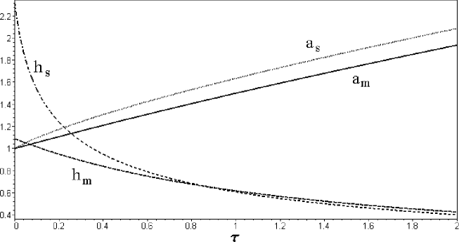
FIG. 1.: Evolution of the scale factors $a_{m}$ and $a_{s}$ for $n=\mu=1$ and $a(0)=1$; $h_{m}$ and $h_{s}$ are the corresponding Hubble coefficients.

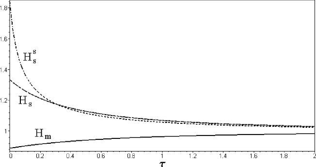
FIG. 2.: Plot of the three quantities $H_{m}$, $H_{s}$ and $H_{s}^{s}$ as defined in the text for the case in Fig. 1.

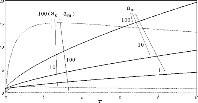
FIG. 3.: Evolution of the scale factors $a_{m}$ and $a_{s}$ for $\mu=1,10,100$.

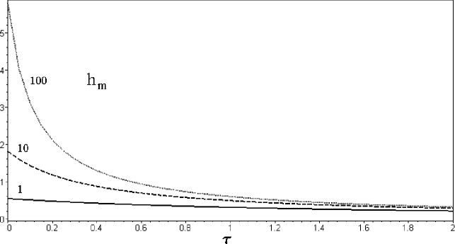
FIG. 4.: Hubble coefficients $h_{m}$ for the trajectories $a_{m}$ in Fig. 3 with $\mu=1,10,100$.

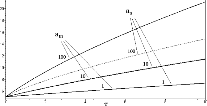
FIG. 5.: Evolution of the scale factors $a_{m}$ and $a_{s}$ for $n=1,10,100$.

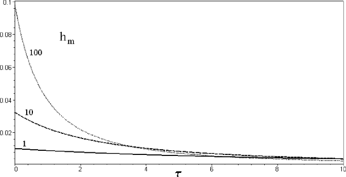
FIG. 6.: Hubble coefficients $h_{m}$ for the trajectories $a_{m}$ in Fig. 5 with $n=1,10,100$.

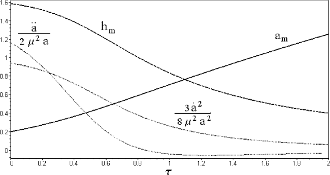
FIG. 7.: Evolution of the scale factor $a_{m}$ for $a_{m}(0)=0.2$, the corresponding Hubble coefficient $h_{m}$ and the ratios between velocity and acceleration of $a_{m}$ and $\mu$.

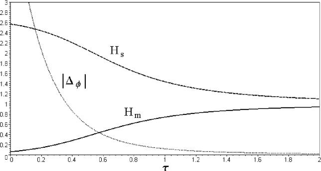
FIG. 8.: Plot of $H_{m}$, $H_{s}$ and $|\Delta_{\phi}|=-\Delta_{\phi}$ for the trajectory in Fig. 7.

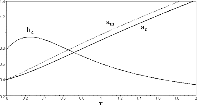
FIG. 9.: Plot of $a_{c}$ and $a_{m}$ with $a(0)=0.4$ and the corresponding Hubble coefficient $h_{c}$.

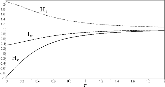
FIG. 10.: Plot of $H_{c}$, $H_{m}$ and $H_{s}$ for the trajectory $a_{c}$ in Fig. 9.

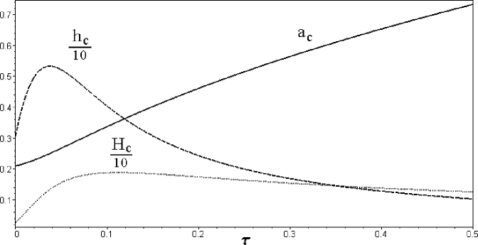
FIG. 11.: Plot of the trajectory $a_{c}$ with $\vec{P}\cdot\vec{P}=n=1$, $k=0$ and $a(0)=0.21$.

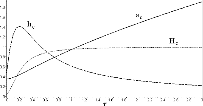
FIG. 12.: Plot of the trajectory $a_{c}$ with $a(0)=0.4$, $h_{c}$ and $H_{c}$.

REFERENCES

- [1] N.D. Birrell and P.C.W. Davies, Quantum fields in curved space, Cambridge University Press, Cambridge, England (1982).
- [2] S.A. Fulling, Gen. Relativ. Gravit. 10, 807 (1979).
- [3] F. Finelli, A. Gruppuso and G. Venturi, Class. Quantum Grav. 16, 3923 (1999).
- [4] E.C.G. Sudarshan and N. Mukunda, Classical dynamics: a modern perspective, R. Klieger Pub. Co., Malabur, Florida (1983).
- [5] H.R. Lewis and W.B. Riesenfeld, J. Math. Phys. 10, 1458 (1969).
- [6] R. Brout and G. Venturi, Phys. Rev. D 39, 2436 (1989). For the general case see [7].
- [7] G. Venturi, “Quantum gravity and the Berry phase”, in Differential geometric methods in theoretical physics, eds. L.-L. Chau and W. Nahm, Plenum, New York (1990).
- [8] C. Bertoni, F. Finelli and G. Venturi, Class. Quantum Grav. 13, 2375 (1996).
- [9] B.S. DeWitt, Phys. Rev. 160, 1113 (1967).
- [10] J.A. Wheeler, in Batelle rencontres: 1967 lectures in mathematics and physics edited by C. DeWitt and J.A. Wheeler, Benjamin, New York (1968).
- [11] C.W. Misner, K.S Thorne and J.A. Wheeler, Gravitation, W.H. Freeman and Co., San Francisco (1973).
- [12] C. Kiefer and T.P. Singh, Phys. Rev. D 44, 1067 (1991).
- [13] R. Casadio and G. Venturi, Class. Quantum Grav. 13, 2715 (1996).
- [14] R. Casadio, F. Finelli and G. Venturi, Class. Quantum Grav. 15, 2451 (1998)
- [15] F. Finelli, G.P. Vacca and G. Venturi, Phys. Rev. D 58, 103514 (1998).
- [16] G.L. Alberghi, R. Casadio, G.P. Vacca and G. Venturi, Class. Quantum Grav. 16, 131 (1999).
- [17] M.S. Madsen, Class. Quantum Grav. 5, 627 (1988).
- [18] B.L. Schumaker, Phys. Rep. 135, 317 (1986).
- [19] B.L. Hu, Stochastic gravity, preprint gr-qc/9902064.
- [20] B.C. DeWitt in Relativity, Groups and Topology, Vol. I, edited by C. DeWitt and B.C. DeWitt, Gordon and Breach, New York (1964).
- [21] P. Hajicek and J. Kijowski, Covariant gauge fixing and Kuchar decomposition, preprint gr-qc/9908051.
- [22] We remark that the full scalar field couples to gravity for . Alternatively one might want to couple only to quantum fluctuations by setting and replacing the factor which multiplies with , but we shall not attempt at this in the present paper.
- [23] In this paper we shall refer to the case with as to the conformally coupled scalar field, although, strictly speaking, such denomination also requires [1].
- [24] One could try to define a new canonical variable such that its conjugate momentum is and diagonalizes the kinetic term in Eq. (40). However, we observe that the explicit form of , as determined by the condition , where is an arbitrary function, would shift the Hamiltonian, , and necessarily mix the gravitational and matter degrees of freedom (for ), to wit . The latter fact places serious questions on the definition of the semiclassical limit for gravity as described in the Introduction, since one cannot disentangle matter from gravity after such a canonical transformation has been performed.
- [25] P. Hajicek, Nucl. Phys. B (Proc. Suppl.) 57, 115 (1997).
- [26] One could avoid most of such formal problems by assuming the (semiclassical) variable is eventually the only physical observable in the system. Since determines the relative positions of freely falling (comoving) points in the Robertson-Walker manifold and space-time points in general relativity are defined only when a material reference frame is introduced [11, 21], this also requires the existence of some (semi)classical matter whose “weight” we shall identify in Eq. (115) with the quantity given in Eq. (108).
- [27] More precisely, there is only one state such that and this gives the classical evolution with .
- [28] V. Frolov, (private communication).
- [29] R. Casadio, On gravitational fluctuations and the semiclassical limit in minisuperspace models, preprint gr-qc/9810073.
- [30] C. Kiefer, Class. Quantum Grav. 4, 1369 (1987).
- [31] X.-C. Gao, J.-B. Xu and T.-Z. Qian, Phys. Rev. A 44, 7016 (1991).
- [32] M. Castagnino, Ann. Inst. Henri Poincaré XXXV, 55 (1981).
- [33] One can also consider a generic superposition of invariant eigenstates , in which case one usually obtains oscillating contributions to (and ) [14, 15].
- [34] V. Faraoni, E. Gunzig and P. Nardone, Conformal transformations in classical gravitational theories and in cosmology, preprint gr-qc/9811047.