Errors on the inverse problem solution for a noisy spherical gravitational wave antenna

Abstract

A single spherical antenna is capable of measuring the direction and polarization of a gravitational wave. It is possible to solve the inverse problem using only linear algebra even in the presence of noise. The simplicity of this solution enables one to explore the error on the solution using standard techniques. In this paper we derive the error on the direction and polarization measurements of a gravitational wave. We show that the solid angle error and the uncertainty on the wave amplitude are direction independent. We also discuss the possibility of determining the polarization amplitudes with isotropic sensitivity for any given gravitational wave source.

1 Introduction

A spherical gravitational wave antenna ideally has equal sensitivity to gravitational waves from all directions and polarizations and is able to determine the directional information and tensorial character of a gravitational wave. The solution for the inverse problem for a noiseless antenna has been known for some time [1], and an analytic solution for an noisy antenna was recently found [2]. These solutions are quite elegant as they only require linear algebra to estimate the wave direction and polarization from the detector outputs.

By monitoring the five quadrupole modes of an elastic sphere, one has a direct measurement of the effective force of a gravitational wave on the sphere [3]. The standard technique for doing so on resonant detectors is to position resonant transducers on the surface of the sphere that strongly couple to the quadrupole modes. A number of proposals have been made for the type and positions of the transducers [4, 5, 6]. What all of these proposals have in common is that the outputs of the transducers are combined into five “mode channels” $g_{m}(t)$ that are constructed to have a one-to-one correspondence with the quadrupole modes of the sphere and thus the spherical amplitudes of the gravitational wave [7, 8].

The mode channels $g_{m}\/$ can be collected to form a “detector response” matrix

$$\bi{A}=\left[\begin{array}[]{ccc}g_{1}-\frac{1}{\sqrt{3}}g_{5}&g_{2}&g_{4}\\ g_{2}&-g_{1}-\frac{1}{\sqrt{3}}g_{5}&g_{3}\\ g_{4}&g_{3}&\frac{2}{\sqrt{3}}g_{5}\end{array}\right],$$ (1)

which, in the absence of noise in the detector, is equal to the GW strain tensor, expressed in lab frame coordinates. The latter tensor has the canonical form

$$\bi{H}=\left[\begin{array}[]{ccc}h_{+}&h_{\times}&0\\ h_{\times}&-h_{+}&0\\ 0&0&0\end{array}\right],$$ (2)

in the wave frame, and is related to $\bi{A}$ by an orthogonal transformation —a rotation. $\bi{H}$ clearly has an eigenvector, $\bi{v}_{3}$, say, with zero eigenvalue which corresponds to the wave propagation direction. The same therefore applies to $\bi{A}$, and this enables the determination of the wave direction by a straightforward algebraic procedure directly from detector data: it is the eigenvector of $\bi{A}$ with null eigenvalue.

Things change when the detector is noisy: noise gets added to the signal in the mode channels, destroying the equivalence between the data matrix $\bi{A}$ and the signal matrix $\bi{H}$. However, it has been shown that under ideal conditions of the noise a modified version of the above procedure can be used [2]: the eigenvector of the noisy $\bi{A}$ with eigenvalue closest to zero is the best approximation to the actual incidence direction of the gravitational wave.

In this paper we shall be taking an analytic approach to the diagonalization problem, whereby errors in the estimated GW parameters can be assessed to any desired degree of accuracy. Inherent in this approach is the unambiguous definition of the incidence direction estimate, as well as a Cartesian coordinate convention for it, which rids us of the ambiguities intrinsically associated to the Euler angle characterization for incidence directions near the Poles. Errors in these quantities will be shown to be incidence direction independent. In addition, we shall also address the problem of estimating the GW amplitudes $h_{+}$ and $h_{\times}$, and their errors. Previous authors [6, 9] found it impossible to give isotropic estimates of these quantities, a very strange result for a spherical detector. We explain why these results come about and we show how the problem can be solved by properly including all the necessary information.

The paper is organized as follows. We begin in section 2 by deriving analytic expressions for the eigenvalues of $\bi{A}$. We then use these expressions to find the first order statistical errors in the eigenvalues in section 3, followed by the direction estimation error in section 4. Higher order corrections to these errors are presented in section 5. In section 6 we discuss the errors on the polarization amplitude estimates. We explain why past solutions have direction dependent errors on these quantities and we describe a maximum likelihood algorithm, based a hypothesis on the physical nature of the source, that fulfills the natural property of source location independence.

2 Detector response eigenvalues

The detector response matrix $\bi{A}$ is symmetric and traceless and has the eigenvalue equation

$$\bi{A}\bi{v}_{k}=\lambda_{k}\bi{v}_{k},\;k=1,2,3,$$ (3)

where the eigenvectors are normalized in the usual way

$$\bi{v}_{k}\cdot\bi{v}_{l}=\delta_{kl}.$$ (4)

Expanding equation (3) we find

$$\lambda_{k}^{3}-g^{2}\lambda_{k}-D=0,$$ (5)

where we have defined

$$g^{2}\equiv g_{1}^{2}+g_{2}^{2}+g_{3}^{2}+g_{4}^{2}+g_{5}^{2}$$ (6a)

$$D\equiv\det(\bi{A}).$$ (6b)

Solving this cubic equation we find the eigenvalues of $\bi{A}$ to be

$$\lambda_{k}=-\frac{2}{\sqrt{3}}\;g\,\cos\theta_{k},\ k=1,2,3,$$ (6g)

where

$$\theta_{k}=\frac{\theta+2(k-1)\pi}{3},\ \mbox{and}\ \cos\theta=-\frac{3\sqrt{3}}{2}\;\frac{D}{g^{3}}.$$ (6h)

The $k=3$ eigenvalue is identically zero in the absence of noise, so it will generally be the one closest to zero in the presence of noise. Random fluctuations may eventually change this (more likely for low SNR), but we shall always take the corresponding eigenvector $\bi{v}_{3}$ as the best approximation to the direction of the source. The amplitude of the wave $h$ can be calculated in many ways from the mode channels (for example, $g\/$ is an estimate for the amplitude), but the semi-difference of the other two eigenvalues will give the best estimate [2],

$$h=\frac{1}{2}\,\left(\lambda_{2}-\lambda_{1}\right).$$ (6i)

3 Eigenvalue errors

We assume that the mode channels $g_{m}$ have uncorrelated noise with zero mean and variance $\sigma_{g_{m}}^{2}\equiv E\left\{(\delta g_{m})^{2}\right\}$. The lowest order statistical errors in the eigenvalues are easily calculated by

$$\sigma_{\lambda_{k}}^{2}=\sum_{m=1}^{5}\left(\frac{\partial\lambda_{k}}{\partial g_{m}}\right)^{2}\sigma_{g_{m}}^{2},$$ (6j)

where the derivatives of the eigenvalues are given by

$$\frac{\partial\lambda_{k}}{\partial g_{m}}=-\frac{2}{\sqrt{3}}\;\frac{g_{m}}{g}\,\cos\theta_{k}+\frac{\partial D}{\partial g_{m}}\,\sin\theta_{k},$$ (6k)

and the derivatives of the determinant $D\/$ are

$$\frac{\partial D}{\partial g_{1}} = -\frac{4}{\sqrt{3}}g_{1}g_{5}-g_{3}^{2}+g_{4}^{2},$$ (6la)

$$\frac{\partial D}{\partial g_{2}} = -\frac{4}{\sqrt{3}}g_{2}g_{5}+2g_{3}g_{4},$$ (6lb)

$$\frac{\partial D}{\partial g_{3}} = -2g_{3}\left(g_{1}-\frac{g_{5}}{\sqrt{3}}\right)+2g_{2}g_{4},$$ (6lc)

$$\frac{\partial D}{\partial g_{4}} = 2g_{4}\left(g_{1}+\frac{g_{5}}{\sqrt{3}}\right)+2g_{2}g_{3},$$ (6ld)

$$\frac{\partial D}{\partial g_{5}} = \frac{1}{\sqrt{3}}\,\left(-2g_{1}^{2}-2g_{2}^{2}+g_{3}^{2}+g_{4}^{2}+2g_{5}^{2}\right).$$ (6le)

If the variances on the mode channels are equal then it is easily seen that equations (6j) and (6k) lead to

$$\sigma_{\lambda_{k}}^{2}=\frac{4}{3}\,\sigma_{g}^{2},\ k=1,2,3,$$ (6lm)

where $\sigma_{g}^{2}$ is the variance on any one mode channel. Note that from equation (6lm) all three eigenvalues have equal variance to first order. Cross correlations between these eigenvalues are also easily calculated, and for equal mode channel variances they are equal for all pairs $(\lambda_{k},\lambda_{k}^{\prime})$:

$$\sigma_{\lambda_{k}\lambda_{k}^{\prime}}=-\frac{2}{3}\,\sigma_{g}^{2},\ k,k^{\prime}=1,2,3.$$ (6ln)

Shown in Figs. 1-3 is this variance as a function of the ${\rm SNR}=g^{2}/\sigma_{g}^{2}$. Also shown is the results of a Monte Carlo type simulation of the errors which take into account the higher order perturbations at low values of SNR. As shown, the analytic expressions match the simulated errors for high SNR. For low SNR discrepancies arise between the analytic and simulated values. This is within expectation since equation (6lm) is only accurate for large SNR. Higher order correction will be considered below.

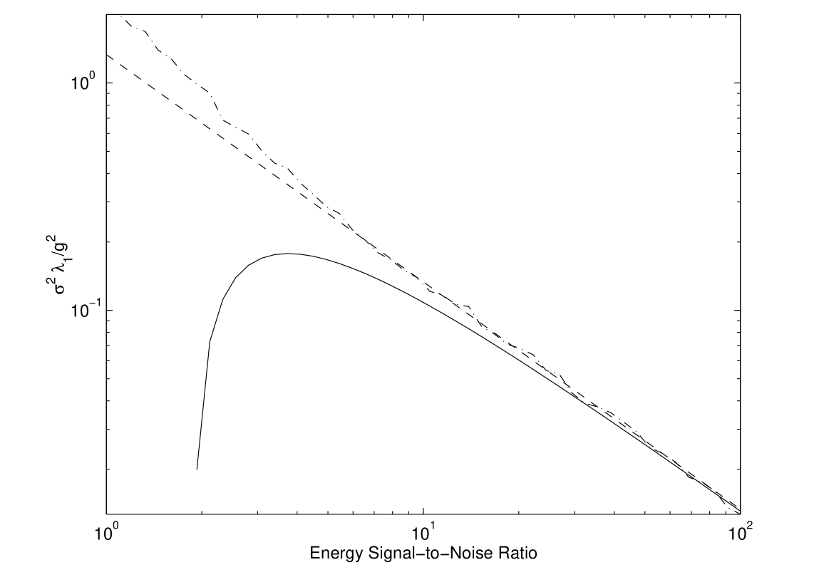
Figure 1: The results of a numerical simulation describing the variance of the first eigenvalue for a range of SNR. The dot-dashed line was computed by a 1000 trial Monte Carlo simulation for the range of SNR. The dashed line is the error found from the first order analytic expression and the solid line includes the second order corrections.

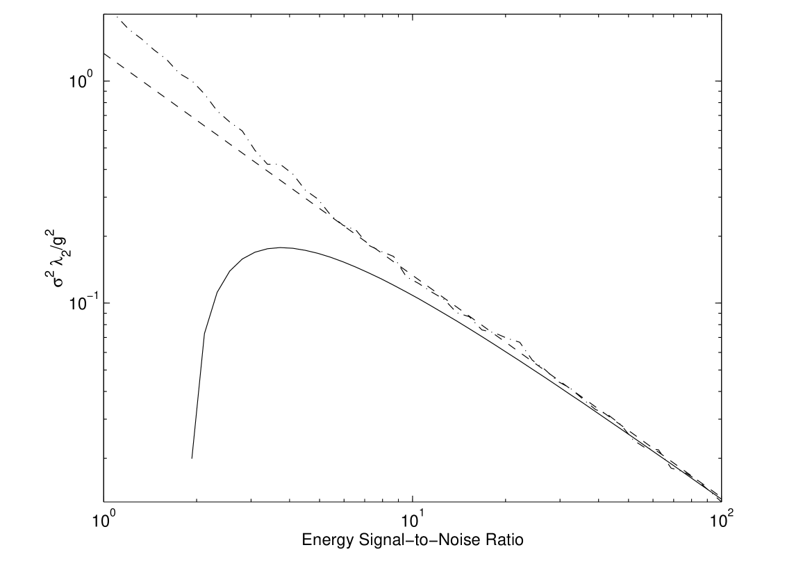
Figure 2: The results of a numerical simulation describing the variance of the second eigenvalue for a range of SNR. The dot-dashed line was computed by a 1000 trial Monte Carlo simulation for the range of SNR. The dashed line is the error found from the first order analytic expression and the solid line includes the second order corrections.

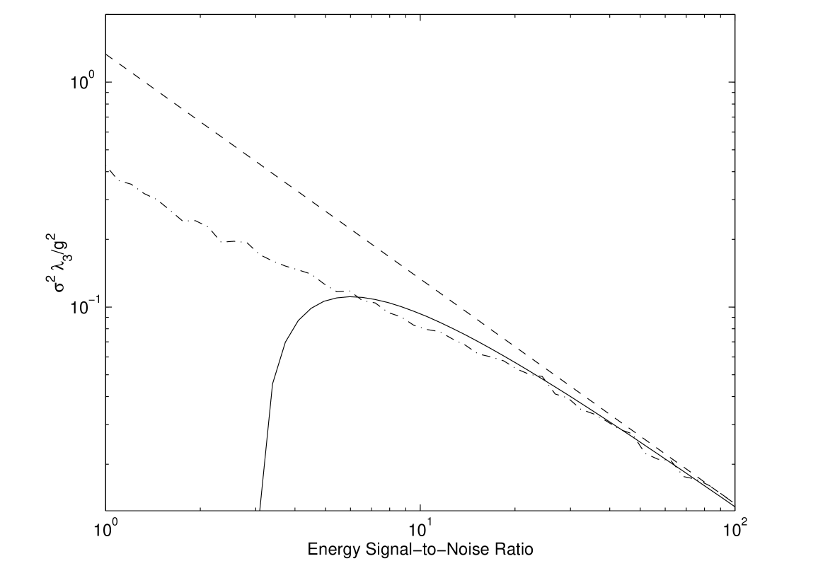
Figure 3: The results of a numerical simulation describing the variance of the third eigenvalue for a range of SNR. The dot-dashed line was computed by a 1000 trial Monte Carlo simulation for the range of SNR. The dashed line is the error found from the first order analytic expression and the solid line includes the second order corrections.

4 Direction estimation error

We assume that the eigenvector $\bi{v}_{3}$ points in the propagation direction of the gravitational wave. We want to estimate the fluctuations in the determination of this direction caused by the presence of noisy fluctuations in the mode channels. We represent with $\delta$ a difference between a given quantity and its ideal value if there were no noise (i.e. $\delta\bi{v}_{3}$ is the difference between the position calculated from noisy data and its real position in the sky). We now take equation (3) for $k=3$ and consider fluctuations in it. If these are not too large (high SNR) we can retain only first order terms

$$\left[\bi{A}-\lambda_{3}\right]\delta\bi{v}_{3}=-\left[\delta\bi{A}-\delta\lambda_{3}\right]\bi{v}_{3}.$$ (6lo)

This is an equation for $\delta\bi{v}_{3}$, but the matrix $\left[\bi{A}-\lambda_{3}\right]$ is not invertible. The only consequence of this is that we cannot determine the component of $\delta\bi{v}_{3}$ which is parallel to $\bi{v}_{3}$ itself. The orthogonal components (those parallel to $\bi{v}_{1}$ and $\bi{v}_{2}$) can easily be found by multiplying equation 6lo on the left by $\bi{v}_{1}$ and $\bi{v}_{2}$

$$\bi{v}_{1}\cdot\delta\bi{v}_{3} = -\frac{1}{\lambda_{1}-\lambda_{3}}\;\bi{v}_{1}\delta\bi{A}\bi{v}_{3},$$ (6lp)

$$\bi{v}_{2}\cdot\delta\bi{v}_{3} = -\frac{1}{\lambda_{2}-\lambda_{3}}\;\bi{v}_{2}\delta\bi{A}\bi{v}_{3}.$$ (6lq)

An appropriate assessment of the error on a direction measurement is the solid angle error $\Delta\Omega$. Since $|\bi{v}_{3}|=1$, this error is given by

$$\Delta\Omega=\pi\left|\Delta\bi{v}_{3}\right|^{2}.$$ (6lr)

where $|\Delta\bi{v}_{3}|^{2}$ is the quadratic error in the determination of $\bi{v}_{3}$. To find it we need to calculate the expectation of the squared modulus of the above fluctuations,

$$\left|\Delta\bi{v}_{3}\right|^{2}=E\left\{(\bi{v}_{1}\cdot\delta\bi{v}_{3})^{2}+(\bi{v}_{2}\cdot\delta\bi{v}_{3})^{2}\right\}=E\left\{\left|\frac{\bi{v}_{1}\delta\bi{A}\bi{v}_{3}}{\lambda_{1}-\lambda_{3}}\right|^{2}+\left|\frac{\bi{v}_{2}\delta\bi{A}\bi{v}_{3}}{\lambda_{2}-\lambda_{3}}\right|^{2}\right\}.$$ (6ls)

First order calculations only require us to take expectations in $\delta\bi{A}$, while leaving the rest untouched,

$$\delta\bi{A}=\sum_{m=1}^{5}\bi{A}_{m}\delta g_{m},$$ (6lt)

where we have defined

$$\bi{A}_{m}\equiv\frac{\partial\bi{A}}{\partial g_{m}},$$ (6lu)

Explicitly,

$$\qquad\ \ \ \ \bi{A}_{1}=\left[\begin{array}[]{ccc}1&0&0\\ 0&-1&0\\ 0&0&0\end{array}\right],\ \bi{A}_{2}=\left[\begin{array}[]{ccc}0&1&0\\ 1&0&0\\ 0&0&0\end{array}\right],\ \bi{A}_{3}=\left[\begin{array}[]{ccc}0&0&0\\ 0&0&1\\ 0&1&0\end{array}\right],$$ (6lvj)

$$\bi{A}_{4}=\left[\begin{array}[]{ccc}0&0&1\\ 0&0&0\\ 1&0&0\end{array}\right],\ \bi{A}_{5}=\left[\begin{array}[]{ccc}-\frac{1}{\sqrt{3}}&0&0\\ 0&-\frac{1}{\sqrt{3}}&0\\ 0&0&\frac{2}{\sqrt{3}}\end{array}\right].$$ (6lvq)

We thus have

$$|\Delta\bi{v}_{3}|^{2}=\sum_{m=1}^{5}\left[\left(\bi{v}_{1}\bi{A}_{m}\bi{v}_{3}\right)^{2}+\left(\bi{v}_{2}\bi{A}_{m}\bi{v}_{3}\right)^{2}\right]\,\frac{\sigma_{g_{m}}^{2}}{g^{2}}.$$ (6lvw)

Again, setting the variances on the mode channels equal to $\sigma_{g}^{2}$, the sum in equation (6lvw) can easily be done, giving

$$|\Delta\bi{v}_{3}|^{2}=2\,\frac{\sigma_{g}^{2}}{g^{2}}.$$ (6lvx)

From equation (6lvx) we see that the error in the incidence direction is independent of this direction, as expected of an omnidirectional antenna. Substituting this into (6lr) we find

$$\Delta\Omega=\frac{2\pi}{SNR}.$$ (6lvy)

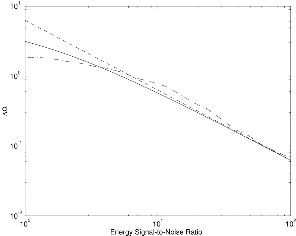
Figure 4: The results of a numerical simulation describing the solid angle direction estimation error $\Delta\Omega$ of a source direction measurement due to a finite signal-to-noise ratio. The dot-dashed line was computed by a 1000 trial Monte Carlo simulation for the range of SNR. The dashed line is the error found from the first order analytic expression and the solid line includes the second order corrections.

This expression is in perfect agreement with the solid angle estimation error found by Zhou and Michelson who used a maximum likelihood technique to estimate the wave direction [6]. This is not surprising as the two methods of estimating the wave direction have been shown to be equivalent (though the assumptions behind each are quite different) [2]. The advantage of our approach is that, by using unit vectors (Cartesian components), we are all the time free from the anomalously high errors and correlations intrinsically associated to the Euler angle parametrization.

Shown in Fig. 4 is the solid angle estimation error as a function of the SNR. Also shown is the results of a Monte Carlo type simulation of the errors. As shown, the analytic expressions match the simulated errors for high SNR. Deviations however appear for lower values of SNR. This again is due to the insufficiency of the first order analytical estimates of the errors. In the next section we present improved theoretical estimates of the errors by going one order beyond the first in the calculations of variances.

5 Higher order corrections

In order to improve our theoretical understanding of the error behaviours of the Monte Carlo simulations displayed in Figs. 1-4 we need to go one step beyond the linear error terms of equations (6j) and (6lvw). This requires calculations of higher order derivatives for the added terms, and then the resulting general expressions become quite complicated. They somewhat simplify for equal mode channel variances, but are still rather cumbersome. For example, the next order correction to the eigenvalues, assuming the mode channel noises are zero-mean independent Gaussian processes, is given by (see appendix)

$$\sigma_{\lambda_{k}}^{2}=\frac{4}{3}\,\sigma_{g}^{2}+$$

$$+\left(\sum_{m,m^{\prime}=1}^{5}\,\frac{\partial\lambda_{k}}{\partial g_{m}}\;\frac{\partial^{3}\lambda_{k}}{\partial g_{m}\,\partial g_{m^{\prime}}\,\partial g_{m^{\prime}}}+\frac{1}{2}\,\frac{\partial^{2}\lambda_{k}}{\partial g_{m}\,\partial g_{m^{\prime}}}\,\frac{\partial^{2}\lambda_{k}}{\partial g_{m}\,\partial g_{m^{\prime}}}\right)\;\sigma_{g}^{4},\ \ \ k=1,2,3,$$ (6lvz)

After rather long algebra it is found that

$$\sigma_{\lambda_{k}}^{2}=\frac{4}{3}\,\sigma_{g}^{2}-2\,\left(1+\sin^{2}\theta_{k}\right)\;\frac{\sigma_{g}^{4}}{g^{2}}.$$ (6lvaa)

It turns out that the series for $\sigma_{\lambda_{k}}^{2}$ converges very slowly for low SNR, so that equation (6lvz) only constitutes an improvement on (6j) for a rather limited range of SNR —see Figs. 1-3. Equation (6lvaa) shows that the errors in $\lambda_{1}$ and $\lambda_{2}$ split from the error in $\lambda_{3}$ for low values of SNR, and reproduces the observed behaviour that $\sigma_{\lambda_{3}}^{2}$ falls below $\sigma_{\lambda_{1}}^{2}$ and $\sigma_{\lambda_{2}}^{2}$. It is a reasonable approximation to $\sigma_{\lambda_{3}}^{2}$ for SNR between 30 and 6, but it is not quite as good as regards $\sigma_{\lambda_{1}}^{2}$ and $\sigma_{\lambda_{2}}^{2}$ for those values of SNR. Higher order terms would be required for an improvement, but these imply still much longer calculations of derivatives of the eigenvalues up to the fifth order, as can be seen in equation (6lvadaeafap) of the appendix.

Similar corrections can be applied to the incidence direction error estimate of equation (6lvx). They appear to be given by

$$|\Delta\bi{v}_{3}|^{2}=2\,\frac{\sigma_{g}^{2}}{g^{2}}\,\left(1+\frac{\sigma_{g}^{2}}{g^{2}}\right)^{-1}$$ (6lvab)

for equal mode channel variances, $\sigma_{g}^{2}$. Solid angle errors can be directly inferred from here:

$$\Delta\Omega=\frac{2\pi}{SNR}\;\left(1+SNR^{-1}\right)^{-1}.$$ (6lvac)

As shown in Fig. 4, the above theoretical prediction is a better approach to the behaviour observed in the numerical simulations than is equation (6lvy). For SNR less than 2, equation (6lvac) is also insufficient.

It is important to remind ourselves that for very low SNR the uncertainties on the direction estimation are so large that the measurement is almost meaningless. Zhou and Michelson decided that a minimum SNR of 10 in energy was necessary for a direction measurement [6]. Looking at Fig. 4 this lower limit seems reasonable, thus it is only necessary to have accurate analytical expressions down to that level.

6 Polarization amplitudes

We now come to the discussion of errors in the polarization amplitudes $h_{+}$ and $h_{\times}$. It is easily shown that the uncertainty on the measurement of the polarization amplitudes is direction independent if the source position is known ahead of time [6], but it has been claimed that in the unknown direction case there is a strong direction dependency [9]. This is disturbing given that a spherical detector is equally sensitive to waves of all polarization and direction. We argue in this section that the difficulties to find isotropic estimates of $h_{+}$ and $h_{\times}$ are ultimately due to the use of unsuitable criteria to set up those estimates. We discuss a more natural procedure, based on data set processing, that leads to a solution of this problem.

To understand why a simple estimate of the errors leads to direction dependencies, let us look at the basics of the solution to the inverse problem. We are given 3 eigenvectors and 3 eigenvalues, but these are not independent. The eigenvectors are orthogonal, so we actually only get 2 pieces of information from them. We use that information to determine the direction of the wave. Next, the strain tensor is traceless so the third eigenvalue can be determined from the other two, therefore, we only get 2 pieces of information from them. We use one of them (actually a combination of 2) to get the wave amplitude. Past reasoning suggested that we can use the last piece of information to determine the polarization angle. This is wrong. The last eigenvalue does not tell us the polarization, but rather is related to the scalar component of the GW (or lack thereof). We assume this to be zero for GR, so this can be interpreted as a measurement of the non-zeroness of this component. The fact that we decide that this should be zero a priori does not give us additional information about the polarization, only the level of noise in our system. Without any additional information we have an under-determined system which will lead to direction dependent errors as seen in reference [9].

The additional piece of information needed is the polarization angle $\alpha$: the angle between the GW’s axes and the eigenvectors $\bi{v}_{1}$ and $\bi{v}_{2}$ perpendicular to the incidence direction $\bi{v}_{3}$. To this end, we submit our diagonal form of the matrix $\bi{A}$ to a rotation of angle $\alpha$ about $\bi{v}_{3}$ to obtain best estimates of $h_{+}$ and $h_{\times}$ by the formulas

$$h_{+} = h\cos 2\alpha,$$ (6lvada)

$$h_{\times} = h\sin 2\alpha,$$ (6lvadb)

where the pure and uncorrelated noise term in $h_{+}$ was dropped out. The GW amplitude $h\/$ $\equiv$ $(h_{+}^{2}+h_{\times}^{2})^{1/2}$ has been shown to have a best estimate given by equation (6i). $h\/$ can be determined with isotropic sensitivity since that is the case with $\lambda_{1}$ and $\lambda_{2}$, as we have just seen. For a fixed $\alpha$, equations (6lvada) and (6lvadb) give us an estimate of $h_{+}$ and $h_{\times}$ in the presence of noise in the detector.

We can use the results of section 3 to see that

$$\sigma_{+}^{2} = \cos^{2}2\alpha\,\sigma_{g}^{2}$$ (6lvadaea)

$$\sigma_{\times}^{2} = \sin^{2}2\alpha\,\sigma_{g}^{2}$$ (6lvadaeb)

$$\sigma_{+\times} = -\frac{1}{2}\,\sin 4\alpha\,\sigma_{g}^{2}$$ (6lvadaec)

and these errors are indeed isotropic, for they only depend on $\sigma_{g}$.

In the absence of further information on the specific physical nature of the source, any polarization angle $\alpha\/$ is valid, for the canonical form of the tensor (2) is invariant to rotations about the third axis. A particular choice of $\alpha\/$ is thus a matter of taste in this case, and equations (6lvadaea)–(6lvadaec) give the correct error estimates. A common way [1] to resolve the arbitrariness in $\alpha\/$ is to set the first Euler angle in the rotation relating the lab frame to the wave frame equal to zero.

However, this is a very much observer dependent criterion, for detectors at different locations would claim different values for $h_{+}$ and $h_{\times}$, even if they agreed to be seeing the same source. Errors in $h_{+}$ and $h_{\times}$ based on such criterion have been shown e.g. by [9] to be strongly direction dependent, which is certainly not surprising. It is however paradoxical that a spherical detector should prefer certain directions to others to detect a GW signal, therefore this must be reassessed. We now propose a more consistent solution.

It is clear from the above discussion that any criterion to resolve the arbitrariness in $\alpha\/$, therefore to estimate $h_{+}$ and $h_{\times}$, should be established relatively to the GW source, be it known ahead of time or based on a hypothesis to be checked a posteriori.

Let us, for concreteness, consider a coalescing binary system as the GW source [10]. The signal generated by such a system is given by somewhat complicated functions of the space-time variables and a number of system parameters; it will not be necessary for our purposes to consider in detail the explicit form of such functions (see for example [11]), it will suffice to use formal expressions indicating the signal dependencies:

$$h_{+} = h_{+}(\bi{r},t;{\cal K}),$$ (6lvadaeafa)

$$h_{\times} = h_{\times}(\bi{r},t;{\cal K}).$$ (6lvadaeafb)

Here $\bi{r}\/$ is the source position, and $t\/$ is the time. ${\cal K\/}$ stands for the set of characteristic source parameters, which in this case include the masses of the stars, the inclination of the orbital plane, the semimajor axis, the eccentricity of the orbit, the periastron position, etc. Note that these amplitudes are referred to a set of source axes, so they are independent of the detector’s location.

The usual way to estimate the parameters ${\cal K\/}$ is to resort to classical Statistics [12], as has been done for example in [13] for interferometric detectors or in [9] for spherical detectors. The fundamental quantity required by such method is the likelihood function, $\Lambda$, which is a functional of the (unknown) signal parameters and the detector data.

We then proceed as follows: we construct the likelihood function associated to the hypothesis that equations (6lvada) and (6lvadb) be a fit to equations (6lvadaeafb) and (6lvadaeafb) for suitable values of the parameters $\cal K\/$. It will thus have the generic form

$$\Lambda=\Lambda(h;\alpha;{\cal K})$$ (6lvadaeafag)

Standard manipulations of $\Lambda$ yield both best estimates of the signal parameters ${\cal K\/}$ and of the polarization angle $\alpha\/$, as well as errors and cross correlations between any pair of these —it is recalled that such are identified as the coefficients of the covariance matrix, which is the inverse of the matrix of second derivatives of $\Lambda$ [12].

We shall not attempt to give a detailed discussion of this process here. The important point to stress is that in the approach just proposed, we have managed to have $h\/$ as the only combination of actual data entering the likelihood function $\Lambda$. Errors and cross correlations between parameter estimates will thus ultimately be functions only of the errors and cross correlations between the eigenvalue estimates, $\lambda_{1}$ and $\lambda_{2}$, which we have proved in section 3 to be direction independent.

So not only $\alpha\/$ but also the source parameters ${\cal K\/}$ can be determined with isotropic sensitivity by means of a spherical GW detector. The same therefore applies to the GW amplitudes $h_{+}$ and $h_{\times}$, as indeed expected.

The quantitative estimation of the errors in $h_{+}$ and $h_{\times}$ cannot however be given explicitly until the full parameter estimation problem has been completely solved, as interactions between all those estimates will strongly affect one another.

7 Discussion

With analytic expressions for the uncertainties on the eigenvectors and the eigenvalues of the mode channel matrix (1) we can turn our attention to the physical interpretation of these values. An unambiguous selection of $\lambda_{3}$ can be made on the basis that it is the third root in equation (6g). This will usually be the one closest to zero. Then the other two represent the amplitude measurement. As proved in [2], the best estimate of the GW amplitude is the semi-difference of these two, $(\lambda_{2}-\lambda_{1})/2$.

The third eigenvalue ideally should be zero if general relativity is correct. Once noise is introduced this is no longer the case, but the variance on this eigenvalue gives us a level of the “non-zeroness”. One can imagine setting a threshold on this eigenvalue that is a function of $\sigma_{\lambda_{3}}$ (a function of the SNR) to veto any candidate events that have an excessive $\lambda_{3}$. Many non-GW sources are likely to produce a non-zero $\lambda_{3}$, therefore becoming easily identified and discarded.

The errors in both eigenvalues and eigenvectors are direction independent. The last step in the analysis is the splitting of the GW amplitude $h\/$ into the usual $h_{+}$ and $h_{\times}$ components. We have shown that this can be accomplished by making suitable reference to the source properties, whereby isotropic sensitivity to these quantities obtains. This solves the paradox of the anisotropies in the determination of $h_{+}$ and $h_{\times}$, and stresses the fact that the most fundamental magnitudes to estimate from the detector data are the eigenvalues and eigenvectors of the mode channel matrix: these are source independent, and any further progress in signal deconvolution explicitly requires reference to the source properties, be them known ahead of time or be them stated in the form of a hypothesis to test.

Appendix A Quadratic error calculations

Let $\bi{g}=(g_{1},\,\ldots\,,g_{n})$ be a set of $n\/$ independent Gaussian random variables, with mean $\bi{\mu}=(\mu_{1},\,\ldots\,,\mu_{n})$ and variances $\sigma_{i}^{2}\ (i=1,...,n)$. Let $f(\bi{g})$ be a regular function of its arguments. Because $\bi{g}$ is a random variable so is $f(\bi{g})$, although it will of course be generally non-Gaussian. We want to find the mean and variance of $f(\bi{g})$, and to this end we Taylor expand it around the mean $\bi{\mu}\/$:

$$f(\bi{g})=f(\bi{\mu})+f_{i}\,\delta g_{i}+\frac{1}{2}\,f_{ij}\,\delta g_{i}\,\delta g_{j}+\frac{1}{6}\,f_{ijk}\,\delta g_{i}\,\delta g_{j}\,\delta g_{k}+\ldots$$ (6lvadaeafah)

where

$$f_{ij\ldots}\equiv\left.\frac{\partial f}{\partial g_{i}\partial g_{j}\ldots}\right|_{\bi{g}=\bi{\mu}}\ \ \ \mbox{and}\ \ \ \delta g_{i}\equiv g_{i}-\mu_{i}.$$ (6lvadaeafai)

and the usual convention of summation over repeated indices is adopted in (6lvadaeafah).

The mean of $f(\bi{g})$ is its expectation value, $E\{f(\bi{g})\}$, while its variance is the difference

$$\sigma_{f}^{2}=E\{f^{2}(\bi{g})\}-[E\{f(\bi{g})\}]^{2}$$ (6lvadaeafaj)

Expectation values are to be taken on the basis of the expansion (6lvadaeafah). Given that $\bi{g}$ is a set of independent Gaussian variables, the expectation of the product of an odd number of $\delta g$’s is zero, while

$$E\{\delta g_{i}\,\delta g_{j}\} = \delta_{ij}\,\sigma_{i}^{2}$$ (6lvadaeafak)

$$E\{\delta g_{i}\,\delta g_{j}\,\delta g_{k}\,\delta g_{l}\} = \delta_{ij}\,\delta_{kl}\;\sigma_{i}^{2}\,\sigma_{k}^{2}+\delta_{ik}\,\delta_{jl}\;\sigma_{i}^{2}\,\sigma_{j}^{2}+\delta_{il}\,\delta_{jk}\;\sigma_{i}^{2}\,\sigma_{j}^{2}$$ (6lvadaeafal)

etc., where no summation over repeated indices is exceptionally assumed in these expressions. If the assumption is made that all the $g\/$’s have equal variances, $\sigma^{2}$, then one easily finds

$$E\{f(\bi{g})\}=f+\frac{1}{2}\,f_{ii}\;\sigma^{2}+\frac{1}{8}\,f_{iijj}\;\sigma^{4}+\frac{1}{48}\,f_{iijjkk}\;\sigma^{6}+\ldots$$ (6lvadaeafam)

where $f\/$ is a shorthand for $f(\bi{\mu})$. Likewise,

$$\left[E\{f(\bi{g})\}\right]^{2}=f^{2}+ff_{ii}\;\sigma^{2}+\frac{1}{4}\,\left(ff_{iijj}+f_{ij}f_{ij}\right)\,\sigma^{4}$$

$$+\frac{1}{24}\,\left(ff_{iijjkk}+3\,f_{ij}f_{ijkk}\right)\,\sigma^{6}+\ldots,$$ (6lvadaeafan)

and

$$E\{f^{2}(\bi{g})\}=f^{2}+\left(ff_{ii}+f_{i}f_{i}\right)\,\sigma^{2}+\frac{1}{4}\,\left(ff_{iijj}+4\,f_{i}f_{ijj}+3\,f_{ij}f_{ij}\right)\,\sigma^{4}$$

$$+\frac{1}{24}\,\left(ff_{iijjkk}+6\,f_{i}f_{ijjkk}+15\,f_{ij}f_{ijkk}+10\,f_{ijk}f_{ijk}\right)\,\sigma^{6}+\ldots$$ (6lvadaeafao)

So, finally,

$$\sigma_{f}^{2}=f_{i}f_{i}\;\sigma^{2}+\left(f_{i}f_{ijj}+\frac{1}{2}\,f_{ij}f_{ij}\right)\,\sigma^{4}bb$$

$$\hbox to0.0pt{\hss${}+{}$}\frac{1}{4}\,\left(f_{i}f_{ijjkk}+2\,f_{ij}f_{ijkk}+\frac{5}{3}\,f_{ijk}f_{ijk}\right)\,\sigma^{6}+\ldots$$ (6lvadaeafap)

References

References

- [1] Wagoner R V and Paik H J 1976 Proceedings of International Symposium on Experimental Gravitation, Pavia (Roma Accademia Nazionale dei Lincei, Roma) p 257
- [2] Merkowitz S M 1998 Phys Rev D 58 062002
- [3] Lobo J A Phys. Rev. D 1995 52 591
- [4] Johnson W W and Merkowitz S M 1993 Phys Rev Lett 70 2367
- [5] Lobo J A and Serrano M A 1996 Europhys Lett 35 253
- [6] Zhou C and Michelson P F 1995 Phys Rev D 51 2517
- [7] Merkowitz S M and Johnson W W 1995 Phys Rev D 51 2546
- [8] Lobo J A 1997 in Mathematics of Gravitation edited by A. Królak, Banach Center Publications, volume 41, Warsaw (Poland)
- [9] Stevenson T R 1997 Phys Rev D 56 564
- [10] Coccia E and Fafone V 1996 Phys Lett A 213 16
- [11] Moreno-Garrido C, Buitrago J and Mediavilla E 1994 Monthly Notices of the Royal Astronomical Society 266 16, and 1995 274 115
- [12] Helstrom C W 1968 Statistical Theory of Signal Detection (Oxford: Pergamon Press)
- [13] Królak A, Lobo J A and Meers B J 1993 Phys Rev D 48 3451