Numerical Relativity As A Tool For Computational Astrophysics

Abstract

The astrophysics of compact objects, which requires Einstein’s theory of general relativity for understanding phenomena such as black holes and neutron stars, is attracting increasing attention. In general relativity, gravity is governed by an extremely complex set of coupled, nonlinear, hyperbolic-elliptic partial differential equations. The largest parallel supercomputers are finally approaching the speed and memory required to solve the complete set of Einstein’s equations for the first time since they were written over 80 years ago, allowing one to attempt full 3D simulations of such exciting events as colliding black holes and neutron stars. In this paper we review the computational effort in this direction, and discuss a new 3D multi-purpose parallel code called “Cactus” for general relativistic astrophysics. Directions for further work are indicated where appropriate.

1 Overview

The Einstein equations for the structure of spacetime were first published in 1916 when Einstein introduced his famous general theory of relativity. This theory of gravity has remained essentially unchanged since its discovery, and it provides the underpinnings of modern theories of astrophysics and cosmology. The theory is essential in describing phenomena such as black holes, compact objects, supernovae, and the formation of structure in the Universe. Unfortunately, the equations are a set of highly complex, coupled, nonlinear partial differential equations involving 10 functions of 4 independent variables. They are among the most complicated equations in mathematical physics. For this reason, in spite of more than 80 years of intense study, the solution space to the full set of equations is essentially unknown. Most of what we know about this fundamental theory of physics has been gleaned from linearized solutions, highly idealized solutions possessing a high degree of symmetry (e.g., static, or spherically or axially symmetric), or from perturbations of these solutions.

Over the last 30 years a growing research area, called Numerical Relativity, has developed, where computers are employed to construct numerical solutions to these equations. Although much has been learned through this approach, progress has been slow due to the complexity of the equations and inadequate computational power. For example, an important astrophysical application is the 3D spiraling coalescence of two black holes (BH) or neutron stars (NS), which will generate strong sources of gravitational waves. As has been emphasized by Flanagan and Hughes, one of the best candidates for early detection by the laser interferometer network is increasingly considered to be BH mergers[1, 2]. The imminent arrival of data from the long awaited gravitational wave interferometers (see, e.g., Ref. [1] and references therein) has provided a sense of urgency in understanding these strong sources of gravitational waves. Such understanding can be obtained only through large scale computer simulations using the full machinery of numerical relativity.

Furthermore, the gravitational wave signals are likely to be so weak by the time they reach the detectors that reliable detection may be difficult without prior knowledge of the merger waveform. These signals can be properly interpreted, or perhaps even detected, only with a detailed comparison between the observational data and a set of theoretically determined “waveform templates”. In most cases, these waveform templates needed for gravitational wave data analysis have to be generated by large scale computer simulations, adding to the urgency of developing numerical relativity. However, a realistic 3D simulation based on the full Einstein equations is a highly non-trivial task—based on axisymmetric black hole calculations performed during late 1980’s and algorithms available at the time—one can estimate the time required for a reasonably accurate 3D simulation of, say, the coalescence of a compact object binary, to be at least 100,000 Cray Y-MP hours!

But there is good reason for optimism that such problems can be solved within the next decade. Scalable parallel computers, and efficient algorithms that exploit them, are quickly revolutionizing computational science, and numerical relativity is a great beneficiary of these developments. Over the last years the community has developed 3D codes designed to solve the complete set of Einstein equations that run very efficiently on large scale parallel computers. We will describe below one such code, called “Cactus”, that has achieved 142 GFlops on a 1024 node Cray T3E-1200, which is more than 2000 times faster than 2D codes of a few years ago running on a Cray Y-MP (which also had only about 0.5% the memory capacity of the large T3E). Such machines are expected to scale up rapidly as faster processors are connected together in even higher numbers, achieving Teraflop performance on real applications in a few years.

Numerical relativity requires not only large computers and efficient codes, but also a wide variety of numerical algorithms for evolving and analyzing the solution. Because of this richness and complexity of the equations, and the interesting applications to problems such as black holes and neutron stars, natural collaborations have developed between applied mathematicians, physicists, astrophysicists, and computational scientists in the development of a single code to attack these problems. There are various large scale collaborative effort in recent years in this direction, including the NSF Black Hole Grand Challenge Project (recently concluded), the NASA Neutron Star Grand Challenge Project and the NCSA/Potsdam/Wash U numerical relativity collaboration.

We introduce in this paper a code called “Cactus”, which is developed by the NCSA/Potsdam/Wash U collaboration, and is employed in the NASA Neutron Star Grand Challenge Project. We will describe some of the algorithms and capabilities of this code in this paper. In the next sections we will first give a brief description of the numerical formulation of the theory of general relativity, and discuss particular difficulties associated with numerical relativity. The discussion will necessarily be brief. Examples are mostly drawn from work carried out by our NCSA/Potsdam/Wash U numerical relativity collaboration. We also provide URL addresses for web pages containing graphics and movies of some of our results.

To conclude this brief introduction, a statement of where we stand in terms of simulating general relativistic compact objects is in order. The NSF black hole grand challenge project and related work achieved long term stable evolution of single black hole spacetimes under certain conditions [3, 4, 5], but there is still a long way to go before the spiraling coalescence can be computed. The presently on-going NASA neutron star grand challenge project recently succeeded in evolving grazing collision of two neutron stars using the full Einstein-relativistic hydrodynamic system of equations, with a simple equation of state. While the inspiral coalescences of two neutron stars is not a stated goal of the NASA project, we expect to be able to carry out preliminary studies of the inspiral coalescences in the next few years. The final goal of a full solution of the problem including radiation transport and magneto-hydrodynamics for comparison between numerical simulations and observations in gravitational wave astronomy (waveform templates) and high energy astronomy ($gamma$ ray burst) will take many more years, hopefully building on the effort described in this paper. The Nakamura group also reports preliminary success in evolving several orbits with a fully relativistic GR-hydro code [6].

2 Einstein Equations for Relativity

The generality and complexity of the Einstein equations make them an excellent and fertile testing ground for a variety of broadly significant computing issues. They form a system of dozens of coupled, nonlinear equations, with thousands of terms, of mixed hyperbolic-elliptic type, and even undefined types, depending on coordinate conditions. This rich and general structure of the equations implies that the techniques developed to solve our problems will be immediately applicable to a large family of diverse scientific applications.

The system of equations breaks up naturally into a set of constraint equations, which are elliptic in nature, evolution equations, which are “hyperbolic” in nature (more on this below), and gauge equations, which can be chosen arbitrarily (often leading to more elliptic equations). The evolution equations guarantee (mathematically) that the elliptic constraints are satisfied at all times provided the initial data satisfied them. This implies that the initial data are not freely specifiable. Moreover, although the constraints are satisfied mathematically during evolution, it will not be so numerically. These problems are each discussed in turn below. First, however, we point out that a much simpler theory, familiar to many, has all of these same features. Maxwell’s equations describing electromagnetic radiation have: (a) elliptic constraint equations, demanding that in vacuum the divergence of the electric and magnetic fields vanish at all times; (b) evolution equations, determining the time development of these fields, given suitable initial data that satisfies the elliptic constrain equations; and (c) gauge conditions that can be applied freely to certain variables in the theory, such as some components of the vector potential. Some choices of vector potential lead to hyperbolic evolution equations for the system, and some do not. We will find all of these features present in the much more complicated Einstein equations, so it is useful to keep Maxwell’s equations in mind when reading the next sections.

In the standard 3+1 ADM approach to general relativity,[7], the basic building block of the theory—the spacetime metric—is written in the form

$$ds^{2}=-(\alpha^{2}-\beta^{a}\beta_{a})dt^{2}+2\beta_{a}dx^{a}dt+\gamma_{ab}dx^{a}dx^{b}\;,$$ (1)

using geometrized units such that the gravitational constant $G$ and the speed of light $c$ are both equal to unity. Throughout this paper, we use Latin indices to label spatial coordinates, running from 1 to 3. The ten functions $(\alpha,\beta^{a},\gamma_{ab})$ are functions of the spatial coordinates $x^{a}$ and time $t$. Indices are raised and lowered by the “spatial 3–metric” $\gamma_{ab}$. Notice that the geometry on a 3D spacelike hypersurface of constant time (i.e., $dt=0$) is determined by $\gamma_{ab}$. As we will see below, the Einstein equations control the evolution in time of this 3D geometry described by $\gamma_{ab}$, given appropriate initial conditions. The lapse function $\alpha$ and the shift vector $\beta^{a}$ determine how the slices are threaded by the spatial coordinates. Together, $\alpha$ and $\beta^{a}$ represent the coordinate degrees of freedom inherent in the covariant formulation of Einstein’s equations, and can therefore be chosen, in some sense, “freely”, as discussed below.

This formulation of the equations assumes that one begins with an everywhere spacelike slice of spacetime, that should be evolved forward in time. Due to limited space, we will not discuss promising alternate treatments, based on either characteristic, or null foliations of spacetime[8], or on asymptotically null slices of spacetime[9, 10, 11, 12].

2.1 Constraint Equations

The constraints can be considered as the relativistic generalization of the Poisson equation of Newtonian gravity, but instead of a single linear elliptic equation there are now four, coupled, highly nonlinear elliptic equations, known as the hamiltonian and momentum constraints. Under certain conditions, the equations decouple and can be solved independently and more easily, and this is how they have been usually treated. Recently, techniques have been developed that allow one to solve the constraints in a more general setting, without making restrictive assumptions that lead to decoupling[13, 14, 15, 16]. In such a system the four constraint equations are solved simultaneously. This may prove useful in generating new classes of initial data. However, at present there is no satisfactory algorithm for controlling the physics content of the data generated. The major remaining work in this direction is to develop a scheme that is capable of constructing the initial data that describe a given physical system. That is, although we have schemes available to solve many variations on the initial value problem, it is difficult to specify in advance, for example, what are the precise spins and momenta of two black holes in orbit, or even if the hole are in orbit. This can generally only be determined after the equations have been solved and analyzed.

The elliptic operators for these equations are usually symmetric, but they are otherwise the most general type, with all first and mixed second derivative terms present. The boundary conditions, which can break the symmetry, are usually linear conditions that involve derivatives of the fields being solved. In any case, once the initial value equations have been solved, initial data for the evolution problem result.

We illustrate the central idea of constructing initial data with vacuum spacetimes for simplicity. The application of the algorithm presented here to a general spacetime with matter source is currently routine in numerical relativity. The full 4D Einstein equations can be decomposed into six evolution equations and four constraint equations. The constraints may be subdivided, in turn, into one Hamiltonian (or energy) constraint equation,

$$R+({\mathrm{t}r}\,K)^{2}-K^{ab}K_{ab}=0\;,$$ (2)

and three momentum constraint equations (or one vector equation),

$$D_{b}(K^{ab}-\gamma^{ab}{\mathrm{t}r}\,K)=0\;.$$ (3)

In these equations $K_{ab}$ is the extrinsic curvature of the slice, related to the time derivative of $\gamma_{ab}$ by

$$K_{ab}=-\frac{1}{2\alpha}(\partial_{t}\gamma_{ab}-D_{a}\beta_{b}-D_{b}\beta_{a})\;.$$ (4)

Here we have introduced the 3D spatial covariant derivative operator $D_{a}$ associated with the 3–metric $\gamma_{ab}$ (i.e. $D_{a}\gamma_{bc}=0$), and the 3D scalar curvature $R$ computed from $\gamma_{ab}$. These four constraint equations can be used to determine initial data for $\gamma_{ab}$ and $K_{ab}$, which are to be evolved with the evolution equations to be discussed below. These equations (2,3) are referred to as constraints because, as in the case of electrodynamics, they contain no time derivatives of the fundamental fields $\gamma_{ab}$ and $K_{ab}$, and hence do not propagate the solution in time.

Next, we will sketch the standard method for obtaining a solution to these constraint equations. We follow York and coworkers (e.g., [17]) by writing the 3–metric and extrinsic curvature in “conformal form”, and also make use of the simplifying assumption $\mathrm{tr}K=0$ which causes the Hamiltonian and momentum constraints to completely decouple (note that actually the equations decoupled with $\mathrm{tr}K={\rm const.}$ but we will discuss only the simplest case here). We write

$$\gamma_{ab}=\Psi^{4}\hat{\gamma}_{ab},K_{ab}=\Psi^{-2}\hat{K}_{ab}\;,$$ (5)

where $\hat{\gamma}_{ab}$ and the transverse tracefree part of $\hat{K}_{ab}$ is regarded as given, i.e., chosen to represent the physical system that we want to study. Under the conformal transformation, with $\mathrm{tr}K=0$ we find that the momentum constraint becomes

$$\hat{D}_{b}\hat{K}^{ab}=0\;,$$ (6)

where $\hat{D}_{a}$ is the 3D covariant derivative associated with $\hat{\gamma}_{ab}$ (i.e., $\hat{D}_{a}\hat{\gamma}_{ab}=0$). In vacuum, black hole spacetimes $\hat{K}_{ab}$ can often be solved analytically. For more details on how to solve the momentum constraints in complicated situations, please see [7, 18, 19].

The remaining unknown function $\Psi$, must satisfy the Hamiltonian constraint. The conformal transformation of the scalar curvature is

$$R=\Psi^{-4}\hat{R}-8\Psi^{-5}\hat{\Delta}\Psi\;,$$ (7)

where $\hat{\Delta}=\hat{\gamma}^{ab}\hat{D}_{a}\hat{D}_{b}$ and $\hat{R}$ is the scalar curvature of the known metric $\hat{\gamma}_{ab}$. Plugging this back in to the Hamiltonian constraint and dividing through by $-8\Psi^{-5}$, we obtain

$$\hat{\Delta}\Psi-\frac{1}{8}\Psi\hat{R}+\frac{1}{8}\Psi^{-7}\left(\hat{K}_{ab}\hat{K}^{ab}\right)=0\;,$$ (8)

an elliptic equation for the conformal factor $\Psi$.

To summarize, one first specifies $\hat{\gamma}_{ab}$ and the transverse tracefree part of $\hat{K}_{ab}$ “at will”, choosing them to be something “closest” to the spacetime one wants to study. Then one solves (6) for the conformal extrinsic curvature $\hat{K}_{ab}$. Finally, (8) is solved for the conformal factor $\Psi$, so the full solution $\gamma_{ab}$ and $K_{ab}$ can be reconstructed. In this process the elliptic equations are solved by standard techniques, e.g., the conjugate gradient [20] or multigrid methods [21]. In situations where there is a black hole singularity, there could be added complications in solving the elliptic equations, and special treatments would have to be introduced, e.g., the “puncture” treatment of [22], or employing an “isometry” operation to provide boundary conditions on black hole throats, ensuring identical spatial geometries inside and outside the throat (see, e.g., [23, 18], or [24] for more details).

While this is a well established process for generating an initial data set for numerical study, there is a fundamental difficulty in using this approach to generate initial data corresponding to a physical system one wants to evolve, e.g., a coalescing binary system. It is not clear how to choose the “closest” $\hat{\gamma}_{ab}$, and the corresponding free components in $\hat{K}_{ab}$, so that the resulting $\gamma_{ab}$ and $K_{ab}$ represents the inspiraling system at its late stage of inspiral. This late stage is the so-called “intermediate challenge problem” of binary black holes [25], an area of much current interest.

2.2 Evolution Equations

2.2.1 The standard evolution system

With the initial data $\gamma_{ab}$ and $K_{ab}$ specified, we now consider their evolution in time. There are six evolution equations for the 3–metric $\gamma_{ab}$ that are second order in time, resulting from projections of the full 4D Einstein equations onto the 3D spacelike slice [7]. These are most often written as a first-order-in-time system of twelve evolution equations, usually referred to as the “ADM” evolution system [26, 7]:

$$\partial_{t}\gamma_{ab} = -2\alpha K_{ab}+D_{a}\beta_{b}+D_{b}\beta_{a}\;$$ (9)

$$\partial_{t}K_{ab} = -D_{a}D_{b}\alpha+\alpha\left[R_{ab}+\mbox{(}{tr}K)K_{ab}-2K_{ac}K^{c}{}_{b}\right]$$ (10)

$$+\beta^{c}D_{c}K_{ab}+K_{ac}D_{b}\beta^{c}+K_{cb}D_{a}\beta^{c}\;.$$

Here $R_{ab}$ is the Ricci tensor of the 3D spacelike slice labeled by a constant value of $t$. Note that these are quantities defined only on a $t=const$ hypersurface, and require only the 3–metric $\gamma_{ab}$ in their construction. Do not confuse them with the conventional 4D objects! The complete set of Einstein equations are contained in constraint equations (2), (3) and the evolution equations (10), (9). Note that (9) is simply the definition of the extrinsic curvature $K_{ab}$ (4). These equations are analogous to the evolution equations for the electric and magnetic fields of electrodynamics. Given the “lapse” $\alpha$ and “shift” $\beta^{a}$, discussed below, they allow one to advance the system forward in time.

2.2.2 Hyperbolic evolution systems

The evolution equations (10), (9) have been presented in the “standard ADM form”, which has served numerical relativity well over the last few decades. However, the equations are enormously complicated; the complication is hidden in the definition of the curvature tensor $R_{ab}$ and the covariant differentiation operator $D_{a}$. In particular, although they describe physical information propagating with a finite speed, the system does not form a hyperbolic system, and is not necessarily the best for numerical evolution. Other fields of physics, in particular hydrodynamics, have developed very mature numerical methods that are specially designed to treat the well studied flux conservative, hyperbolic system of balance laws having the form

$$\partial_{t}{\bf u}+\partial_{k}F^{k}_{-}{\bf u}=S_{-}{\bf u}$$ (11)

where the vector ${\bf u}$ displays the set of variables and both “fluxes” $F^{k}$ and “sources” $S$ are vector valued functions. In hydrodynamic systems, it often turns out that the characteristic matrix $\partial F/\partial{\bf u}$ projected into any spacelike direction can often be diagonalized, so that fields with definite propagation speeds can be identified (the eigenvectors and the eigenvalues of the projected characteristic matrix). One important point is that in (11) all spatial derivatives are contained in the flux terms, with the source terms in the equations containing no derivatives of the eigenfields. All of these features can be exploited in numerical finite difference schemes that treat each term in an appropriate way to preserve important physical characteristics of the solution.

Amazingly, the complete set of Einstein equations can also be put in this “simple” form (the source terms still contain thousands of terms however). Building on earlier work by Choquet-Bruhat and Ruggeri[27], Bona and Massó began to study this problem in the late 1980’s, and by 1992 they had developed a hyperbolic system for the Einstein equations with a certain specific gauge choice[28] (see below). Here by hyperbolic, we mean simply that the projected characteristic matrix has a complete set of eigenfields with real eigenvalues. This work was generalized recently to apply to a large family of gauge choices[29, 30]. The Bona-Massó system of equations is available in the 3D “Cactus” code [31, 32], as is the standard ADM system, where both are tested and compared on a number of spacetimes.

The Bona-Massó system is now one among many hyperbolic systems, as other independent hyperbolic formulations of Einstein’s equations were developed[33, 34, 35, 36, 37, 38] at about the same time as Ref. [39]. Among these other formulations only the one originally devised in Ref. [35] has been applied to spacetimes containing black holes[40], although still only in the spherically symmetry 1D case (a 3D version is under development[41].) Hence, of the many hyperbolic variants, only the Bona-Massó family and the formulations of York and co-workers have been tested in any detail in 3D numerical codes. Notably among the differences in the formulations, the Bona-Massó and Fritelli families contain terms equivalent to second time derivatives of the three metric $\gamma_{ab}$, while many other formulations go to a higher time derivative to achieve hyperbolicity. Another comment worth making is that for harmonic slicing, both the Bona-Massó and York families have characteristic speeds of either zero, or light speed. For maximal slicing, they both reduce to a coupled elliptic-hyperbolic system. The Bona-Massó system (at least) also allows for an additional family of explicit algebraic slicings, with the lapse proportional to an explicit function of the determinant of the three–metric, and in those cases one can also identify gauge speeds which can be different from light speed (harmonic slicing is one example of this family where the gauge speed corresponds to light speed). Some of these slicings, such as “1+log” [42], have been found to be very useful in 3D numerical evolutions. This information about the speed of gauge and physical propagation can be very helpful in understanding the system, and can also be useful in developing numerical methods. Only extensive numerical studies will tell if the various hyperbolic formulations live up to their promise.

Reula has recently reviewed, from the mathematical point of view, most of the recent hyperbolic formulations of the Einstein equations[43] (This article, in the online journal “Living Reviews in Relativity”, will be periodically updated). It is important to realize that the mathematical relativity field has been interested in hyperbolic formulations of the Einstein equations for many years and some systems that could have been suitable for numerical relativity were already published in the 1980’s[27, 44]. However, these developments were generally not recognized by the numerical relativity community until recently.

2.2.3 Numerical techniques for the evolution equations

Most of what has been attempted in numerical relativity evolution schemes is built on explicit finite difference schemes. Implicit and iterative evolution schemes have been occasionally attempted, but the extra cost associated has made them less popular. We now describe the basic approach that has been tried for both the standard ADM formulation and more recent hyperbolic formulations of the equations.

ADM evolutions

The ADM system of evolution equations is often solved using some variation of the leapfrog method, similar to that described in have been used successfully. The most extensively tested is the “staggered leapfrog”, detailed in axisymmetric cases in Ref. [45] and in 3D in Ref. [42], but other successful versions include full leapfrog implementations used in 3D by [46] and [31]. For the ADM system, the basic strategy is to use centered spatial differences everywhere, march forward according to some explicit time scheme, and hope for the best! Generally, this technique has worked surprisingly well until large gradients are encountered, at which time the methods often break down. The problem is that the equations in this ADM form are difficult to analyze, and hence ad hoc numerical schemes are often tried without detailed knowledge of how to treat specific terms in the equations, or how to treat instabilities when they arise. A recent development is that of the “deloused” leapfrog, which amounts to filtering the solution[47]. Also recently, the iterative Crank-Nicholson scheme has been found effective in suppressing some instabilities that occur [48].

Hyperbolic evolutions

The hyperbolic formulations are on a much firmer footing numerically than the ADM formulation, as the equations are in a much simpler form that has been studied for many years in computational fluid dynamics. However, the application of such methods to relativity is quite new, and hence the experience with such methods in this community is relatively limited. Furthermore, the treatment of the highly nonlinear source terms that arise in relativity is very much unexplored, and the source terms in Einstein’s equations are much more complicated than those in hydrodynamics.

A standard technique for equations having flux conservative form is to split Eq. (11) into two separate processes. The transport part is given by the flux terms

$$\partial_{t}{\bf u}+\partial_{k}F^{k}_{-}{\bf u}=0\;\;.$$ (12)

The source contribution is given by the following system of ordinary differential equations

$$\partial_{t}{\bf u}=S_{-}{\bf u}\;\;.$$ (13)

Numerically, this splitting is performed by a combination of both flux and source operators. Denoting by $E(\Delta t)$ the numerical evolution operator for system (11) in a single timestep, we implement the following combination sequence of subevolution steps:

$$E(\Delta t)=S(\Delta t/2)\;T(\Delta t)\;S(\Delta t/2)$$ (14)

where $T$, $S$ are the numerical evolution operators for systems (12) and (13), respectively. This is known as “Strang splitting” [49]. As long as both operators $T$ and $S$ are second order accurate in $\Delta t$, the overall step of operator $E$ is also second order accurate in time.

This choice of splitting allows easy implementation of different numerical treatments of the principal part of the system without having to worry about the sources of the equations. Additionally, there are numerous computational advantages to this technique, as discussed in [50].

The sources can be updated using a variety of ODE integrators, and in “Cactus” the usual technique involves second order predictor-corrector methods. Higher order methods for source integration can be easily implemented, but this will not improve the overall order of accuracy. However, in special cases where the evolution is largely source driven[51], it may be important to use higher order source operators, and this method allows such generalizations. The details can be found in Ref. [31].

The implementation of numerical methods for the flux operator is much more involved, and there are many possibilities, ranging from standard choices to advanced shock capturing methods[52, 53, 30]. Among standard methods, the MacCormack method, which has proven to be very robust in the computational fluid dynamics field (see, e.g., Ref. [54] and references therein), and a directionally split Lax-Wendroff method have been implemented and tested extensively in “Cactus”. These schemes are fully second order in space and time. Shock capturing methods have been shown to work extremely well in 1D problems in numerical relativity [29, 53], but their application in 3D is an active research area full of promise, but as yet, unfulfilled. The details of these methods, as they are applied to the Bona-Massó formulation of the equations, can be found in Refs. [53, 31].

2.2.4 The Role of Constraints

If the constraints are satisfied on the initial hypersurface, the evolution equations then guarantee that they remain satisfied on all subsequent hypersurfaces. Thus once the initial value problem has been solved, one may advance the solution forward in time by using only the evolution equations. This is the same situation encountered in electrodynamics as discussed above. However, in a numerical solution, the constraints will be violated at some level due to numerical error. They hence provide useful indicators for the accuracy of the numerical spacetimes generated. Traditional alternatives to this approach, which is often referred to as “free evolution”, involve solving some or all of the constraint equations on each slice for certain metric and extrinsic curvature components, and then simply monitoring the “left over” evolution equations. This issue is discussed further by Choptuik in [55], and in detail for the Schwarzschild spacetime in [56]. New approaches to this problem of constraint vs. evolution equations are currently being pursued by Lee [57, 58], among others. This approach is to advance the system forward using the evolution equations, and then adjust the variables slightly so that the constraints are satisfied (to some tolerance), i.e., the solution is projected onto the constraint surface. Because there are many variables that go into the constraints, there is not a unique way to decide which ones to adjust and by how much. But one can compute the “minimum” perturbation to the system, which corresponds to projecting to the closest point on the constraint surface. Other approaches, similar in spirit to each other, have been suggested by Detweiler [59] and Brodbeck et al [60]. The Detweiler approach restricts the numerical evolution to the constraint surface by adding terms to the evolution equations (9), (10) terms which are proportional to the constraints. Numerical tests of the scheme using gravitational wave spacetimes have recently been carried out, showing promising results [61].

2.2.5 Gauge Conditions

Kinematic conditions for the lapse function $\alpha$ and shift vector $\beta^{i}$ have to be specified for the evolution equations (9), and (10). With $\gamma_{ab}$ and $K_{ab}$ satisfying the constraint on the initial slice, the lapse and shift can be chosen arbitrarily on the initial slice and thereafter. These are referred to as gauge choices, analogous to the choice of the gauge function $\Lambda$ in electrodynamics. Einstein did not specify these quantities; they are up to the numerical relativist to choose at will.

Lapse.

The choice of lapse corresponds to how one chooses 3D spacelike hypersurfaces in the 4D spacetime. The “lapse” of proper time along the normal vector of one slice to the next is given by $\alpha dt$, where $dt$ is the coordinate time interval between slices. As $\alpha(x,y,z)$ can be chosen at will on a given slice, some regions of spacetime can be made to evolve farther into the future than others.

There are many motivations for particular choices of lapse. A primary concern is to ensure that it leads to a stable long term evolution. It is easy to see that a naive choice of the lapse, e.g., $\alpha=1$, the so-called geodesic slicing, suffers from a strong tendency to produce coordinate singularities [62, 63]. A related concern is that one would like to cover the region of interest in an evolution, say, where gravitational waves generated by some process could be detected, while avoiding troublesome regions, say, inside black holes where singularities lurk (the so-called “singularity avoiding” time slicings). Another important motivation is that some choices of $\alpha$ allow one to write the evolution equations in forms that are especially suited to numerical evolution. Finally, computational considerations also play important role in choice of the lapse; one prefers a condition for $\alpha$ that does not involve great computational expense, while also providing smooth, stable evolution.

Some “traditional” choices of the lapse used in the numerical construction of spacetimes are [64]: (1.) Lagrangian slicing, in which the coordinates are following the flow of the matter in the simulation. This choice simplifies the matter evolution equations, but it is not alway applicable, e.g., in a vacuum spacetime or when the fluid flow pattern becomes complicated. (2.) Maximal slicing, [62, 63] in which the trace of the extrinsic curvature is required to be zero always, i.e, $K(t=0)=0=\partial_{t}K$. The evolution equations of the extrinsic curvature then lead to an elliptic equation for the lapse

$$D^{a}D_{a}\alpha-\alpha(R+K^{2})=0.$$ (15)

The maximal slicing has the nice property of causing the lapse to “collapse” to a small value at regions of strong gravity, hence avoiding the region that a curvature singularity is forming. It is one of the so-called “singularity avoiding slicing conditions”. Maximal slicing is easily the most studied slicing condition in numerical relativity. (3.) Constant mean curvature, where we let $K=constant$ different from zero, a choice often used in constructing cosmological solutions. (4.) Algebraic slicing, where the lapse is given as an algebraic function of the determinant of the three metric. Algebraic slicing can also be singularity avoiding [65]. As there is no need to solve an elliptic equation as in the case of maximal slicing, algebraic slicing is computationally efficient. Some algebraic slicings (e.g., the harmonic slicing in which $\alpha$ is set proportional to the square root of the determinant of the 3-metric $g_{ab}$) also make the mathematical structure of the evolution equations simpler. However, the local nature of the choice of the lapse could lead to noise in the lapse [42] and the formation of “shock” like features in numerical evolutions [66, 67]. The former problem can be dealt with by turning the algebraic slicing equation to an evolution equation with a diffusion term [42], but the latter problem does not seem to have a simple solution.

In addition to these most widely used “traditional” choices of the lapse, there are also some newly developed slicing conditions whose use in numerical relativity though promising remain to be largely unexplored [68] : (5.) K-driver. This is a generalization of the maximal slicing in which the extrinsic curvature, instead of being set to zero, is required to satisfy the condition

$$\partial_{t}K=-cK,$$ (16)

where c is some positive constant. This was first brought up by Eppley, [69] and recently investigated in of the extrinsic curvature, when numerical inaccuracy causes it to drift away from zero, is “driven” back to zero exponentially. When combined with the evolution equations, (16) again leads to an elliptic equation for the lapse. This choice of the lapse is shown [70] to lead to a much more stable numerical evolution in cases where one wants to avoid large values of the extrinsic curvature. The optimal choice of the constant $c$ as well as a number of variations on this “driver” scheme are presently being studied. (6.) $\gamma$- driver. This is another use of the “driver” idea. In this case, the time rate of change of the determinant of the three metric $det(g_{ab})$ is driven to zero  [70]. In the absent of a shift vector or if the shift has zero divergence, this reduces to the K-driver. This choice of the lapse, which has the unique property of being able to respond to the choice of the shift, demands extensive investigations and evaluations.

Shift.

The shift vector describes the “shifting” of the coordinates from the normal vector as one moves from one slice to the next. If the shift vanishes, the coordinate point $(x,y,z)$ will move normal to a given 3D time slice to the next slice in the future. Please refer to York [7] or Cook [71], for details and diagrams. The choice of shift is perhaps less well developed than the choice of lapse in numerical relativity, and many choices need to be explored, particularly in 3D. The main purpose of the shift is to ensure that the coordinate description of the spacetime remains well behaved throughout the evolution. With an inappropriate or poorly chosen shift, coordinate lines may move toward each other, or become very stretched or sheared, leading to pathological behavior of the metric functions that may be difficult to handle numerically. It may even cause the code to crash, if for example, two coordinate lines “touch” each other creating a “coordinate singularity” (i.e., the metric becomes singular as the distance $ds$ between two coordinate lines goes to zero). Two important considerations for appropriate shift conditions are the ability to prevent large shearing or drifting of coordinates during an evolution, and the ability to control the coordinate location of a physical object, e.g., the horizon of a black hole. These considerations are discussed below. The development of appropriate shift conditions for full 3D evolution, for systems without symmetries, is an important research area that needs much attention. Geometrical shift conditions that can be formulated without reference to specific coordinate systems or symmetries seem to be desirable. The basic idea is to develop a condition that minimizes the stretching, shearing, and drifting of coordinates in a general way. A few examples have been devised which partially meet these goals, such as “minimal distortion”, “minimal strain”, and variations [7], but much more investigations are needed. New gauge conditions, based on these earlier proposals, have recently been proposed but not yet tested in numerical simulations [25].

It is important to emphasize that the lapse and shift only change the way in which the slices are chosen through a spacetime and where coordinates are laid down on every slice, and do not, in principle, affect any physical results whatsoever. They will affect the value of the metric quantities, but not the physics derived from them. In this respect the freedom of choice in the lapse and shift is analogous to the freedom of gauge in electromagnetic systems.

On the other hand, it is also important to emphasize that proper choices of lapse and shift are crucial for the numerical construction of a spacetime in the Einstein theory of general relativity, in particular in a general 3D setting. In a general 3D simulation without symmetry assumption, there is no preferred choice of the form of the metric (e.g., a diagonal 3-metric, or $g_{\theta\theta}=r^{2}$ as in spherical symmetry), hence forcing us to deal with the gauge degree of freedom in relativity in full. This, when coupled with the inevitable lower resolution in 3D simulations, often leads to development of coordinate singularities, when evolved without a sophisticated choice of lapse and shift. Indeed the success of the “driver” idea suggested [70] that in order to obtain a stable evolution over a long time scale, it is important to ensure that the coordinate conditions used are not only suitable for the geometry of the spacetime being evolved, but also that the conditions themselves are stable. That is, when the condition is perturbed, e.g., by numerical inaccuracy, there is no long term secular drifting. We regard the construction of an algorithm for choosing a suitable lapse and shift for a general 3D numerical simulation to be one of the most important issues facing numerical relativity at present.

2.3 General Relativistic Hydrodynamics

In order to make numerical relativity a tool for computational general relativistic astrophysics, it is important to combine numerical relativity with traditional tools of computational astrophysics, and in particular relativistic hydrodynamics. While a large amount of 3D studies in numerical relativity have been devoted to the vacuum Einstein equations, the spacetime dynamics with a non-vanishing source term remains a large uncharted territory. As astrophysics of compact objects that needs general relativity for its understanding is attracting increasing attention, general relativistic hydrodynamics will become an increasingly important subject as astrophysicists begin to study more relativistic systems, as relativists become more involved in studies of astrophysical sources. This promises to be one of the most exciting and important areas of research in relativistic astrophysics in the coming years.

Previously, most work in relativistic hydrodynamics has been done on fixed metric backgrounds. In this approximation the fluid is allowed to move in a relativistic manner in strong gravitational fields, say around a black hole, but its effect on the spacetime is not considered. Over the last years very sophisticated methods for general relativistic hydrodynamics have been developed by the Valencia group led by José M. Ibáñez [72, 73, 74, 75]. These methods are based on a hyperbolic formulation of the hydrodynamic equations, and are shown to be superior to traditional artificial viscosity methods for highly relativistic flows and strong shocks.

However, just fixed background approximation is inadequate in describing a large class of problems which are of most interest to gravitational wave astronomy, namely those with substantial matter motion generating gravitational radiation, like the coalescences of neutron star binaries. As will be discussed in more detail below, we are constructing a multi-purpose 3D code for the NASA Neutron Star Grand Challenge Project [76] that contains the full Einstein equations coupled to general relativistic hydrodynamics. The spacetime part of the code is based on the “Cactus” code; the hydrodynamic part consists of both an artificial viscosity module, [77] and a module (MAHC HYPERBOLIC_HYDRO) based on modern shock capturing schemes [78].

The “MAHC” general relativistic hydro code at present contains three hydro evolution methods [78]: a flux split method, Roe’s approximate Riemann solver [79] and Marquina’s approximate Riemann solver [80, 75]. All three are based on finite-difference schemes employing approximate Riemann solvers to account explicitly for the characteristic information of the equations. These schemes are particularly suitable for astrophysics simulations that involve matter in (ultra)relativistic speeds and strong shock waves.

In the flux split method, the flux is decomposed into the part contributing to the eigenfields with positive eigenvalues (fields moving to the right) and the part with negative eigenvalues (fields moving to the left). These fluxes are then discretized with one sided derivatives (which side depends on the sign of the eigenvalue). The flux split method presupposes that the equation of state of the fluid has the form $P=P(\rho,\epsilon)=\rho f(\epsilon)$, which includes, e.g., the adiabatic equation of state. The second scheme, Roe’s approximate Riemann solver [79] is by now a “traditional” method for the integration of non-linear hyperbolic systems of conservation laws. [73, 81, 74] This method makes no assumption on the equation of state, and, is more flexible than the flux split methods. The third method, the Marquina’s Method, is a promising new scheme.[80] It is based on a flux formula which is an extension of Shu and Osher’s entropy-satisfying numerical flux [82] to systems of hyperbolic conservation laws. In this scheme there are no artificial intermediate states constructed at each cell interface. This implies that there are no Riemann solutions involved (either exact or approximate); moreover, the scheme has been proved to alleviate several numerical pathologies associated to the introduction of an averaged state (as Roe’s method does) in the local diagonalization procedure (see [80, 75]). For a detailed comparison of the three schemes and their coupling to dynamical evolution of spacetimes, see  [78].

The availability of the hyperbolic hydro treatment and its coupling to the spacetime evolution code is particularly noteworthy. With the development of a hyperbolic formulation of the Einstein equations described above, the entire system can be treated as a single system of hyperbolic equations, rather than artificially separating the spacetime part from the fluid part. Such a unified treatment based on the “MAHC” module is presently under construction by our NCSA/Potsdam/WashU collaboration.

2.4 Boundary Conditions

Appropriate conditions for the outer boundary have yet to be derived for 3D numerical relativity. In 1D and 2D relativity codes, the outer boundary is generally placed far enough away that the spacetime is nearly flat there, and static or flat (i.e., copying data from the next-to-last zone to the outer edge) boundary conditions can usually be specified for the evolved functions. However, due to the constraints placed on us by limited computer memory, this is not currently possible in 3D. Adaptive mesh refinement will be of great use in this regard, but will not substitute for proper physical treatment. Most results to date have been computed with the evolved functions kept static at the outer boundary, even if the boundaries are too close for comfort in 3D!

There are several other approaches under development that promise to improve this situation greatly that we will not have room to explore in detail here, but should be mentioned. Generally, one has in mind using Cauchy evolution in the strong field, interior region where, say, black holes are colliding. This outer part of this region will be matched to some exterior treatment designed to handle what is primarily expected to be outgoing radiation.

Two major approaches have been developed by the NSF Black Hole Grand Challenge Alliance, a large US collaboration working to solve the black hole coalescence problem, and other groups. First, by using perturbation theory, it is possible to identify quantities in the numerically evolved metric functions that obey the Regge-Wheeler and Zerilli wave equations that describe gravitational waves propagating on a black hole background. These can be used to provide boundary conditions on the metric and extrinsic curvature functions in an actual evolution, as described in a recent paper [83]. This is an excellent step forward in outer boundary treatments that should work to minimize reflections of the outgoing wave signals from the outer boundary. In tests with weak waves, a full 3D Cauchy evolution code has been successfully matched to the perturbative treatment at the boundary, permitting waves to escape from the interior region with very little reflection. Alternatively, “Cauchy-Characteristic matching” attempts to match spacelike slices in the Cauchy region to null slices at some finite radius, and the null slices can be carried out to null infinity. 3D characteristic evolution codes have progressed dramatically in recent years, and although the full 3D matching remains to be completed, tests of the scheme in specialized settings show promise[8]. One can also use the hyperbolic formulations of the Einstein equations to find eigenfields, for which outgoing conditions can in principle be applied[29] in 1D. In 3D this technique is still under development, but it shows promise for future work. Finally, there is another hyperbolic approach which uses conformal rescaling to move the boundary to infinity [9, 10, 11, 12]. These methods have different strengths and weaknesses, but all promise to improve boundary treatments significantly, helping to enable longer evolutions than are presently possible.

2.5 Special Difficulties with Black Holes

The techniques described so far are generic in their application in numerical relativity. But in this section we describe a few problems that are characteristic of black holes, and special algorithms under development to handle them. Black hole spacetimes all have in common one problem: singularities lurk within them, which must be handled numerically. Developing suitable techniques for doing so is one of the major research priorities of the community at present. If one attempts to evolve directly into the singularity, infinite curvature will be encountered, causing any numerical code to break down.

Traditionally, the singularity region is avoided by the use of “singularity avoiding” time slices, that wrap up around the singularity. Consider the evolution shown in Fig. 1. A star is collapsing, a singularity is forming, and time slices are shown which avoid the interior while still covering a large fraction of the spacetime where waves will be seen by a distant observer. However, these slicing conditions by themselves do not solve the problem; they merely serve to delay the onset of instabilities. As shown in Fig. 1, in the vicinity of the singularity these slicings inevitably contain a region of abrupt change near the horizon, and a region in which the constant time slices dip back deep into the past in some sense. This behavior typically manifests itself in the form of sharply peaked profiles in the spatial metric functions [63], “grid stretching” [84] or large coordinate shift [56] on the BH throat, etc. Numerical simulations will eventually fail due to these pathological properties of the slicing.

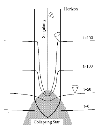
Figure 1: A spacetime diagram showing the formation of a BH, and time slices traditionally used to foliate the spacetime in traditional numerical relativity with singularity avoiding time slices. As the evolution proceeds, pathologically warped hypersurfaces develop, leading to unresolvable gradients that cause numerical codes to crash.

2.5.1 Apparent Horizon Boundary Conditions (AHBC)

The cosmic censorship conjecture suggests that in physical situations, singularities are hidden inside BH horizons. Because the region of spacetime inside the horizon is causally disconnected from the region of interest outside the horizon, one is tempted numerically to cut away the interior region containing the singularity, and evolve only the singularity-free region outside, as originally suggested by Unruh[85]. This has the consequence that there will be a region inside the horizon that simply has no numerical data. To an outside observer no information will be lost since the regions cut away are unobservable. Because the time slices will not need such sharp bends to the past, this procedure will drastically reduce the dynamic range, making it easier to maintain accuracy and stability. Since the singularity is removed from the numerical spacetime, there is in principle no physical reason why BH codes cannot be made to run indefinitely without crashing.

We spoke innocently about the BH horizon, but did not distinguish between the apparent and event horizon. These are very different concepts! While the event horizon, which is roughly a null surface that never reaches infinity and never hits the singularity, may hide singularities from the outside world in many situations, there is no guarantee that the apparent horizon, which is the (outermost) surface that has instantaneously zero expansion everywhere, even exists on a given slice! (By “zero expansion” we mean that the surface area of outgoing bundles of photons normal to the surface is constant. Hence, the surface is “trapped.”) Methods for finding event horizons in numerical spacetimes are now known, and will be discussed below. But event horizons can only be found after examining the history of an evolution that has been already been carried out to sufficiently late times[86, 87]. Hence they are useless in providing boundaries as one integrates forward in time. On the other hand the apparent horizon, if it exists, can be found on any given slice by searching for closed 2–surfaces with zero expansion. Although one should worry that in a generic BH collision, one may evolve into situations where no apparent horizon actually exists, let us cross that bridge if we come to it. Methods for finding apparent horizons will also be discussed below, but for now we assume that such a method exists.

Given these considerations, there are two basic ideas behind the implementation of the apparent horizon boundary condition (AHBC), also known as black hole excision:

(a) It is important to use a finite differencing scheme which respects the causal structure of the spacetime. Since the horizon is a one-way membrane, quantities on the horizon can be affected only by quantities outside but not inside the horizon: all quantities on the horizon can in principle be updated solely in terms of known quantities residing on or outside the horizon. There are various technical details and variations on this idea, which is called “Causal Differencing”[88] or “Causal Reconnection”[89], but here we focus primarily on the basic ideas and results obtained to date.

(b) A shift is used to control the motion of the horizon, and the behavior of the grid points outside the BH, as they tend to fall into the horizon if uncontrolled.

An additional advantage to using causal differencing is that it allows one to follow the information flow to create grid points with proper data on them, as needed inside the horizon, even if they did not exist previously. (Remember above that we have cut away a region inside the horizon, so in fact we have no data there.) One example is to let a BH move across the computational grid. If a BH is moving physically, it may also be desirable to have it move through coordinate space. Otherwise, all physical movement will be represented by the “motion” of the grid points. For a single BH moving in a straight line, this may be possible (though complicated), but for spiraling coalescence this will lead to hopelessly contorted grids. The immediate consequence of this is that as a BH moves across the grid, regions in the wake of the hole, now in its exterior, must have previously been inside it where no data exist! But with AHBC and causal differencing this need not be a problem.

Does the AHBC idea work? Preliminary indications are very promising. In spherical symmetry (1D), numerous studies show that one can locate horizons, cut away the interior, and evolve for essentially unlimited times ($t\propto 10^{3-4}M$, where $M$ is the black hole mass). The growth of metric functions can be completely controlled, errors are reduced to a very low level, and the results can be obtained with a large variety of shift and slicing conditions, and with matter falling in the BH to allow for true dynamics even in spherical symmetry[88, 90, 91, 92].

In 3D, the basic ideas are similar but the implementation is much more difficult. The first successful test of these ideas to a Schwarzschild BH in 3D used horizon excision and a shift provided from similar simulations carried out with a 1D code[42]. The errors were found to be greatly reduced when compared even to the 1D evolution with singularity avoiding slicings. Another 3D implementation of the basic technique was provided by Brügmann [46].

This was a proof of principle, but more general treatments are following. Daues extended this work to a full range of shift conditions [3], including the full 3D minimal distortion shift [7]. He also applied these techniques to dynamic BH’s, and collapse of a star to form a BH, at which point the horizon is detected, the region interior to the horizon excised, and the evolution continued with AHBC. The focus of this work has been on developing general gauge conditions for single BH’s without movement through a grid. Under these conditions, BH’s have been accurately evolved well beyond $t=100M$. The NSF Black Hole Grand Challenge Alliance had focussed on development of 3D AHBC techniques for moving Schwarzschild BH’s[4]. In this work, analytic gauge conditions are provided, which are chosen to make the evolution static, although the numerical evolution is allowed to proceed freely. This moving hole is the first successful 3D test of populating grid points with data as they emerge in the BH wake.

These new results are significant achievements, and show that the basic techniques outlined above are not only sound, but are also practically realizable in a 3D numerical code. However, there is still a significant amount of work to be done! The techniques have yet to be applied carefully to distorted BH’s, with tests of the waveforms emitted. They have not been applied to rotating BH’s of any kind; they have not been applied to colliding BH’s with horizon topology change, and moving black holes have yet to be evolved in AHBC with a nonanalytic gauge choice. There are still clearly many steps to be taken before the techniques will be successfully applied to the general BH merger problem.

3 Tools for Analyzing the Numerical Spacetimes

We now turn to the description of several important tools that have been developed to analyze the results of a numerical evolution, carried out by some numerical evolution scheme. The evolution will generally provide metric functions on a grid, but as described above these functions are highly dependent on both the coordinate system and gauge in which the system is evolved. Determining physical information, such as whether a black hole exists in the data, or what gravitational waveforms have been emitted, are the subjects of this section.

3.1 Horizon Finders

As described above, black holes are defined by the existence of an event horizon (EH), the surface of no return from which nothing, not even light, can escape. The event horizon is the boundary that separates those null geodesics that reach infinity from those that do not. The global character of such a definition implies that the position of an EH can only be found if the whole history of the spacetime is known. For numerical simulations of black hole spacetimes in particular, this implies that in order to locate an EH one needs to evolve sufficiently far into the future, up to a time where the spacetime has basically settled down to a stationary solution. Recently, methods have been developed to locate and analyze black hole horizons in numerically generated spacetimes, with a number of interesting results obtained [86, 87, 93, 94, 95, 96].

In contrast, an apparent horizon (AH) is defined locally in time as the outer-most marginally trapped surface [97], i.e. a surface on which the expansion of out-going null geodesics is everywhere zero. An AH can therefore be defined on a given spatial hypersurface. A well known result [97] guarantees that if an AH is found, an EH must exist somewhere outside of it and hence a black hole has formed.

3.2 Locating the apparent horizons

The expansion $\Theta$ of a congruence of null rays moving in the outward normal direction to a closed surface can be shown to be [17]

$$\Theta=\nabla_{i}s^{i}+K_{ij}s^{i}s^{j}-{\rm tr}K,$$ (17)

where $\nabla_{i}$ is the covariant derivative associated with the 3-metric $\gamma_{ij}$, $s^{i}$ is the normal vector to the surface, $K_{ij}$ is the extrinsic curvature of the time slice, and ${\rm tr}K$ is its trace. An AH is then the outermost surface such that

$$\Theta=0.$$ (18)

This equation is not affected by the presence of matter, since it is purely geometric in nature. We can use the same horizon finders without modification for vacuum as well as non-vacuum spacetimes. The key is to find a closed surface with normal vector $s^{i}$ satisfying this equation.

3.2.1 Minimization Algorithms

As apparent horizons are defined by the vanishing of the expansion on a surface, a fairly obvious algorithm to find such a surface involves minimizing a suitable norm of the expansion below some tolerance while adjusting test surfaces. Minimization algorithms for finding apparent horizons were among the first methods developed [98, 99]. More recently, a 3D minimization algorithm was developed and implemented by the Potsdam/NCSA/WashU group, applied to a variety of black hole initial data and 3D numerically evolved black hole spacetimes [100, 101, 102, 103, 104]. Essentially the same algorithm was also implemented independently by Baumgarte et.al. [105].

The basic idea behind a minimization algorithm is to assume the surface can be represented by a function $F(x^{i})=0$, expand it the in terms of some set of basis functions, and then minimize the integral of the square of the expansion $\Theta^{2}$ over the surface. For example, one can parameterize a surface as

$$F(r,\theta,\phi)=r-h(\theta,\phi).$$ (19)

The surface under consideration will be taken to correspond to the zero level of $F$. The function $h(\theta,\phi)$ is then expanded in terms of spherical harmonics:

$$h(\theta,\phi)=\sum_{l=0}^{l_{\rm max}}\sum_{m=-l}^{l}a_{lm}Y_{lm}(\theta,\phi).$$ (20)

Similar techniques were developed by [106].

At an AH the expansion integral over the surface should vanish, and we will have a global minimum. Of course, since numerically we will never find a surface for which the integral vanishes exactly, one must set a given tolerance level below which a horizon is assumed to have been found.

Minimization algorithms for finding AH’s have a few drawbacks: First, the algorithm can easily settle down on a local minimum for which the expansion is not zero, so a good initial guess is often required. Moreover, when more than one marginally trapped surface is present, as is often the case, it is very difficult to predict which of these surfaces will be found by the algorithm: The algorithm can often settle on an inner horizon instead of the true AH. Again, a good initial guess can help point the finder towards the correct horizon. Finally, minimization algorithms tend to be very slow when compared with ‘flow’ algorithms of the type described in the next section. Typically, if $N$ is the total number of terms in the spectral decomposition, a minimization algorithm requires of the order of a few times $N^{2}$ evaluations of the surface integrals (where in our experience ‘a few’ can sometimes be as high as 10).

This algorithm has been implemented in the “Cactus” code for 3D numerical relativity [31]. For more details of the application of this algorithm, see Refs. [100, 101, 105, 102].

3.2.2 3D fast flow algorithm

A second method that has been implemented in the “Cactus” code is the “fast flow” method proposed by Gundlach [107]. Starting from an initial guess for the $a_{lm}$, it approaches the apparent horizon through the iteration

$$a_{lm}^{(n+1)}=a_{lm}^{(n)}-{A\over 1+Bl(l+1)}\left(\rho\Theta\right)_{lm}^{(n)}.$$ (21)

where $(n)$ labels the iteration step, $\rho$ is some positive definite function (“a weight”), and $(\rho\Theta)_{lm}$ are the harmonic components of the function $(\rho\Theta)$. Various choices for the weight $\rho$ and the coefficients $A$ and $B$ parameterize a family of such methods. The fast flow algorithm in Cactus uses

$$\rho=2\;r^{2}|\nabla F|\left[\left(g^{ij}-s^{i}s^{j}\right)\left(\bar{g}_{ij}-\nabla_{i}r\nabla_{j}r\right)\right]^{-1},$$ (22)

where $\bar{g}_{ij}$ is the flat background metric associated with the coordinates $(r,\theta,\phi)$, and

$$A={\alpha\over l_{\rm{max}}(l_{\rm{max}}+1)}+\beta,\quad B={\beta\over\alpha}.$$ (23)

with $\alpha=c$ and $\beta=c/2$. Here $c$ is a variable step size, with a typical value of $c\sim 1$. $l_{\rm{max}}$ is the maximum value of $l$ one chooses to use in describing the surface. The iteration procedure is a finite difference approximation to a parabolic flow, and the adaptive step size is chosen to keep the finite difference approximation roughly close to the flow limit to prevent overshooting of the true apparent horizon. The adaptive step size is determined by a standard method used in ODE integrators: we take one full step and two half steps and compare the resulting $a_{lm}$. If the two results differ too much one from another, the step size is reduced.

Other methods for finding apparent horizons, based directly on computing the jacobian of the finite differenced horizon equation, have been developed[108, 109] and successfully used in 3D. For details, please see these references.

3.3 Locating the event horizons

The AH is defined locally in time and hence is much easier to locate than the event horizon (EH) in numerical relativity. The EH is a global object in time; it is traced out by the path of outgoing light rays that never propagate to future null infinity, and never hit the singularity. (It is the boundary of the causal past of future null infinity $\dot{\cal{J}}^{{-}}(\cal{I}^{+})$.) In principle one needs to know the entire time evolution of a spacetime in order to know the precise location of the EH. However, in spite of the global properties of the EH, hope is not lost for finding it very accurately, even in a numerical simulation of finite duration. Here we discuss a method to find the EH, given a numerically constructed black hole spacetime that eventually settles down to an approximately stationary state at late times. In principle, as the EH is a null surface, it can be found by tracing the path of null rays through time. Outward going light rays emitted just outside the EH will diverge away from it, escaping to infinity, and those emitted just inside the EH will fall away from it, towards the singularity. In a numerical integration it is difficult to follow accurately the evolution of a horizon generator forward in time, as small numerical errors cause the ray to drift and diverge rapidly from the true EH. It is a physically unstable process. But we can actually use this property to our advantage by considering the time-reversed problem. In a global sense in time, any outward going photon that begins near the EH will be attracted to the horizon if integrated backward in time [86, 100]. In integrating backwards in time, it turns out that it suffices to start the photons within a fairly broad region where the EH is expected to reside. Such a horizon-containing region, as we call it, is often easy to determine after the spacetime has settled down to approximate stationarity. The crucial point is that when integrated backward in time along null geodesics, this horizon-containing region shrinks rapidly in “thickness”, leading to a very accurate determination of the location of the EH at earlier times. Note that it is the earlier time when the black hole is under highly dynamical evolution that we are really interested in.

Although one can integrate individual null geodesics backward in time, we find that there are various advantages to integrate the entire null surface backward in time. A null surface, if defined by $f(t,x^{i})=0$ satisfies the condition

$$g^{\mu\nu}\partial_{\mu}f\partial_{\nu}f=0\;.$$ (24)

Hence the evolution of the surface can be obtained by a simple integration,

$$\partial_{t}f=\frac{-g^{ti}\partial_{i}f+\sqrt{(g^{ti}\partial_{i}f)^{2}-g^{tt}g^{ij}\partial_{i}f\partial_{j}f}}{g^{tt}}\;.$$ (25)

The inner and outer boundary of the horizon containing region when integrated backward in time, will rapidly converge to practically a single surface to within the resolution of the numerically constructed spacetime, i.e., a small fraction of a grid point. An accurate location of the event horizon is hence obtained. We henceforth shall represent the horizon surface as the function $f_{H}(t,x^{i})$. Aside from the simplicity of this method, there are a number of technical advantages as discussed in [86]. One particularly noteworthy point is that this method is capable of giving the caustic structure of the event horizon if there is any; for details see [86].

The function $f_{H}(t,x^{i})$ provides the complete coordinate location of the EH through the spacetime (or a very good approximation of it, as shown in [87]). This function by itself directly gives us the topology and location of the EH. When combined with the induced metric function on the surface, which is recorded throughout the evolution, it gives the intrinsic geometry of the EH. When further combined with the spacetime metric, all properties of the EH including its embedding can be obtained. Moreover, as the normal of $f_{H}(t,x^{i})=0$ gives the null generators of the horizon, it is an easy further step to determine the null generators, and hence the complete dynamics of the horizon in this formulation.

As described in a series of papers, the event horizon, once found with such a method, can be analyzed to provide important information about the dynamics of black holes in a numerically generated spacetime [86, 87, 93, 94, 95, 96].

3.4 Wave Extraction

The gravitational radiation emitted is one of the most important quantities of interest in many astrophysical processes. The radiation is generated in regions of strong and dynamic gravitational fields, and then propagated to regions far away where it will someday be detected. We take the approach of computing the generation and evolution of the fields in a fully nonlinear way, while analyzing the radiation with a perturbation formulation in the regions where it can be so treated.

The theory of black hole perturbations is well developed. One identifies certain perturbed metric quantities that evolve according to wave equations on the black hole background. These perturbed metric functions are also dependent of the gauge in which they are computed. We use a gauge-invariant prescription for isolating wave modes on black hole background, developed first by Moncrief [110]. The basic idea is that although the perturbed metric functions transform under coordinate transformations (gauge transformations), one can identify certain linear combinations of these functions that are invariant to first order of the perturbation. These gauge-invariant functions are the quantities that carry true physics, which does not depend on coordinate systems. They obey the wave equations describing waves propagating on the fixed blackhole background. There are two independent wave modes, even- and odd-parity, corresponding to the two degrees of freedom, or polarization modes, of the waves.

A waveform extraction procedure has been developed that allows one to process the metric and to identify the wave modes. The gravitational wave function (often called the “Zerilli function” for even-parity or the “Regge-Wheeler function” for odd-parity) can be computed by writing the metric as the sum of a background black hole part and a perturbation:

$$g_{\alpha\beta}=\stackrel{{\scriptstyle o}}{{g}}_{\alpha\beta}+h_{\alpha\beta}(Y_{\ell,m}),$$ (26)

where the perturbation $h_{\alpha\beta}$ is expanded in spherical harmonics and their tensor generalizations and the background part $\stackrel{{\scriptstyle o}}{{g}}_{\alpha\beta}$ is spherically symmetric. To compute the elements of $h_{\alpha\beta}$ in a numerical simulation, one integrates the numerically evolved metric components $g_{\alpha\beta}$ against appropriate spherical harmonics over a coordinate 2–sphere surrounding the black hole, making use of the orthogonality properties of the tensor harmonics. This process is performed for each $\ell,m$ mode for which waveforms are desired. The resulting functions $h_{\alpha\beta}(Y_{\ell,m})$ can then be combined in a gauge-invariant way, following the prescription given by Moncrief[110]. For each $\ell,m$ mode, this gauge invariant gravitational waveform can be extracted when the wave passes through “detectors” at some fixed radius in the computational grid. This procedure has been described in detail in [111, 112, 113], and more generally in Refs. [114, 115, 104]. It works amazingly well, allowing extraction of waves that carry very small energies (of order $10^{-7}M$ or less, with $M$ being the mass of the source) away from the source. The procedure should apply to any isolated source of waves, such as colliding black holes, neutron stars, etc. If the sources are rotating, this procedure should be generalized to use the Teukolsky formalism describing perturbations about a Kerr black hole, but this has not yet been done. Instead, the spherical perturbation theory (with a few minor modifications) has been applied to distorted rotating black holes with satisfactory results [111, 112, 113].

4 Computational Science, Numerical Relativity, and the “Cactus” Code

4.1 The Computational Challenges of Numerical Relativity

Before we describe our computational methods in the following subsections, we summarize the computational challenges of numerical relativity discussed above. It is in response to these challenges that we have devised the computational methods.

$\bullet$ Computational challenges due to the complexity of the physics involved: The Einstein equations are probably the most complex partial differential equations in all of physics, forming a system of dozens of coupled, nonlinear equations, with thousands of terms, of mixed hyperbolic, elliptic, and even undefined types in a general coordinate system. The evolution has elliptic constraints that should be satisfied at all times. In simulations without symmetry, as would be the case for realistic astrophysical processes, codes can involve hundreds of 3D arrays, and ten of thousands of operations per grid point per update. Moreover, for simulations of astrophysical processes, we will ultimately need to integrate numerical relativity with traditional tools of computational astrophysics, including hydrodynamics, nuclear astrophysics, radiation transport and magneto-hydrodynamics, which govern the evolution of the source terms (i.e., the right hand side) of the Einstein equations. This complexity requires us to push the frontiers of massively parallel computation.

$\bullet$ Challenge in Collaborative Technology: The integration of numerical relativity into computational astrophysics is a multi-disciplinary development, partly due to the complexity of the Einstein equations, and partly due to the physical systems of interest. Solving the Einstein equations on massively parallel computers involves gravitational physics, computational science, numerical algorithm and applied mathematics. Furthermore, for the numerical simulations of realistic astrophysical systems, many physics disciplines, including relativity, astrophysics, nuclear physics, and hydrodynamics are involved. It is therefore essential to have the numerical code software engineered to allow co-development by different research groups and groups with different expertise.

$\bullet$ The numerical construction of a spacetime itself presents unique challenges: According to the singularity theorems of general relativity, regions of strong gravity often generate spacetime singularities. Due to the need to avoid spacetime singularities [24, 116], and to obtain long term stability in the numerical simulations, sophisticated control of the coordinate system is needed for the construction of a numerical spacetime. This dynamic interplay between the spacetime being constructed and the computational coordinate choice itself (“gauge choice”) is a unique feature of general relativity that makes the numerical simulations much more demanding. Besides extra computational power, advanced visualization tools, preferably real time interactive “window into the oven” visualization, are particularly useful in the numerical construction.

$\bullet$ The multi-scale problem: Astrophysics of strongly gravitating systems inherently involves many length and time scales. The microphysics of the shortest scale (the nuclear force), controls macroscopic dynamics on the stellar scale, such as the formation and collapse of neutron stars (NSs). On the other hand, the stellar scale is at least 10 times less than the wavelength of the gravitational waves emitted, and many orders of magnitude less than the astronomical scales of their accretion disk and jets; these larger scales provide the directly observed signals. Numerical studies of these systems, aiming at direct comparison with observations, fundamentally require the capability of handling a wide range of dynamical time and length scales.

All of these issues lead to important research questions in computational science. Here we give an overview of some of our effort in these directions, focusing on performance and coding issues on parallel machines, and on the development of a community code that incorporates all the mathematical and computational techniques described above (and many more), in a collaborative infrastructure for numerical relativity.

4.2 Code Generation and Data Parallel Fortran

When expanded out in a particular coordinate system the evolution equations for the full Einstein equations in the 3$+$1 formulation have many thousands of terms. These are usually derived and coded in Fortran with a symbolic manipulator package such as Mathematica or Macsyma. However, these packages often generate Fortran expressions that are unsuitable for most compilers, even on traditional supercomputers. We often exceed internal compiler limits on length of expression, number of continuation lines, number of arguments to a subroutine, number of nested parentheses, and so forth. So our code generation techniques need to be carefully massaged before an efficient, working code is generated.

The evolution equations are generally written out using explicit finite difference schemes, which are very popular for hyperbolic systems of equations. These equations are good candidates for the “SIMD” style approach to programming parallel machines. (SIMD stands for “Single Instruction Multiple Data”, which means an operation like “add arrays A and B together” can be carried out completely in parallel, with the same instruction (add) on multiple data elements in memory. This is also a so-called “data parallel” operation, since the same operation is applied simultaneously to all data elements of arrays A and B in parallel, and no communications are required between processors.) Until recently, in our research group 3D codes have been generally written in this style using data parallel Fortran90 and CMFortran style languages. With this approach, communications between processors, required for example when computing derivatives (which require knowledge of neighboring data points in memory), are handled by the compilers without need for the user to do anything. We have used the C-preprocessor to incorporate a few different code blocks so that we can maintain a single source file for several machines. (For an excellent review of many modern approaches to parallel computing, including further information on many of the concepts and acronyms common in computational science, see, e.g., [117], available both in print and on-line).

Using this global approach we previously developed a single code, called H3expresso, that achieved over 15 Gflops on the 512 node CM-5 and about 8 Gflops on the 16 processor Cray C-90. This code was one of the fastest applications on either machine [118]. We performed a detailed comparative study of this code on many architectures, including the C-90, Convex SPP-1200, T3D, CM-5, SGI Power Challenge, and SP-2, achieving excellent scaling all machines. These results are possible because of the very high computation/communication ratio inherent in the Einstein equations. The hyperbolic equations contain thousands of terms to be evaluated, while the only communications required are in computing finite differences for numerical derivatives.

4.3 Data Parallel Fortran Evolves to MPI

However, this data parallel approach is not the best one to follow with more modern microprocessor based scalable supercomputers, such as the SGI/Cray Origin 2000 and Cray T3D and T3E, due largely to the use of caches that boost performance of a single node. It is worth commenting on how we have adapted the H3expresso code to a “message passing” language like MPI, with single processor optimizations, which then led to to the development of the new Cactus code described below. (MPI stands for “Message Passing Interface”, a standard communications library now available on most parallel computers, that allows the user to explicitly control the communication of data between processors when required [117]. This can be more efficient than allowing the compiler to handle this automatically.)

Due to the data-parallel nature of the code, many of the temporaries evolved in solving the hyperbolic equations (11), notably the sources and the fluxes, are created as 3D arrays. This allows fairly easy parallelization of the code with MPI. Since the only finite differencing in the code is on the fluxes, they are the only variables which need communication, and thus we can easily do an MPI-based communication with these variables during our update loop.

Unfortunately, one of the major problems of the data parallel programming model is that it requires the creation of large numbers of 3D temporary arrays to store source or flux terms. On a system like the CM-5, this technique was crucial in obtaining performance; the arrays were distributed and were stored on the vector units, so the system could operate on them quickly and communicate them transparently. However, with single statements for entire arrays with large degrees of complexity, each assignment requires a sweep through the complete memory space. Cache locality is impossible, and the code performs very poorly in an out-of-cache regime. Hence, to achieve high single processor performance on more modern microprocessor based architectures special attention has to be paid to rewriting expressions to maximize the use of the processor cache.

Using the experience gained from exploring issues of parallelism and single processor performance with the H3expresso code, we have developed from the scratch a new 3D Einstein equation code, the “Cactus” code, which integrates important design decisions for modern HPC (standard acronym for “High Performance Computing”) architectures from the outset:

• The numerical kernals for the Einstein equations, needed by all users, are highly optimized for modern microprocessor based architecture.

• Other routines (e.g., waveform extraction) are written by the community of users in either C or Fortran.

• It obtains parallelism through MPI, not through compiler technologies. In the following, we describe some details of single processor performance, parallelism and the code’s collaborative infrastructure.

4.3.1 Parallelism using MPI

In “Cactus”, we achieve parallelism using ghost-zone domain decomposition. That is, we decompose a global domain over our processors, and place an overlap region on each processor. Then each single processor is responsible for updating the interior of their local region, and a MPI communication synchronizes the boundary zones after communications. We have also optimized for the particular structure of our equations. The straightforward way to set up our communication patterns would be an algorithm like

  for (it = 0 to maxit) {
    update interior for a time step dt
    update ghost zones for all grid functions
  }

However, many of our variables have no flux. Since we generally use a strang split in the hyperbolic evolution, which allows us to update our source and flux evolution separately, the integration of these flux-free variables is a completely spatially de-coupled point local ODE. These variables need no communication whatsoever, in absence of flux. Thus, we can re-write the above loop as

  for (it = 0 to maxit) {
    evolve sources for dt/2
    evolve fluxes for dt
    update ghost zones for all grid functions which have a flux
    evolve sources for dt/2
  }

In practice, this algorithm allows us to reduce our communication cost, resulting in excellent scaling, in addition to excellent single processor performance.

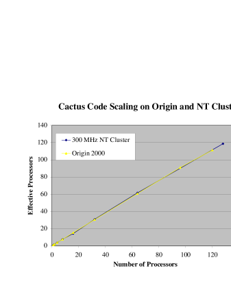
Figure 2: We show scaling of the Cactus code on two very different architectures: an SGI/Cray Origin 2000 DSM architecture with 128 processors, and a cluster of 300Mhz Compaq workstations running Windows NT. The data is obtained with all ”thorns” that are needed to evolve a gravitational wave packet using the vacuum Einstein equation.

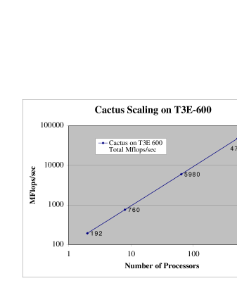
Figure 3: We show the scaling of the Cactus code on the Cray T3E-600, giving the total Mflops/sec as a function of the number of processors. Results are shown for single precision calculations, and include calculations performed on ghost zones. The grid size per processor is kept constant as the number of processors in increased (so the total problem size scales with the size the machine). The performance data is obtained for an evolution using the Einstein equations with the hydrodynamic source terms, and the relativistic hydrodynamics equations in high resolution shock capturing treatment as described in the paper. The inclusion of the hydrodynamics does not change the performance in any substantial manner.

These techniques have enabled “Cactus” to be a highly portable and efficient code for numerical relativity and astrophysics. It has been tested and performed very well on three very different parallel architectures: the SGI Origin 2000 system, the SGI/Cray T3E system, and a cluster of 128 NT workstations, developed at NCSA, running Pentium II processors. In Fig. 3 we show scaling results achieved on a Cray T3E-600, and in Fig. 2 we show the scaling results achieved on both the Origin 2000 and the NT cluster. Presently, the SGI Origin, with 250MHz R10000 processors, has more than three times the per processor performance of the 300MHz Pentium II in the NT cluster, but the trend is very encouraging. These results indicate that codes like this can be run efficiently in parallel on a wide variety of machines.

Finally, we have recently tested the code on a 1024 node T3E-1200 (provided for the NASA Neutron Star Grand Challenge Project [76] for performance tests), achieving 142GFlops and linear scaling up to 1024 nodes. The version of the code tested is the so-called GR3D code developed for the NASA Grand Challenge Project. GR3D is a version of “Cactus” code for spacetime evolution coupled to a Riemann solver based relativistic hydrodynamic code (MAHC HYPERBOLIC_HYDRO) that has recently been released (available at http://wugrav.wustl.edu/Codes/GR3D/). Performance information for the “Cactus” code will also be kept up to date at http://cactus.aei-potsdam.mpg.de.

In the following we give a summary of the performance test. The test was carried out with the released version without special tuning for this 1024 node machine. We note that the full set of the Einstein equations with the perfect fluid source, as solved in this code, involved a large number of 3D arrays. The huge number of grid points used (644 x 644 x 1284, or 500 x 500 x 996 respectively for 32 and 64 bits) is made possible by reduced memory footprint of the code.

Machine Configuration: 1024 node T3E-1200 with 512MB per node

Date tested: May 10, 1998

                                  32 bit             64 bit
--------------------------------------------------------------------
Grid Size per Processor           84x84x84           66x66x66
Processor topology                8 x8 x16           8 x8 x16
Total Grid Size                   644 x 644 x 1284   500 x 500 x 996
Single Proc MFlop/sec             144.35             118.33
Aggregate GFlop/sec               142.2              115.8
Scaling efficiency                96.2\%              95.6\%
--------------------------------------------------------------------

Previously, the largest production simulations in 3D numerical relativity have been limited to about $300^{3}$ or less, and applied to distorted 3D black hole systems [119, 104, 114, 115]. When such large machines as the test T3E described above are made available for routine production simulations, we expect to further improve the results of the such black hole simulations, and perform more general 3D calculations involving distorted rotating black holes, coalescences of neutron stars, gravitational waves, as well as other interesting problems in general relativistic astrophysics.

4.4 Collaborative Infrastructure

While “Cactus” is our third generation 3D numerical relativity code, it is our first generation of code in which we paid special attention to the difficult software engineering problem of collaborative code development, maintenance and management. Our earlier generations of 3D numerical relativity codes (the so-called “G” and “H” codes, described in [42, 120]) involving about a dozen researchers in the Potsdam/NCSA/Wash U collaboration, have made us keenly aware of the issues and difficulties involved in distributed collaborative code development. For the “Cactus” code, a collaborative infrastructure has been essential. As of this writing, several dozen collaborators at 7 institutions are using the code for various research projects, and we aim at further making it a truly community code for the investigation of general relativistic astrophysics.

“Cactus” is hence designed to minimize barriers to the community development and use of the code, including the complexity associated with both the code itself and the networked supercomputer environments in which simulations and data analyses are performed. This complexity is particularly noticeable in large multidisciplinary simulations such as ours, because of the range of disciplines that must contribute to code development (relativity, hydrodynamics, astrophysics, numerics, and computer science) and because of the geographical distribution of the people and computer resources involved in simulation and data analysis.

The collaborative technologies that we are developing within Cactus include:

$\bullet$ A modular code structure and associated code development tools. Cactus defines coding rules that allow one, with only a working knowledge of Fortran or C, to write new code modules that are easily plugged in as “thorns” to the main Cactus code (the “flesh”). The “flesh” contains basic computational infrastructure needed to develop and connect parallel modules into a working code. All told, the “flesh” is thousands of lines of highly optimized C and Fortran, not counting some utility libraries, makefile, and perl scripts. It allows one to plug in not only different physics modules, such as the basic Einstein solver, other formulations of the equations, analysis routines, etc., but also different parallel domain decomposition modules, I/O modules, utilities, elliptic solvers, and so forth. A thorn may be any code that the user wants, in order to provide different initial data, different matter fields, different gauge conditions, visualization modules, etc. Thorns need not have anything to do with relativity: the flesh could be used as basic infrastructure for any set of PDE’s, from Newtonian hydrodynamics equations to Yang Mills equations, that are coded as thorns. The user inserts the hook to their thorn into the flesh code in a way that the thorn will not be compiled unless it is designated to be active. We have developed a makefile and perl-based thorn management system that, through the use of preprocessor macros that are appropriately expanded to the arguments of the flesh and additional arguments defined by each thorn, is able to create a code which can configure itself to have a variety of different modules. This ensures that only those variables needed for a particular simulation are actually used, and that no conflicts can be created in subroutine argument calling lists.

$\bullet$ A consistency test suite library. An increased number of thorns makes the code more attractive to its community but also increases the risk of incompatibilities. Hence, we provide technology that allows each developer to create a test/validation suite for their own thorn. These tests are run prior to any check in of code to the repository, ensuring that new code reproduces results consistent with previous one, and hence cannot compromise the work of other developers relying on a given thorn.

So, how does a user use the code? A detailed user guide will be available with the code when it is released during 1999 (see http://cactus.aei-potsdam.mpg.de), but in a nutshell, one specifies which physics modules, and which computational/parallelism modules, are desired in a configuration file, and makes the code on the desired architecture, which can be any one of a number of machines from SGI/Cray Origin or T3E, Dec Alpha, Linux workstations or clusters, NT clusters, and others. The make system automatically detects the architecture and configures the code appropriately. Control of run parameters is then provided through an input file. Additional modules can be selected from a large community-developed library, or new modules may be written and used in conjunction with the pre-developed modules.

Our experiences with Cactus up to now suggest that these techniques are effective. It allows a code of many tens of thousands of lines, but with a compact flesh that is possible to maintain despite the large number of people contributing to it. The common code base has enhanced the collaborative process, having important and beneficial effects on the flow of ideas between remote groups. This flexible, open code architecture allows, for example, a relativity expert to contribute to the code without knowing the details of, say, the computational layers (e.g., message passing or AMR libraries) or other components (e.g., hydrodynamics). This is an area that we plan to invest more effort into in the coming few years.

4.5 Adaptive Mesh Refinement

3D simulations of Einstein’s equations are very demanding computationally. In this section we outline the computational needs, and techniques designed to reduce them. We will need to resolve waves with wavelengths of order $5M$ or less, where $M$ is the mass of the BH or the neutron star. Although for Schwarzschild black holes, the fundamental $\ell=2$ quasinormal mode wavelength is $16.8M$, higher modes, such as $\ell=4$ and above, have wavelengths of $8M$ and below. The BH itself has a radius of $2M$. More important, for very rapidly rotating Kerr BH’s, which are expected to be formed in realistic astrophysical BH coalescence, the modes are shifted down to significantly shorter wavelengths[2, 1]. As we need at least 20 grid zones to resolve a single wavelength, we can conservatively estimate a required grid resolution of about $\Delta x=\Delta y=\Delta z\approx 0.2M$. For simulations of time scales of order $t\propto 10^{2}-10^{3}M$, which will be required to follow coalescence, the outer boundary will probably be placed at a distance of roughly $R\propto 100M$ from the coalescence, requiring a Cartesian simulation domain of about $200M$ across. This leads to about $10^{3}$ grid zones in each dimension, or about $10^{9}$ grid zones in total. As 3D codes to solve the full Einstein equations have typically 100 variables to be stored at each location, and simulations are performed in double precision arithmetic, this leads to a memory requirement of order 1000 Gbytes! (In fairness to some groups that use spectral methods instead of finite differences (e.g., the Meudon group), we should point out highly accurate 3D simulations can now be achieved on problems that are well suited to such techniques, using much less memory! [121]).

The largest supercomputers available to scientific research communities today have only about $\frac{1}{20}$ of this capacity, and machines with such capacity will not be routinely available for some years. Furthermore, if one needs to double the resolution in each direction for a more refined simulation, the memory requirements increase by an order of magnitude. Although such estimates will vary, depending on the ultimate effectiveness of inner or outer boundary treatments, gauge conditions, etc., they indicate that barring some unforeseen simplification, some form of adaptive mesh refinement (AMR) that places resolution only where it is required is not only desirable, but essential. The basic idea of AMR is to use some set of criteria to evaluate the quality of the solution on the present time step. If there are regions that require more resolution, then data are interpolated onto a finer grid in those regions; if less resolution is required, grid points are destroyed. Then the evolution proceeds to the next time step on this hierarchy of grids, where the process is repeated. These rough ideas have been refined and applied in many applications now in computational science.

There are several efforts ongoing in AMR for relativity. Choptuik was the early pioneer in this area, developing a 1D AMR system to handle the resolution requirements needed to follow scalar field collapse to a BH[122]. As an initially regular distribution of scalar field collapses, it will require more and more resolution as its density builds up. The grid density required to resolve the initial distribution may not even see the final BH. Further, as pulses of radiation propagate back out from the origin, they, too may have to be resolved in regions where there was previously a coarse grid. Choptuik’s AMR system, built on early work of Berger and Oliger[123], was able to track dynamically features that develop, enabling him to discover and accurately measure BH critical phenomena that have now become so widely studied[124].

Based on this success and others, and on the general considerations discussed above, full 3D AMR systems are under development to handle the much greater needs of solving the full set of 3D Einstein equations. A large collaboration, begun by the NSF Black Hole Grand Challenge Alliance, has been developing a system for distributing computing on large parallel machines, called Distributed Adapted Grid Hierarchies, or DAGH. DAGH was developed to provide MPI-based parallelism for the kinds of computations needed for many PDE solvers, and it also provides a framework for parallel AMR. It is one of the major computational science accomplishments to come out of the Alliance. Developed by Manish Parashar and Jim Browne, in collaboration with many subgroups within and without the Alliance, it is now being applied to many problems in science and engineering. One can find information about DAGH online at http://www.cs.utexas.edu/users/dagh/.

At least two other 3D software environments for AMR have been developed for relativity: one is called HLL, or Hierarchical Linked Lists, developed by Lee Wild and Bernard Schutz[125]; another, called BAM, was the first AMR application in 3D relativity developed by Brügmann [46]. The HLL system has recently been applied to the test problem of the Zerilli equation (discussed above) describing perturbations of black holes[126]. This nearly 30 year old linear equation is still providing a powerful model for studying BH collisions, and it is also being used as a model problem for 3D AMR. In this work, the 1D Zerilli equation is recast as a 3D equation in cartesian coordinates, and evolved within the AMR system provided by HLL. Even though the 3D Zerilli equation is a single linear equation, it is quite demanding in terms of resolution requirements, and without AMR it is extremely difficult to resolve both the initial pulse of radiation, the blue shifting of waves as they approach the horizon, and the scattering of radiation, including the normal modes, far from the hole.

5 Summary

In this article we have attempted to review the essential mathematical and computational elements needed for a full scale numerical relativity code that can treat a variety of problems in relativistic astrophysics and gravitation. Various formulations of the Einstein equations for evolving spacelike time slices, techniques for providing initial data, the basic ideas of gauge conditions, several important analysis tools for discovering the physics contained in a simulation, and numerical algorithms for each of these items have been reviewed. Unfortunately, we have only been able to cover the basics of such a program, and in addition many promising alternative approaches have necessarily been left out.

As one can see, the solution to a single problem in numerical relativity requires a huge range of computational and mathematical techniques. It is truly a large scale effort, involving experts in computer and computational science, mathematical relativity, astrophysics, and so on. For these reasons, aided by collaborations such as the NSF Black Hole Grand Challenge Alliance and the NCSA/Potsdam/WashU collaboration, there has been a great focusing of effort over the last years.

A natural byproduct of this focusing has been the development of codes that are used and extended by large groups. A code must have a large arsenal of modules at its disposal: different initial data sets, gauge conditions, horizon finders, slicing conditions, waveform extraction, elliptic equation solvers, AMR systems, boundary modules, different evolution modules, etc. Furthermore, these codes must run efficiently on the most advanced supercomputers available. Clearly, the development of such a sophisticated code is beyond any single person or group. In fact, it is beyond the capability of a single community! Different research communities, from computer science, physics, and astrophysics, must work together to develop such a code.

As an example of such a project, we described briefly the “Cactus” code, developed by a large international collaboration[31]. This code is an outgrowth of the last 5 years of 3D numerical relativity development primarily at NCSA/Potsdam/WashU, and builds heavily on the experience gained in developing the so-called “G” and “H” codes [42, 120, 31]. Presently, it is being developed collaboratively by these groups in collaboration with groups at Palma, Valencia, Physical Research Laboratory in India, and computational science groups at U. of Illinois, and Argonne National Lab.

The code has a very modular structure, allowing different physics, analysis, and computational science modules to be plugged in. In fact, versions of essentially all the modules listed above are already developed for the code. For example, several formulations of Einstein’s equations, including the ADM formalism and the Bona-Massó hyperbolic formulation, can be chosen as input parameters, as can different gauge conditions, horizon finders, hydrodynamics evolvers, etc. It is being tested on BH spacetimes, such as those described above, as well as on pure wave spacetimes, self-gravitating scalar fields and hydrodynamics. It has also been designed to connect to DAGH ultimately for parallel AMR.

This code was also designed as a community code. After first developing and testing it within our rather large community of collaborators, it will be made available with full documentation via a public ftp server maintained at AEI and a mirroring site at WashU. By having an entire research community using and contributing to such a code, we hope to accelerate the maturation of numerical relativity. Information about the code is available online, and can be accessed at http://cactus.aei-potsdam.mpg.de.

Acknowledgments It is a pleasure to acknowledge many friends and colleagues who have contributed to the work described in this article, some of which was derived from papers we have written together. The Cactus code was originally started by Joan Massó and Paul Walker at AEI, and the MAHC general relativistic hydrodynamic module was started by Mark Miller at Wash U; these were then opened up to development by our entire research groups at Potsdam, Washington University, and NCSA (the NCSA/Potsdam/Wash U collaboration), and elsewhere, notably the University of the Balearic Islands in Spain, the University of Valencia, Argonne National Lab, and Physical Research Lab (PRL) in India. Without the contributions from people at all these institutions, the work described here would not have been possible. Thanks to Tom Goodale and Ed Evans for carefully reading the manuscript and suggesting improvements, to Tom Clune for performance tuning and scaling results for the T3E, and to staff at NCSA for helping study the performance of the code on the Origin 2000 and NT workstations. This work has been supported by AEI, NCSA, NSF grant No. PHY-96-00507, NASA HPCC/ESS Grand Challenge Applications Grant No. NCCS5-153, NSF MRAC Allocation Grant No. MCA93S025, and Hong Kong RGC Grant CUHK 4189/97P.

References

- [1] Éanna É. Flanagan and S. A. Hughes, Phys. Rev. D 57, 4566 (1998), gr-qc/9710129.
- [2] Éanna É. Flanagan and S. A. Hughes, Phys. Rev. D 57, 4535 (1998), gr-qc/9701039.
- [3] G. E. Daues, Ph.D. thesis, Washington University, St. Louis, Missouri, 1996.
- [4] G. B. Cook et al., Phys. Rev. Lett 80, 2512 (1998).
- [5] R. Gomez et al., Phys. Rev. Lett. 80, 3915 (1998), gr-qc/9801069.
- [6] T. Nakamura and K. ichi Oohara, (1999), gr-qc/9812054.
- [7] J. York, in Sources of Gravitational Radiation, edited by L. Smarr (Cambridge University Press, Cambridge, England, 1979).
- [8] N. Bishop et al., in On the Black Hole Trail, edited by B. Iyer and B. Bhawal (Kluwer, 1998), gr-qc/9801070.
- [9] H. Friedrich, Proc. Roy. Soc. London A 375, 169 (1981).
- [10] H. Friedrich, Proc. Roy. Soc. London A 378, 401 (1981).
- [11] H. Friedrich, Class. Quant. Grav. 13, 1451 (1996).
- [12] P. Hübner, Phys. Rev. D 53, 701 (1996).
- [13] D. Bernstein and M. Holst, private communication.
- [14] P. Laguna, private communication.
- [15] J. Thornburg, (1998), gr-qc/9801087.
- [16] M. Miller, private communication.
- [17] J. York, in Frontiers in Numerical Relativity, edited by C. Evans, L. Finn, and D. Hobill (Cambridge University Press, Cambridge, England, 1989), pp. 89–109.
- [18] G. B. Cook et al., Phys. Rev. D 47, 1471 (1993).
- [19] T. Nakamura and K. Oohara, in Frontiers in Numerical Relativity, edited by C. Evans, L. Finn, and D. Hobill (Cambridge University Press, Cambridge, England, 1989), pp. 254–280.
- [20] S. F. Ashby, T. A. Manteuffel, and P. E. Saylor, SIAM J. Num. Anal. 27, 1542 (1990).
- [21] G. B. Cook, in Frontiers in Numerical Relativity, edited by C. Evans, L. Finn, and D. Hobill (Cambridge University Press, Cambridge, England, 1989), and references therein.
- [22] S. Brandt and B. Brügmann, Phys. Rev. Lett. 78, 3606 (1997).
- [23] G. B. Cook, Phys. Rev. D 44, 2983 (1991).
- [24] E. Seidel, in Relativity and Scientific Computing, edited by F. Hehl (Springer-Verlag, Berlin, Germany, 1996).
- [25] P. R. Brady, J. D. E. Creighton, and K. S. Thorne, (1998), gr-qc/9804057.
- [26] R. Arnowitt, S. Deser, and C. W. Misner, in Gravitation: An Introduction to Current Research, edited by L. Witten (John Wiley, New York, 1962), pp. 227–265.
- [27] Y. Choquet-Bruhat and T. Ruggeri, Comm. Math. Phys 89, 269 (1983).
- [28] C. Bona and J. Massó, Phys. Rev. Lett. 68, 1097 (1992).
- [29] C. Bona, J. Massó, E. Seidel, and J. Stela, Phys. Rev. Lett. 75, 600 (1995).
- [30] C. Bona, J. Massó, E. Seidel, and J. Stela, Phys. Rev. D 56, 3405 (1997).
- [31] C. Bona, J. Massó, E. Seidel, and P. Walker, (1998), gr-qc/9804065. Submitted to Physical Review D.
- [32] M. Alcubierre et al., (1998), in preparation.
- [33] S. Fritelli and O. Reula, Commun. Math. Phys. 166, 221 (1994).
- [34] Y. Choquet-Bruhat and J. York, C. R. Acad. Sc. Paris 321, 1089 (1995).
- [35] A. Abrahams, A. Anderson, Y. Choquet-Bruhat, and J. York, Phys. Rev. Lett. 75, 3377 (1995).
- [36] S. Fritelli and O. Reula, Phys. Rev. Lett. 76, 4667 (1996).
- [37] M. H. van Putten and D. Eardley, Phys. Rev. D 53, 3056 (1996).
- [38] A. Abrahams, A. Anderson, Y. Choquet-Bruhat, and J. York, Class.Quant.Grav A9 (1997).
- [39] C. Bona, J. Massó, and J. Stela, Phys. Rev. D 51, 1639 (1995).
- [40] M. Scheel et al., Phys. Rev. D 56, 6320 (1997).
- [41] G. Cook and M. Scheel, private communication.
- [42] P. Anninos et al., Phys. Rev. D 52, 2059 (1995).
- [43] O. Reula, Living Reviews in Relativity 1, (1998).
- [44] H. Friedrich, Comm. Math. Phys. 100, 1525 (1985).
- [45] D. Bernstein et al., Phys. Rev. D 50, 5000 (1994).
- [46] B. Brügmann, Phys. Rev. D 54, 7361 (1996).
- [47] K. C. B. New, K. Watt, C. W. Misner, and J. M. Centrella, (1998), gr-qc/9801110 Submitted to Physical Review D.
- [48] M. Huq, private communication.
- [49] W. H. Press, B. P. Flannery, S. A. Teukolsky, and W. T. Vetterling, Numerical Recipes (Cambridge University Press, Cambridge, England, 1986).
- [50] T. Clune, J. Massó, M. Miller, and P. Walker, Technical report, National Center for Supercomputing Applications, (unpublished), in preparation.
- [51] J. Massó, Ph.D. thesis, University of the Balearic Islands, 1992.
- [52] R. J. Leveque, Numerical Methods for Conservation Laws (Birkhauser Verlag, Basel, 1992).
- [53] C. Bona, in Relativity and Scientific Computing, edited by F. Hehl (Springer-Verlag, Berlin, 1996).
- [54] H. C. Yee, Computational Fluid Dynamics (von Karman Institute for Fluid Dynamics, NASA Ames Research Center, CA, 1989).
- [55] M. Choptuik, Phys. Rev. D 44, 3124 (1991).
- [56] D. Bernstein, D. Hobill, and L. Smarr, in Frontiers in Numerical Relativity, edited by C. Evans, L. Finn, and D. Hobill (Cambridge University Press, Cambridge, England, 1989), pp. 57–73.
- [57] S. Lee, Ph.D. thesis, University of Illinois Urbana-Champaign, 1993.
- [58] S. Ashby et al., Elsevier Science (1995), submitted.
- [59] S. Detweiler, Phys. Rev. D 35, 1095 (1987).
- [60] O. Brodbeck, S. Fritelli, P. Hübner, and O. A. Reula, (1998), gr-qc/9809023.
- [61] C. W. L. et. al., in Numerical Relativity Conference (1998), preprint, Physics Department, Chinese University of Hong Kong.
- [62] L. Smarr and J. York, Phys. Rev. D 17, 1945 (1978).
- [63] L. Smarr and J. York, Phys. Rev. D 17, 2529 (1978).
- [64] T. Piran, in Gravitational Radiation, edited by N. Deruelle and T. Piran (North-Holland, Amsterdam, 1983).
- [65] C. Bona and J. Massó, Phys. Rev. D 38, 2419 (1988).
- [66] M. Alcubierre, Phys. Rev. D 55, 5981 (1997).
- [67] M. Alcubierre and J. Massó, Phys. Rev. D Rapid Comm. 57, 4511 (1998).
- [68] M. Tobias, Ph.D. thesis, Washington University, Saint Louis, MO, 1997.
- [69] K. Eppley, in Sources of Gravitational Radiation, edited by L. Smarr (Cambridge University Press, Cambridge, England, 1979), p. 275.
- [70] J. Balakrishna et al., Class. Quant. Grav. 13, L135 (1996).
- [71] G. Cook, Ph.D. thesis, University of North Carolina at Chapel Hill, Chapel Hill, North Carolina, 1990.
- [72] J. M. Martí, J. M. Ibánez, and J. A. Miralles, Phys. Rev. D 43, 3794 (1991).
- [73] J. Font, J. Ibánez, J. Martí, and A. Marquina, Astron. Astrophys. 282, 304 (1994).
- [74] F. Banyuls et al., ApJ 476, 221 (1997).
- [75] R. Donat, J. A. Font, J. M. Ibánez, and A. Marquina, Journal of Computational Physics 146, 58 (1998).
- [76] For a description of the NASA Neutron Star Grand Challenge Project, see, e.g., http://wugrav.wustl.edu/Relativ/nsgc.html.
- [77] E. Wang and F. D. Swesty, in Proceedings of The 18th Texas Symposium on Relativistic Astrophysics, edited by J. F. A. Olinto and D. Schramm (World Scientific, Singapore, 1998).
- [78] J. A. Font, M. Miller, W. M. Suen, and M. Tobias, (1998), submitted to Phys. Rev. D.
- [79] P. L. Roe, Journal of Computational Physics 43, 357 (1981).
- [80] R. Donat and A. Marquina, Journal of Computational Physics 125, 42 (1996).
- [81] F. Eulderink and G. Mellema, Astron. Astrophys. 284, 652 (1994).
- [82] C. W. Shu and S. J. Osher, J. Comput. Phy. 83, 32 (1989).
- [83] A. M. Abrahams et al., Physical Review Letters 80, 1812 (1998), gr-qc/9709082.
- [84] S. L. Shapiro and S. A. Teukolsky, in Dynamical Spacetimes and Numerical Relativity, edited by J. M. Centrella (Cambridge University Press, Cambridge, England, 1986), pp. 74–100.
- [85] J. Thornburg, Classical and Quantum Gravity 14, 1119 (1987), unruh is cited here by Thornburg as originating AHBC.
- [86] P. Anninos et al., Phys. Rev. Lett. 74, 630 (1995).
- [87] J. Libson et al., Phys. Rev. D 53, 4335 (1996).
- [88] E. Seidel and W.-M. Suen, Phys. Rev. Lett. 69, 1845 (1992).
- [89] M. Alcubierre and B. Schutz, J. Comp. Phys. 112, 44 (1994).
- [90] P. Anninos et al., Phys. Rev. D 51, 5562 (1995).
- [91] M. A. Scheel, S. L. Shapiro, and S. A. Teukolsky, Phys. Rev. D 51, 4208 (1995).
- [92] R. Marsa and M. Choptuik, Phys Rev D 54, 4929 (1996).
- [93] S. Hughes et al., Phys. Rev. D 49, 4004 (1994).
- [94] R. Matzner et al., Science 270, 941 (1995).
- [95] J. Massó, E. Seidel, W.-M. Suen, and P. Walker, gr-qc/9804059. Submitted to Phys. Rev. D (1998).
- [96] S. Shapiro, S. Teukolsky, and J. Winicour, Phys. Rev. D 52, (1995).
- [97] S. W. Hawking and G. F. R. Ellis, The Large Scale Structure of Spacetime (Cambridge University Press, Cambridge, England, 1973).
- [98] D. Brill and R. Lindquist, Phys. Rev. 131, 471 (1963).
- [99] K. Eppley, Phys. Rev. D 16, 1609 (1977).
- [100] P. Anninos et al., Phys. Rev. D 58, 024003 (1998).
- [101] J. Libson, J. Massó, E. Seidel, and W.-M. Suen, in The Seventh Marcel Grossmann Meeting: On Recent Developments in Theoretical and Experimental General Relativity, Gravitation, and Relativistic Field Theories, edited by R. T. Jantzen, G. M. Keiser, and R. Ruffini (World Scientific, Singapore, 1996), p. 631.
- [102] J. Libson, in Numerical Relativity Conference, edited by P. Laguna (1993).
- [103] K. Camarda, Ph.D. thesis, University of Illinois at Urbana-Champaign, Urbana, Illinois, 1998.
- [104] K. Camarda and E. Seidel, gr-qc/9805099. To appear in Physical Review D, (1998).
- [105] T. W. Baumgarte et al., Physical Review D 54, 4849 (1996).
- [106] T. Nakamura, Y. Kojima, and K. Oohara, Phys. Lett. 106A, 235 (1984).
- [107] C. Gundlach, Phys. Rev. D 57, 863 (1998), gr-qc/9707050.
- [108] J. Thornburg, Phys. Rev. D 54, 4899 (1996).
- [109] M. Huq, private communication (unpublished).
- [110] V. Moncrief, Annals of Physics 88, 323 (1974).
- [111] S. Brandt and E. Seidel, Phys. Rev. D 54, 1403 (1996).
- [112] S. Brandt and E. Seidel, Phys. Rev. D 52, 856 (1995).
- [113] S. Brandt and E. Seidel, Phys. Rev. D 52, 870 (1995).
- [114] G. Allen, K. Camarda, and E. Seidel, (1998), gr-qc/9806014. Submitted to Phys. Rev. D.
- [115] G. Allen, K. Camarda, and E. Seidel, (1998), gr-qc/9806036. Submitted to Phys. Rev. D.
- [116] E. Seidel and W.-M. Suen, in Relativistic Gravitation and Gravitational Radiation, edited by J.-P. Lasota and J.-A. Marck (Cambridge University Press, Cambridge, England, 1997), pp. 335–360.
- [117] I. Foster, Designing and Building Parallel Programs (Addison-Wesley, Reading, Massachusetts, 1995), the book is also available on-line at http://www.mcs.anl.gov/dbpp/.
- [118] D. Hillis and B. Boghosian, Science 856 (1993).
- [119] K. Camarda and E. Seidel, Phys. Rev. D 57, R3204 (1998), gr-qc/9709075.
- [120] P. Anninos et al., Phys. Rev. D 56, 842 (1997).
- [121] S. Bonazzola, E. Gourgoulhon, and J.-A. Marck, (1998), astro-ph/9803086.
- [122] M. Choptuik, in Frontiers in Numerical Relativity, edited by C. Evans, L. Finn, and D. Hobill (Cambridge University Press, Cambridge, England, 1989).
- [123] M. Berger and J. Oliger, Journal of Computational Physics 53, 484 (1984).
- [124] M. Choptuik, Phys. Rev. Lett. 70, 9 (1993).
- [125] L. Wild and B. Schutz, (1998), in preparation.
- [126] P. Papadopoulos, E. Seidel, and L. Wild, Physical Review D 58, 084002 (1998), gr-qc/9802069.