[

Gravitational Collapse of Gravitational Waves in 3D Numerical Relativity

Abstract

We demonstrate that evolutions of three-dimensional, strongly non-linear gravitational waves can be followed in numerical relativity, hence allowing many interesting studies of both fundamental and observational consequences. We study the evolution of time-symmetric, axisymmetric and non-axisymmetric Brill waves, including waves so strong that they collapse to form black holes under their own self-gravity. The critical amplitude for black hole formation is determined. The gravitational waves emitted in the black hole formation process are compared to those emitted in the head-on collision of two Misner black holes.

]

Gravitational waves have been an important area of research in Einstein’s theory of gravity for years. Einstein’s equations are nonlinear, and therefore can cause waves, which normally would disperse if weak enough, to be held together by their own gravity. This property characterizes Wheeler’s geon [1, 2] proposed more than 40 years ago, and is responsible for many interesting phenomena. Even in planar symmetric spacetimes, there are many interesting results, such as the formation of singularities from colliding plane waves (see [3] and references therein). In axisymmetry, Ref. [4] studied the formation of black holes (BHs) by imploding gravitational waves, finding critical behavior [5].

These discoveries are all in spacetimes with special symmetries, but they raise important questions about fully general three-dimensional (3D) spacetimes, e.g. the nature of critical phenomena in the absence of symmetries has only recently been studied through a perturbative approach [6]. 3D studies of fully nonlinear gravity can only be made through the machinery of numerical relativity. A few studies of gravitational wave evolutions have been performed in the linear and near linear regimes [7, 8, 9], in preparation for the study of fully nonlinear, strong field 3D wave dynamics. However, until now no such studies have been successfully carried out.

In this paper we present the first successful simulations of highly nonlinear gravitational waves in 3D. We study the process of strong waves collapsing to form BHs under their own self-gravity. We determine the critical amplitude for the formation of BHs and show that one can now carry out these evolutions for long times. For waves that are not strong enough to form BHs, we follow their implosion, bounce and dispersal. For waves strong enough to collapse to a BH under their own self gravity, we find the dynamically formed apparent horizons (AHs), and extract the gravitational radiation generated in the collapse process. These waveforms can be compared in axisymmetry to head-on BH collisions (performed earlier and reported in [10]). The waveforms are similar at late times, dominated by the quasi-normal modes of the resulting BHs as expected. The difference in the waveforms at early times for these two very different collapse scenarios shows to what extent one can extract information about the BH formation process from the observation of the gravitational radiation emitted by the system. All the simulations presented here were performed with the newly developed Cactus code. For a description of the code and the numerical methods used, see [11, 12, 13, 14, 15].

We take as initial data a pure Brill [16] type gravitational wave, later studied by Eppley [17, 18] and others [19]. The metric takes the form

$$ds^{2}=\Psi^{4}\left[e^{2q}\left(d\rho^{2}+dz^{2}\right)+\rho^{2}d\phi^{2}\right]=\Psi^{4}\hat{ds}^{2},$$ (1)

where $q$ is a free function subject to certain boundary conditions. Following [14, 20, 21], we choose $q$ of the form

$$q=a\;\rho^{2}\;e^{-r^{2}}\left[1+c\;\frac{\rho^{2}}{(1+\rho^{2})}\;\cos^{2}\left(n\phi\right)\right],$$ (2)

where $a,c$ are constants, $r^{2}=\rho^{2}+z^{2}$ and $n$ is an integer. For $c=0$, these data sets reduce to the Holz [19] axisymmetric form, recently studied in full 3D Cartesian coordinates in preparation for the present work [22]. Taking this form for $q$, we impose the condition of time-symmetry, and solve the Hamiltonian constraint numerically in Cartesian coordinates. An initial data set is thus characterized only by the parameters $(a,c,n)$. For the case $(a,0,0)$, we found in [22] that no AH exists in initial data for $a<11.8$, and we also studied the appearance of an AH for other values of $c$ and $n$.

Such initial data can be evolved in full 3D using the Cactus code, which allows the use of different formulations of the Einstein equations, different coordinate conditions, and different numerical methods. Our focus here is on new physics, but since stable evolutions of such strong gravitational waves have not been obtained before, we comment briefly on the method used for the results in this paper. In [23], Baumgarte and Shapiro note for weak waves that a system, which is essentially the conformally decomposed ADM system of Shibata and Nakamura [7], shows greatly increased numerical stability over the standard ADM formulation [24]. We will refer to this system as the BSSN formulation. The use of a particular connection variable in BSSN is reminiscent of the Bona-Massó formulation [25, 26]. We found that BSSN as given in [23] with maximal slicing, a 3-step iterative Crank-Nicholson (ICN) scheme, and a radiative (Sommerfeld) boundary condition is very stable and reliable even for the strong waves considered here. The key new extensions to previous BSSN results are that the stability can be extended to (i) strong, dynamical fields and (ii) maximal slicing, where the latter requires some care. Maximal slicing is defined by vanishing of the mean extrinsic curvature, $K$=0, and the BSSN formulation allowed us to cleanly implement this feature numerically, in contrast with the standard ADM equations. (A related idea to improve stability with maximal slicing is that of K-drivers, which helps dramatically, but is ultimately not sufficient for very strong waves in standard ADM formulations [27], but compare [26].)

We begin our discussion of the physical results with the parameter set ($a$=4, $c$=0, $n$=0); a rather strong axisymmetric Brill wave (BW). Even though this data set is axisymmetric, the evolution has been carried out in full 3D, exploiting the reflection symmetry on the coordinate planes to evolve only one of the eight octants. The evolution of this data set shows that part of the wave propagates outward while part implodes, re-expanding after passing through the origin. However, due to the non-linear self-gravity, not all of it immediately disperses out to infinity; again part re-collapses and bounces again. After a few collapses and bounces the wave completely disperses out to infinity. This behavior is shown in Fig. 1a, where the evolution of the central value of the lapse is given for simulations with three different grid sizes: $\Delta x$=$\Delta y$=$\Delta z$=0.16 (low resolution), 0.08 (medium resolution) and 0.04 (high resolution), using $32^{3}$, $64^{3}$ and $128^{3}$ grid points respectively. At late times, the lapse returns to 1 (the log returns to 0). Fig. 1b shows the evolution of the log of the central value of the Riemann invariant $J$ for the same resolutions. At late times $J$ settles on a constant value that converges rapidly to zero as we refine the grid. With these results, and direct verification that the metric functions become stationary at late times, we conclude that spacetime returns to flat (in non-trivial spatial coordinates; the metric is decidedly non-flat in appearance!).

FIG. 1.: a) Evolution of the log of the lapse $\alpha$ at $r$=0 for the axisymmetric data (4,0,0). The dashed/dotted/solid lines represent simulations at low/medium/high resolution. b) Evolution of the Riemann invariant $J$ at $r$=0. The wave disperses after dynamic evolution, leaving flat space behind.

Next we increase the amplitude to $a=6$, holding other parameters fixed. Fig. 2 shows the evolution of the lapse and the Riemann invariant $J$ for this case, showing a clear contrast with Fig. 1. The lapse now collapses immediately, and the Riemann invariant after an initial drop grows to a large value at the origin until it is halted by the collapse of the lapse. For this amplitude the low resolution is now too crude and the code crashes at $t\simeq 10$. We have therefore added an extra simulation with $\Delta x$=0.053 (“intermediate” resolution) using $96^{3}$ grid points.

FIG. 2.: a) Evolution of the lapse $\alpha$ at $r$=0 for the axisymmetric data set (6,0,0). The dashed, dotted, solid and dashed-dotted lines represent simulations at low, medium, intermediate and high resolutions respectively. b) Evolution of the Riemann invariant $J$ at $r$=0. c) Coordinate location of the dynamically formed AH on the $x$-$z$ plane at $t$=10.

To confirm that a BH has indeed formed, we searched for an AH in the $a$=6 case (using a minimization algorithm [22]). For high resolution, an AH was first found at $t$=7.7, which grows slowly in both coordinate radius and area. Fig. 2 shows the location of the AH on the $x$-$z$ plane at time $t=10$ for the three resolutions. The mass of the horizon at this time is about $M_{AH}=0.87$, but then due to poor resolution of the grid stretching (a common problem of all BH simulations with singularity avoiding slicings), it continues to grow, ultimately exceeding the initial ADM mass of the spacetime, which for this data set is $M_{ADM}=0.99$ (obtained in the way described in [22]). However, the total energy radiated is about 0.12, computed from the Zerilli functions, completely consistent with $M_{AH}=0.87$ and an initial mass of $M_{ADM}=0.99$ . CPU time constraints make it difficult to run long term, higher resolution simulations (high resolution used $\sim 120$ hours running on 16 processors of an SGI/Cray-Origin 2000). We also confirmed that an event horizon does not exist in the initial data by integrating null surfaces out from the origin during the simulation.

From these two studies we conclude that the critical amplitude $a^{*}$ for BH formation for the axisymmetric BW packet is $a^{*}=5\pm 1$. We have performed more simulations within this range, and have narrowed down the interval to $a^{*}=4.85\pm 0.15$, although near the critical solution higher resolution is required to establish convergence. Our study of these near-critical solutions is still under way and will be presented elsewhere.

It is particularly exciting that the dynamical evolution can be followed long enough for the extraction of gravitational waveforms even for the BH formation case. One important question is what physical information of the gravitational collapse process can be extracted from the observation of the radiation. How much will the waveforms from different BH formation processes be different? For this purpose we compare the BW collapse waveforms to those of a very different collapse process, namely the head-on collision of two BHs. In Fig. 3 we show the {$l$=2,$m$=0} Zerilli function $\psi$, obtained from the evolution of Misner data for $\mu=1.2,1.8,2.2$ [10], and from the axisymmetric $a=6$ BW collapse. (The case $\mu=1.2$ represents a single perturbed black hole, at $\mu=2.2$ there are two separate black holes that are outside the perturbative regime.) To compare the waveforms, we adjust the time coordinate of the BW waveforms based on the time delay for different “detector” positions, which for the BW is at $r=4.6M_{ADM}$ and for the BHs at $r=20M_{ADM}$. We also scale the Zerilli function amplitude for the BHs by $M_{ADM}$ and the BW by $10M_{ADM}$ to put them on the same figure.

We notice the following: (1) The BW waveform is dominated by quasi-normal modes (QNMs) at late times just like in the 2BH case, as expected. A QNM fit shows that at about $10M_{adm}$ from the beginning of the wave-train the fundamental mode dominates. (2) However, the BW waveform has more high frequency QNM components in the early phase. The waveforms start with a different offset from zero, which is substantially larger in magnitude in the Brill wave case, but note that in the BW case the detector is put much closer in (at $4.6M_{adm}$) and the Zerilli function extraction process [28, 14] gives a larger “Coulomb” component [29]. (3) The fundamental QNMs that dominate the late time evolutions for the two cases have the same phase! We see that both waveforms dip at $30M_{adm}$, and peak at $38M_{adm}$, to high accuracy. We note that the 2BH waveforms for all $\mu\leq 2.2$ have their fundamental QNM appearing with about the same phase, and we see here the BW collapse case also has the same phase. This and other interesting comparisons between the two collapse scenarios will be discussed further elsewhere. (We note that these features noted above are not sensitive to the $\mu$ value chosen, within the range of $\mu=1.2-2.2$.)

Next we go to a pure strong wave case with full 3D features (the first ever simulated), where the initial waveform is even more dominated by details of the BH formation process. Fig. 4 shows the development of the data set ($a$=6, $c$=0.2, $n$=1), which has reflection symmetry across coordinate planes; it again suffices to evolve only an octant. The initial ADM mass of this data set turns out to be $M_{ADM}=1.12$. Fig. 4a shows a comparison of the AHs of this 3D and the previous axisymmetric cases, using the same high resolution, at $t$=10 on the $x$-$z$ plane. The mass of the 3D AH case is larger, weighing in at $M_{AH}$=0.99 (compared to $M_{AH}(2D)=0.87$).

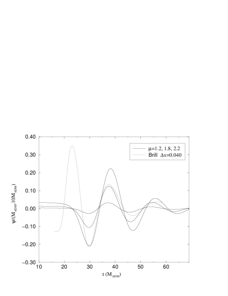
FIG. 3.: We compare the $l$=2,$m$=0 extracted waveform for the head-on collision of BHs obtained by [10] of the $\mu=1.2,1.8,2.2$ Misner data (solid lines, increasing amplitude) to that of the $a=6$ collapsing BW (dotted and dashed lines).

In Fig. 4b we show the {$l$=2,$m$=0} waveform of this 3D case, compared to the previous axisymmetric case. The $c=0.2$ waveform has a longer wave length at late times, consistent with the fact that a larger mass BH is formed in the 3D case. Figs. 4c and 4d show the same comparison for the {$l$=4,$m$=0} and {$l$=2,$m$=2} modes respectively. Notice that while the first two modes are of similar amplitude for both runs, the 3D {$l$=2,$m$=2} mode is completely different; as a non-axisymmetric contribution, it is absent in the axisymmetric run (in fact, it doesn’t quite vanish due to numerical error, but it remains of order $10^{-6}$). We also show a fit to the corresponding QNM’s of a BH of mass 1.0. The fit was performed in the time interval $(10,36)$, and is noticeably worse if the fit is attempted to earlier times, again showing that the lowest QNM’s dominate at around $10$. The early parts of the waveforms $t<10$ reflect the details of the initial data and BH formation process. This is especially clear in the {$l$=2,$m$=2} mode, which seems to provide the most information about the initial data and the 3D BH formation process. At present no 3D BH formation simulation from other scenarios (e.g., true spiraling BH coalescence) are available for comparison, as in the axisymmetric case, but such simulations may actually be available soon [30]. It will be interesting to compare such studies with 3D wave collapses, such as that presented here.

In conclusion, we demonstrated numerical evolutions of 3D, strongly non-linear gravitational waves, and studied gravitational collapse of axisymmetric and non-axisymmetric gravitational waves. We compared the wave collapse to the head-on collision of two black holes. The research opens the door to many investigations.

Acknowledgments. This work was supported by AEI, NCSA, NSF PHY 9600507, NSF MCA93S025 and NASA NCCS5-153. We thank many colleagues at the AEI, Washington University, Univeristat de les Illes Balears, and NCSA for the co-development of the Cactus code, and especially D. Holz for important discussions. Calculations were performed at AEI, NCSA, SDSC, RZG-Garching and ZIB in Berlin.

FIG. 4.: a) The solid (dotted) line is the AH for the full 3D data set $(6,0.2,1)$ ($(6,0,0)$) at $t$=10 on the $x$-$z$ plane. b) The {$l$=2,$m$=0} waveform for the 3D $(6,0.2,1)$ case at $r=4$ (solid line) is compared to axisymmetric $(6,0,0)$ case (dotted line). The dashed line shows the fit of the 3D case to the corresponding mode for a BH of mass 1.0. c) Same comparison for the {$l$=4,$m$=0} waveform. d) Same comparison for the non-axisymmetric {$l$=2,$m$=2} waveform.

REFERENCES

- [1] J. A. Wheeler, Phys. Rev. 97, 511 (1955).
- [2] D. Brill and J. Hartle, Phys. Rev. 135, B271 (1964).
- [3] U. Yurtsever, Phys. Rev. D 38, 1731 (1988).
- [4] A. Abrahams and C. Evans, Phys. Rev. D 46, R4117 (1992).
- [5] A. Abrahams and C. Evans, Phys. Rev. Lett. 70, 2980 (1993).
- [6] C. Gundlach, (1998), gr-qc/9710066.
- [7] M. Shibata and T. Nakamura, Phys. Rev. D 52, 5428 (1995).
- [8] P. Anninos et al., Phys. Rev. D 54, 6544 (1996).
- [9] P. Anninos et al., Phys. Rev. D 56, 842 (1997).
- [10] P. Anninos et al., Phys. Rev. D 52, 2044 (1995).
- [11] C. Bona, J. Massó, E. Seidel, and P. Walker, (1998), gr-qc/9804065. Submitted to Physical Review D.
- [12] M. Alcubierre et al., (1998), in preparation.
- [13] E. Seidel and W.-M. Suen, J. Comp. Appl. Math. (1999), in press.
- [14] G. Allen, K. Camarda, and E. Seidel, (1998), gr-qc/9806036. Submitted to Phys. Rev. D.
- [15] G. Allen, T. Goodale, and E. Seidel, in 7th Symposium on the Frontiers of Massively Parallel Computation-Frontiers 99 (IEEE, New York, 1999).
- [16] D. S. Brill, Ann. Phys. 7, 466 (1959).
- [17] K. Eppley, Phys. Rev. D 16, 1609 (1977).
- [18] K. Eppley, in Sources of Gravitational Radiation, edited by L. Smarr (Cambridge University Press, Cambridge, England, 1979), p. 275.
- [19] D. Holz, W. Miller, M. Wakano, and J. Wheeler, in Directions in General Relativity: Proceedings of the 1993 International Symposium, Maryland; Papers in honor of Dieter Brill, edited by B. Hu and T. Jacobson (Cambridge University Press, Cambridge, England, 1993).
- [20] K. Camarda, Ph.D. thesis, University of Illinois at Urbana-Champaign, Urbana, Illinois, 1998.
- [21] S. Brandt, K. Camarda, and E. Seidel, in Proc. 8th M. Grossmann Meeting, edited by T. Piran (World Scientific, Singapore, 1998), in press.
- [22] M. Alcubierre et al., (1998), gr-qc/9809004.
- [23] T. Baumgarte and S. Shapiro, Physical Review D 59, 024007 (1999).
- [24] J. York, in Sources of Gravitational Radiation, edited by L. Smarr (Cambridge University Press, Cambridge, England, 1979).
- [25] C. Bona and J. Massó, Phys. Rev. Lett. 68, 1097 (1992).
- [26] A. Arbona, C. Bona, J. Massó, and J. Stela, gr-qc/9902053 (1999).
- [27] J. Balakrishna et al., Class. Quant. Grav. 13, L135 (1996).
- [28] A. Abrahams and C. Evans, Phys. Rev. D 37, 318 (1988).
- [29] P. Anninos et al., Phys. Rev. D 52, 4462 (1995).
- [30] B. Brügmann, Int. J. Mod. Phys. D 8, 85 (1999).