Quantum Flux from a Moving Spherical Mirror

Abstract

We calculate the flux from a spherical mirror which is expanding or contracting with nearly uniform acceleration. The flux at an exterior point (which could in principle be a functional of the mirror’s past history) is actually found to be a local function, depending on the first and second time derivatives of acceleration at the retarded time.

I Introduction

Some of the most remarkable predictions of quantum field theory arise from zero point fluctuations of quantum states. One of the best known examples of this is the Unruh effect [1, 2, 3], in which an accelerating detector measures the zero point fluctuations of the inertial (Minkowski) vacuum state and finds they have a thermal spectrum. Another is the Casimir effect [4], in which the walls (or boundaries) of a box experience a net force due to the difference between the zero point fluctuations of the states inside the box and out.

It seems reasonable, then, to expect accelerating boundaries to produce interesting effects, and indeed they do. Following studies of the Casimir effect between moving mirrors in 1+1 dimensions by Moore [5], DeWitt pointed out that the single moving mirror problem would be interesting and could be solved exactly in (1+1)D[6] . Fulling [1] and DeWitt[7] have shown that a uniformly accelerating mirror will indeed alter the quantum state in the vicinity of the mirror. However, a far more interesting result was obtained by Davies and Fulling[8, 9] for a mirror experiencing non-uniform acceleration in (1+1)D. Such a mirror actually emits fluxes of quantum radiation, as though the mirror were knocking zero point quanta out of the vacuum and off to infinity. More precisely, they found that a mirror with 2-velocity $u^{\mu}=dx^{\mu}/d\tau$ ($u\cdot u=-1$) and acceleration $a^{\mu}$ emits a flux

$$\frac{dE}{d\tau}=-\langle T_{\mu\nu}\rangle u^{\mu}n^{\nu}=-\frac{\hbar}{12\pi}\frac{d}{d\tau}~{}(a\cdot n),$$ (1)

in the direction of a unit spatial vector $n^{\nu}$ orthogonal to $u^{\mu}$. This holds for either choice (“left” or “right”) of $n^{\mu}$. Thus, a mirror whose acceleration is increasing (algebraically) toward the right will emit a stream of negative energy to the right and a numerically equal positive stream to the left.

The implications of this result are intriguing. Davies[10] and Ford[11] first raised the possibility that the negative-energy flux from a moving mirror could be used to cool a hot body and thus violate the second law of thermodynamics in a quantum context, and this paradox was further discussed by Deutsch, Ottewill and Sciama[12]. Limitations on the extent of such violations in flat spacetime (“quantum interest”) have been formulated by Ford and Roman[13] and others ([14], [15], etc.).

More recently, Anderson[16] has used this result in the context of the Geroch gedankenexperiment[17]. In this experiment, a box with mirrored walls is filled with radiation and lowered adiabatically toward a black hole. Unruh and Wald[18] have shown that such a box is subject to a buoyancy force and will eventually reach a floating point above the black hole. Anderson has examined this further and shown that the ground state inside the box is the Boulware state, whose energy (which becomes increasingly negative as the box descends) is fed by Davies-Fulling fluxes from the reflecting walls. This accounts for the buoyancy felt by the box.

The volume of literature on moving mirrors is impressive, but it bears noting that all the results mentioned above are obtained in 1+1 dimensions. Indeed, if one includes the result for moving mirrors in curved space-times obtained by Ottewill and Takagi[19] with those reviewed above, the (1+1)D theory of moving mirrors can be considered essentially complete. This is due largely to the conformal properties of quantum field equations in (1+1)D, which allow boundaries, and even space-time itself, to be flattened, thereby enabling one to obtain results for complicated geometries from those for much simpler geometries.

This is not the case in 3+1 dimensions, where only partial results are available. The case of constant acceleration has been solved for both plane[20, 21] and spherical[22] mirror geometries. Ford and Vilenkin[23] have extended the plane mirror result to include non-constant acceleration for the case when the acceleration and its derivatives are small. More recently, Hadasz et al.[24] have considered arbitrary (radial) motion of a spherical mirror, but have restricted their attention to the “S-wave approximation” where only spherically symmetric modes are considered. Because of this restriction, their result can be related to the 1+1 dimensional results of Davies and Fulling[8, 9].

Consideration of quasi-stationary processes (e.g. slow descent of a mirror in a strong gravitational field) requires knowledge of the flux emitted by a mirror whose acceleration is changing slowly, though it may be large. Our objective in this paper is to derive an interesting and relatively simple result of this type in 3+1 dimensions. The central tool is the use of a Green’s function perturbation technique. Evaluating the perturbation is much more manageable if the Green’s functions for the unperturbed problem are available in closed form. This is actually the case for a uniformly accelerated spherical mirror, as shown by Frolov and Serebriany[22]. The mirror’s history is then a three-dimensional pseudo-sphere of radius $b$, say, and the unperturbed problem is just the Minkowski-signature analogue of finding the four-dimensional electrostatic potential of a point charge in the presence of an earthed conducting 3-sphere of radius $b$. This is easily solved by the method of images.

Our objective in this paper is to solve the perturbed Frolov-Serebriany problem, i.e. to examine the effect of small spherically symmetric non-uniformities in the acceleration of a spherical mirror.

It is well to stress at the outset that the solution for a plane mirror cannot be derived from ours by a straightforward limiting process. The single parameter $b$, whose reciprocal gives the unperturbed acceleration, also gives the minimum radius attained by the mirror as seen from its center. Thus, the plane limit $b\rightarrow\infty$ is inseparable from small acceleration. (There are reasons to expect the planar case to be considerably more complicated. Formally, the Wightman Green’s function is now an infinite sum of McDonald (Bessel) functions. Geometrically, any light ray reflected non-orthogonally of a uniformly accelerated plane mirror will re-encounter the mirror an infinite number of times; in the spherical case there is just one encounter.)

Also, we concern ourselves only with calculating the outward flux, which we expect to be the most interesting stress-energy component. In fact, it turns out to be somewhat more interesting than one might expect. We find that it has a remarkable property; although it could, in principle, depend on the entire retarded history of the mirror, to first order in the mirror perturbation it depends only the behavior of the mirror at the most recent retarded time, i.e. it is local.

This article is organized as follows: in Section II we review the Frolov-Serebriany result for a mirror expanding with uniform acceleration. In Section III we present our Green’s function perturbation scheme, and in Section IV we use it to evaluate the corrections to the Frolov-Serebriany Green’s function, with some of the more cumbersome details relegated to Appendix A. Section V is concerned with calculating the quantum flux from these perturbations, with details again left to Appendices (B and C). Finally, in Section VI we offer some concluding remarks.

II Uniformly accelerating spherical mirror

In the case where the mirror’s acceleration is uniform, the Green’s functions for the massless fields can be obtained in simple closed form by the method of images, as noted by Frolov and Serebriany[22]. In this Section we shall briefly review these results.

Consider first the static potential due to a point charge $q^{\prime}$ in Euclidean 4-space at a distance $R^{\prime}$ from the center of an earthed conducting 3-sphere of radius $b$. The Dirichlet boundary condition can be reproduced by introducing a co-radial image charge $q^{\prime\prime}=-(b/R^{\prime})^{2}q^{\prime}$ at radius $R^{\prime\prime}=b^{2}/R^{\prime}$.

In the Lorentzian analogue of this problem, we are concerned with Green’s functions for the wave equation $\Box\varphi=0$ in Minkowski space-time, with Dirichlet boundary conditions on the pseudo-sphere (i.e. the time-like hyperboloid of one sheet) $R=b$, where now

$$R^{2}\equiv\eta_{\mu\nu}x^{\mu}x^{\nu}=x^{2}+y^{2}+z^{2}-t^{2}=\rho^{2}+z^{2}-t^{2},$$ (2)

in a self-evident notation.

The pseudo-sphere $R=b$ represents the history of a spherical mirror of radius $b$ (constant as measured in its instantaneous rest frame), whose center is fixed at the spatial origin $x=y=z=0$ and which moves with uniform acceleration $a=b^{-1}$.

The image construction gives for the retarded Green’s function $G_{ret}(x,x^{\prime})$, satisfying

$$\Box G_{ret}(x,x^{\prime})=-\delta^{4}(x,x^{\prime}),$$ (3)

the expression

$$G_{ret}(x,x^{\prime})=\frac{1}{2\pi}~{}\theta(t-t^{\prime})\left\{\delta[(xx^{\prime})^{2}]-\left(\frac{b}{R^{\prime}}\right)^{2}\delta[(xx^{\prime\prime})^{2}]\right\}.$$ (4)

Here $\theta$ is the unit step (Heaviside) function, $\delta$ is the Dirac distribution, $(xx^{\prime})^{2}$ is the squared Minkowski interval

$$(xx^{\prime})^{2}\equiv\eta_{\mu\nu}(x^{\mu}-{x^{\prime}}^{\mu})(x^{\nu}-{x^{\prime}}^{\nu}),$$ (5)

and the image source is located at

$${x^{\prime\prime}}^{\mu}=\left(\frac{b}{R^{\prime}}\right)^{2}{x^{\prime}}^{\mu}.$$ (6)

Similarly, the Wightman function

$$W(x,x^{\prime})=\langle 0|\varphi(x)\varphi(x^{\prime})|0\rangle$$ (7)

for a massless scalar field takes the form

$$W(x,x^{\prime})=\frac{1}{4\pi^{2}}\left\{\frac{1}{(xx^{\prime})^{2}+i(t-t^{\prime})\epsilon}-\left(\frac{b}{R^{\prime}}\right)^{2}\frac{1}{(xx^{\prime\prime})^{2}+i(t-t^{\prime\prime})\epsilon}\right\},$$ (8)

with $\epsilon\rightarrow+0$.

III Nearly uniform acceleration: perturbing the boundary

The corresponding Green’s functions for a spherical mirror whose acceleration is slightly non-uniform can be derived from the preceding results by superposing the effect of a small perturbation on the history of the mirror, i.e., the time-like 3-space $\Sigma$ on which Dirichlet boundary conditions are imposed.

Consider generally the problem of solving

$$\Box\Phi=0,\hskip 28.45274pt\Phi=0~{}~{}\mbox{on}~{}~{}\Sigma.$$ (9)

Suppose that $\Sigma$ is a small perturbation of a simpler time-like 3-space $\Sigma_{0}$, obtained by displacing $\Sigma_{0}$ a distance $\delta n(x)$ along its outward normal $n$, and that we know the solution $\Phi_{0}$ of the problem

$$\Box\Phi_{0}=0,\hskip 28.45274pt\Phi=0~{}~{}\mbox{on}~{}~{}\Sigma_{0},$$ (10)

with the same initial boundary conditions.

Then (9) can be reformulated as a problem with boundary conditions specified on the unperturbed boundary $\Sigma_{0}$:

$$\Box\Phi=0,\hskip 28.45274pt\Phi=-\frac{\partial\Phi_{0}}{\partial n}~{}\delta n(x)~{}~{}\mbox{ on }~{}~{}\Sigma_{0}.$$ (11)

The causal solution for the perturbation $\delta\Phi\equiv\Phi-\Phi_{0}$ follows from Green’s identity:

$$\delta\Phi(x^{\prime})=\int_{\Sigma_{0}}d\Sigma~{}\frac{\partial G_{ret}(x^{\prime},x)}{\partial n}~{}\delta n(x)~{}\frac{\partial}{\partial n}\Phi_{0}(x),$$ (12)

where $G_{ret}$ is the retarded Green’s function for the unperturbed boundary value problem (10) and $x$ is in $\Sigma_{0}$. Equation (12) defines a linear operation applied to $\Phi_{0}$, which we shall write for brevity as

$$\delta\Phi(x^{\prime})=L_{\delta n}(x^{\prime})~{}\Phi_{0}(\cdot).$$ (13)

To obtain the effect of the perturbation on the Wightman function (7), we note that it can be written as a mode sum

$$W(x,x^{\prime})=\int\frac{d^{3}k}{(2\pi)^{3}}~{}f_{\boldmath{\mbox{${\scriptstyle k}$}}}(x)~{}\overline{f_{\boldmath{\mbox{${\scriptstyle k}$}}}}(x^{\prime}),$$ (14)

where $\{f_{\boldmath{\mbox{${\scriptstyle k}$}}}(x)\}$ is a complete set of initially positive frequency solutions of (9) and the bar denotes complex conjugation. Applying (13) to each mode separately and summing the results yields

$$\delta W(x,x^{\prime})=L_{\delta n}(x)W_{0}(\cdot,x^{\prime})+L_{\delta n}(x^{\prime})W_{0}(x,\cdot),$$ (15)

where $W_{0}$ denotes the unperturbed Wightman function given by (8).

IV Wightman function for nearly uniform acceleration

Evaluation of the expression (15) for $\delta W$ in the case where the mirror’s acceleration departs slightly from uniformity is somewhat lengthy but straightforward. Here, we outline the results of this calculation reserving the technical details for Appendix A.

It will be assumed that the mirror remains spherical as viewed by an observer at its center $x=y=z=0$. Then its history is

$$R=b(1+f(t)),\hskip 28.45274pt|f(t)|\ll 1$$ (16)

in terms of this observer’s time $t$, where $f(t)$ is arbitrary but small. The corresponding advanced and retarded times are written

$$v=t+r,\hskip 28.45274ptu=t-r,\hskip 28.45274ptr=\sqrt{x^{2}+y^{2}+z^{2}}.$$ (17)

The radial energy flux measured by a stationary observer outside the mirror is

$$F=T_{uu}-T_{vv}.$$ (18)

Each of these terms can be dealt with by a similar procedure. Let us consider $T_{uu}$; it is evident from (7) that its expectation value at an event $p_{1}$ outside the mirror is

$$\langle T_{uu}(p_{1})\rangle=\left[\partial_{u_{1}}\partial_{u_{2}}W(p_{1},p_{2})\right]_{p_{2}=p_{1}}$$ (19)

for a minimally coupled massless scalar field, and a similar but more complicated expression for conformal coupling (see (27) below). Note that regularization and symmetrization are not needed to evaluate this component of the stress-energy.

We can now present the results for $\delta W$. The spherical symmetry of (16) allows us to take both $p_{1}$ and $p_{2}$ in the $z-t$ plane ($x=y=0$). Calculation shows (see Appendix A) that the first term of (15) contributes

$$\frac{8\pi^{2}\zeta^{2}}{(R_{1}^{2}-b^{2})(R_{2}^{2}-b^{2})}L_{\delta n}(p_{1})W(\cdot,p_{2})=\frac{z_{1}z_{2}}{\zeta}\int_{-\infty}^{t_{1}^{*}}dt\frac{f(t)}{(t-t_{0})^{3}}-\frac{z_{1}z_{1}^{*}}{(R_{1}^{2}-b^{2})(t_{1}^{*}-t_{0})^{2}}$$ (20)

where $\zeta$ and $t_{0}$ are defined by

$$\zeta=z_{1}t_{2}-z_{2}t_{1},~{}~{}~{}~{}~{}\zeta t_{0}=\frac{1}{2}(z_{1}-z_{2})(z_{1}z_{2}-b^{2})+(z_{1}t_{2}^{2}-z_{2}t_{1}^{2}),$$ (21)

and $p_{i}^{*}$ (with coordinates $x_{i}^{*},t_{i}^{*}$) is the event nearest to $p_{i}$ ($i=1,2$) at which the past light-cone of $p_{i}$ intersects the (unperturbed) mirror (see Fig. 1).

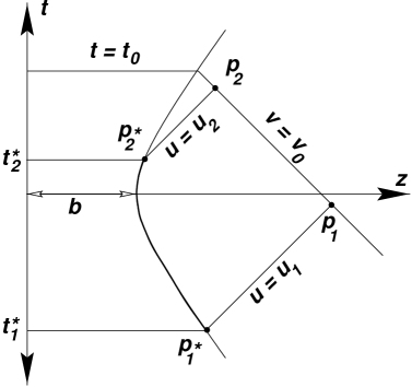
FIG. 1.: The $z-t$ plane. The mirror profile is the hyperbola. $p_{1}$ and $p_{2}$ are the two events at which the Wightman function is to be evaluated and $v_{0}$ is their common advanced time. $p_{1}^{*}$ and $p_{2}^{*}$ are the intersections of their past light-cones with the mirror in the $z-t$ plane.

The contribution of the second term in (15) is obtained by interchanging $p_{1}$ and $p_{2}$ in (20). Because $\zeta$ is an odd function of $p_{1},~{}p_{2}$ ($t_{0}$ is even), the term involving the integral changes sign. Thus, the sum of the two contributions,

$$-\frac{8\pi^{2}\zeta^{2}}{(R_{1}^{2}-b^{2})(R_{2}^{2}-b^{2})}\delta W(p_{1},p_{2})=\frac{z_{1}z_{2}}{\zeta}\int_{t_{1}^{*}}^{t_{2}^{*}}dt\frac{f(t)}{(t-t_{0})^{3}}+\sum_{i=1}^{2}\frac{z_{i}z_{i}^{*}}{(R_{i}^{2}-b^{2})(t_{i}^{*}-t_{0})^{2}}f(t_{i}^{*}),$$ (22)

depends only on the mirror’s history between the retarded times $t_{1}^{*}$ and $t_{2}^{*}$. Particle and anti-particle modes interfere destructively in the case of a spherical mirror to eliminate the effects of the past history and produce (when we take the coincidence limit $p_{2}\rightarrow p_{1}$) a purely local expression for the stress-energy.

To perform the partial derivatives $\partial_{u_{1}}$ and $\partial_{u_{2}}$ in the expression (19) for  $T_{uu}$, we require mutual independence of the $u$-coordinates of the events $p_{1}$ and $p_{2}$. But these are the only coordinates which need be independent. To evaluate $T_{uu}$, it suffices to consider $\delta W(p_{1},p_{2})$ in a partial pre-coincidence limit $v_{1}=v_{2}$, as in Fig. 1.

These remarks in principle apply, mutatis mutandis, also to the evaluation of  $T_{vv}$, but there is a complication. In the pre-coincidence limit $u_{2}\rightarrow u_{1}$, the points $p_{1}^{*}$ and $p_{2}^{*}$ tend to coincidence with each other and with the point on the mirror having coordinate $t_{0}$, so that the integrand in (22) becomes infinite while the interval of integration shrinks to zero. The evaluation of $T_{vv}$ is discussed further in Appendix C. Here, we merely note that $T_{vv}$ makes no radiative contribution (proportional to $r^{-2}$) to the flux (19). This follows at once from the identity

$$\partial_{u}\left(r^{2}\partial_{u}\left(r^{2}T_{vv}\right)\right)=\partial_{v}\left(r^{2}\partial_{v}\left(r^{2}T_{uu}\right)\right),$$ (23)

which is a consequence of the conservation of $T_{\mu\nu}$ and the vanishing of the trace $T^{\alpha}_{\alpha}$ for a conformal scalar field in flat space. In (23), the derivative $\partial_{v}$ increases the fall-off with distance, but this does not hold for $\partial_{u}$, which can operate on the retarded displacement $f(u)$ in (16). Thus, $T_{vv}$ falls off more strongly than $T_{uu}$. The detailed calculation (Appendix C) shows that $T_{vv}\sim r^{-6}$ as $r\rightarrow\infty$.

V Flux from a non-uniformly accelerating mirror

The expectation value of the stress-energy is derivable from the partial derivatives of the Wightman function $W(x,x^{\prime})=W_{0}+\delta W$ in the coincidence limit, with the unperturbed part $W_{0}$ given by (8) and the perturbation $\delta W$ by (22). The unperturbed part becomes singular in the limit $x^{\prime}\rightarrow x$, but is easily regularized by subtracting the value of $W_{0}$ in free space without the mirror, i.e., the first term of (8), leaving the second (image) term as the sole contribution to $(W_{0})_{reg}$. The perturbation $\delta W$ is regular in the coincidence limit.

For a massless scalar field, two different stress tensors are commonly considered: (a) the minimal stress-energy, given classically by

$$\left(T_{\mu\nu}\right)_{min}=\varphi_{,\mu}\varphi_{,\nu}-\frac{1}{2}g_{\mu\nu}(\nabla\varphi)^{2}$$ (24)

and quantum mechanically by

$$\langle T_{\mu\nu}(x)\rangle_{min}=\left[(\partial_{\mu}\partial_{\nu^{\prime}}-\frac{1}{2}g_{\mu\nu}~{}\partial^{\alpha}\partial_{\alpha^{\prime}})W_{reg}(x,x^{\prime})\right]_{sym~{};~{}x^{\prime}=x},$$ (25)

in which “sym” indicates symmetrization in (x,x’) and in the partial derivatives; (b) the conformal (trace-free) stress-energy, defined classically by

$$\left(T_{\mu\nu}\right)_{\mathit{c}onf}=\frac{2}{3}\varphi_{,\mu}\varphi_{,\nu}-\frac{1}{3}\varphi\varphi_{,\mu\nu}-\frac{1}{6}g_{\mu\nu}(\nabla\varphi)^{2}$$ (26)

and quantum mechanically by

$$\langle T_{\mu\nu}(x)\rangle_{\mathit{c}onf}=\frac{1}{3}\left[(2\partial_{\mu}\partial_{\nu^{\prime}}--\partial_{\mu^{\prime}}\partial_{\nu^{\prime}}-\frac{1}{2}g_{\mu\nu}~{}\partial^{\alpha}\partial_{\alpha^{\prime}})W_{reg}(x,x^{\prime})\right]_{sym~{};~{}x^{\prime}=x},$$ (27)

We begin by reviewing the Frolov-Serebriany[22] results for uniform acceleration. Differentiating the regularized form of (8), we easily find

$$\langle T^{(0)}_{\mu\nu}(x)\rangle_{min} = -\frac{b^{2}}{\pi^{2}(R^{2}-b^{2})^{4}}\left(x^{\mu}x^{\nu}-\frac{1}{2}g^{\mu\nu}R^{2}\right),$$ (28)

$$\langle T^{(0)}_{\mu\nu}(x)\rangle_{\mathit{c}onf} = 0.$$ (29)

This last result is quite remarkable, because the conformal stress is not likely to vanish for a spherical mirror at rest (it certainly does not for electromagnetic fields [25, 10, 26]). It appears that the effects of uniform acceleration exactly cancel the static Casimir stresses.

The effects of non-uniform acceleration are more complicated. We shall simply quote the result for the conformal radial out-flux $\langle T_{uu}\rangle_{\mathit{c}onf}$ at a point $(r,t)$ outside the mirror, leaving to Appendix B an outline of the derivation:

$$\langle T_{uu}(t,r)\rangle_{\mathit{c}onf}=-\frac{1}{1440\pi^{2}}\frac{1}{rv}\left\{\frac{q}{m^{3}n}\frac{d^{2}\alpha}{d\chi^{2}}-\frac{4}{m^{3}n^{2}r}(npr-q^{2})\frac{d\alpha}{d\chi}+\frac{2s^{2}}{mn^{3}r^{2}}\left[q(\alpha+f)+p\frac{df}{d\chi}\right]\right\}.$$ (30)

The notation is as follows: the advanced and retarded times, $v$ and $u$ are defined as in (17), and we write

$$m = -\frac{u}{2},~{}~{}~{}n~{}=~{}\frac{1}{2v}(R^{2}-b^{2})~{}=~{}-\frac{1}{2}(u+b^{2}/v),$$ (31)

$$p = \frac{1}{8}(u^{2}-b^{2}),~{}~{}~{}q~{}=~{}\frac{1}{8}(u^{2}+b^{2}),~{}~{}~{}s~{}=~{}-\frac{1}{2}(v+b^{2}/v);$$ (32)

$\chi$ is the pseudo-angle along the (unperturbed) mirror trajectory (i.e., $\tau=b\chi$ is the mirror’s proper time). Equation (16), giving the trajectory of the perturbed mirror, is now written $R=b(1+f(\chi))$, and

$$\alpha=f^{\prime\prime}(\chi)-f(\chi)$$ (33)

is a measure of the non-uniformity of the acceleration $A$, which is given by

$$A=(1+\alpha)/b.$$ (34)

In (30), $\chi$ refers to the pseudo-angle at the point $p^{*}$, which is the nearest retarded point to (r,t), as in Fig. 2. The corresponding expression for the canonical flux is too long to reproduce here, and is also deferred to Appendix B.

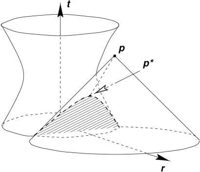
FIG. 2.: Intersection of the history of a uniformly accelerating sphere (hyperboloidal cylinder) and the past null cone of an exterior point $p$. The intersection (which lies entirely within the shaded plane) is represented by the bold curve. The nearest retarded point to $p$ on the mirror’s worldsheet, $p^{*}$, is the only point whose perturbation contributes to the flux at $p$. This figure has been dimensionally reduced; each point represents a circle.

The limit $b\rightarrow\infty$ corresponds to a slowly accelerating, nearly plane mirror. This was the case studied by Ford and Vilenkin[23]. It is straightforward to show that in this limit our result (30) for the conformal flux (and also our result for the canonical flux) reduces to the expressions they give.

To obtain a more intuitive grasp of the physical meaning of the complex expression (30), we can evaluate the flux $F$ radiated at retarded time $u=-b$   -   i.e. when the mirror is near its minimum radius $r_{M}\approx b$   -   as measured by a stationary observer at radius $r\gg b$ and the same retarded time. Using (18), taking the appropriate limit of (30), and noting that $T_{vv}$ does not contribute to the flux to leading order (as discussed at the end of Section IV) we find

$$F=-\frac{\hbar}{720\pi^{2}}\left(\frac{R_{0}}{r}\right)^{2}\left\{A\frac{d^{2}A}{d\tau^{2}}+2A^{3}\left(A-\frac{1}{R_{0}}\right)\right\},$$ (35)

where $R_{0}=b(1+f(0))$ is the proper radius of the mirror at the time of emission $\chi=0$, and we have restored Planck’s constant to display the correct dimensionality. We recall that this perturbative result is correct to linear order in deviations from uniform acceleration $(A-1/R)$, $dA/d\tau$, $d^{2}A/d\tau^{2}$, but the acceleration $A$ itself is arbitrary.

VI Concluding Remarks

Our chief interest in this paper has been in the quantum flux radiated by the mirror and we have explicitly computed only those components of the stress-energy tensor from which it arises. However, the remaining components can be derived straightforwardly (though with some labour) from our expression (22) with the methods of Appendix B. It would be useful to have these to round out the picture.

The relevant Green’s functions for an unperturbed, uniformly accelerating spherical mirror have a simple closed form, and this has enormously simplified our perturbative calculation. This simplification is bought at a price: we are limited to spherical mirrors whose acceleration $A$ and proper radius $R$ are nearly reciprocals. We cannot decouple the plane limit $R\rightarrow\infty$ from the limit of small acceleration, and cannot disentangle curvature (Casimir) effects from the effects of acceleration.

It is evident that much remains to be done before we can claim anything approaching a comprehensive understanding of the quantum dynamics of three-dimensional mirrors.

A Evaluation of the integral (3.7) for $\delta W$

To verify (22), one needs to evaluate $L_{\delta n}(p_{1})~{}W_{0}(\cdot,p_{2})$, where the integral operator $L_{\delta n}$ is defined by (13) and $W_{0}$ by (8). Because of the spherical symmetry of the mirror, there is no loss of generality in taking $p_{1}$ to be in the $z-t$ plane. Then the integration over the azimuthal cylindrical coordinate $\phi$ is trivial.

The problem is essentially solved by the following lemma. Let $F(p)=F(\rho,z,t)$ be any axisymmetric function. Then we have the identity

$$\int_{\Sigma_{0}}F(p)~{}\frac{\partial}{\partial n}G_{ret}(p_{1},p)~{}d\Sigma=-\mbox{sgn}(R^{2}-b^{2})~{}\frac{z_{1}^{*}}{z_{1}}~{}F(p_{1}^{*})$$ (A1)

$$~{}~{}~{}~{}~{}~{}~{}~{}~{}~{}+\frac{1}{2}~{}\mbox{sgn}(z_{1})~{}\frac{R_{1}^{2}-b^{2}}{z_{1}^{2}}~{}\int_{-\infty}^{t_{1}^{*}}dt~{}\left[\frac{\partial}{\partial z}~{}F(\rho=\sqrt{b^{2}+t^{2}-z^{2}},z,t)\right]_{z=Z_{1}(t)}$$ (A2)

where $p_{1}^{*}$ is defined as in Section IV and the linear function $z=Z_{1}(t)$ is the solution of $\xi(p_{1},p)=0$ where

$$\xi(p_{1},p)\equiv t_{1}t-z_{1}z+\frac{1}{2}(R_{1}^{2}+b^{2}).$$ (A3)

Geometrically, $z=Z_{1}(t)$ represents the line in the $z-t$ plane through $p_{1}^{*}$ and orthogonal to the radius vector joining $p_{1}$ to the origin $z=t=0$.

To prove (A2), let us note that the presence of $G_{ret}$ will effectively confine the integration to a 2-space ${\cal S}$, formed by the intersection of the unperturbed mirror’s history

$$\Sigma_{0}~{}~{}:~{}~{}\sigma(0,p)=\frac{1}{2}b^{2}$$ (A4)

with the past light-cone of $p_{1}$, given by

$$\sigma(p_{1},p)=0,$$ (A5)

where $\sigma(p_{1},p_{2})=\frac{1}{2}(p_{1}~{}p_{2})^{2}$ is the usual geodesic biscalar (c.f. (5) and see Fig. 2). Taking the difference between (A4) and (A5), we see that ${\cal S}$ can equivalently be regarded as the intersection of the mirror $\Sigma_{0}$ with the 3-plane $\xi(p_{1},p)=0$, where

$$\xi(p_{1},p)=\sigma(p_{1},p)-\sigma(0,p)+\frac{1}{2}b^{2}$$ (A6)

is the same as (A3).

$G_{ret}$ in the integral (A2) is a (distributional) function of $\sigma(p_{1},p)$ and $\sigma(p_{1},\tilde{p})$ (see (4)), where $\tilde{p}$ is the image point of $p$. To obtain its normal derivative on the mirror $R=b$, it is convenient to introduce four dimensional polar coordinates for $p$,

$$\rho=R\cosh\chi\sin\theta,~{}~{}~{}~{}~{}z=R\cosh\chi\cos\theta,~{}~{}~{}~{}~{}t=R\sinh\chi,$$ (A7)

so that the normal derivative (“outward” from $\Sigma_{0}$ as viewed from the point $p$ outside $\Sigma_{0}$) corresponds to $-\partial/\partial R$. We easily find

$$2~{}\sigma(p_{1},p) = R^{2}+2R(t_{1}\sinh\chi-z_{1}\cosh\chi\cos\theta)+R_{1}^{2},$$ (A8)

$$\left.\frac{\partial}{\partial R}\sigma(p_{1},p)\right|_{R=b} = \frac{1}{b}\left[\xi(p_{1},p)-\frac{1}{2}(R_{1}^{2}-b^{2})\right].$$ (A9)

A similar calculation for the image contribution yields values for $2\sigma(p_{1},\tilde{p})$ and $\frac{\partial}{\partial R}\sigma(p_{1},\tilde{p})$ numerically equal to (A8) and (A9) on the mirror, but for the normal derivative the sign is opposite.

The element of 3-area $d\Sigma$ on the mirror

$$\Sigma_{0}~{}~{}:~{}~{}\rho=\sqrt{b^{2}+t^{2}-z^{2}},$$ (A10)

employing $(t,z,\phi)$ as intrinsic coordinates, is $d\Sigma=b~{}d\phi~{}dz~{}dt$. Hence the integral of an axisymmetric function $H(\rho,z,t)$ takes the explicit form

$$\int_{\Sigma_{0}}d\Sigma~{}H(\rho,z,t)=2\pi b\int_{-\infty}^{\infty}\int_{-\infty}^{\infty}dt~{}dz~{}\theta(b^{2}+t^{2}-z^{2})~{}H(\rho=\sqrt{b^{2}+t^{2}-z^{2}},z,t)$$ (A11)

in which the step function $\theta$ takes into account that, for fixed $t$, the range of $z$ over $\Sigma_{0}$ is restricted by (A10).

The distributional factors $\delta^{\prime}[2\sigma(p_{1},p)]$ and $\delta[2\sigma(p_{1},p)]$, which arise from $\partial G_{ret}(p_{1},p)/\partial n$ in the integral over $\Sigma_{0}$, are handled as follows. For points $p$ restricted to $\Sigma_{0}$, (A4) and (A6) show that $\sigma(p_{1},p)=\xi(p_{1},p)$, given explicitly in (A3) in terms of the intrinsic coordinates $(t,z,\phi)$ of $\Sigma_{0}$. Taking the partial derivatives with respect to $z$ tangentially along $\Sigma_{0}$ (i.e., holding $\phi$ and $t$ fixed in $\xi$), we immediately find

$$\frac{\partial}{\partial z}\delta[2\sigma(p_{1},p)]=-2zz_{1}\delta^{\prime}[2\sigma(p_{1},p)].$$ (A12)

Thus, $\delta^{\prime}$ can be eliminated in favor of the tangential derivative $\partial\delta/\partial z$, which can be converted through integration by parts in (A11) to

$$\delta[2\sigma(p_{1},p)]=\delta[2\xi(p_{1},p)]=\frac{1}{2~{}|z_{1}|}~{}\delta(z-Z_{1}(t)),$$ (A13)

by virtue of (A3).

Putting all this together leads straightforwardly to the quoted result (A2).

B Derivation of (5.7) for the conformal flux

We briefly outline how the formula (30) for $\langle T_{uu}\rangle_{conf}$ is derived from (22) via (27).

$\delta W$ involves the integral

$$z_{1}~{}z_{2}~{}\int_{t_{1}^{*}}^{t_{2}^{*}}\frac{f(t^{*})}{(t^{*}-t_{0})^{3}}dt^{*}.$$ (B1)

Because of the prefactor $z_{1}z_{2}$, it is convenient to change the variable of integration from $t$ (the coordinate of a point $p$ on the profile of $\Sigma_{0}$ in the $z-t$ plane) to $z$ (the coordinate of a point $p$ on the line $v=v_{0}$ joining $p_{1}$ and $p_{2}$, and having the same retarded time, $u=u^{*}$). Since $t^{*}=\frac{1}{2}(u^{*}+v^{*})=\frac{1}{2}(u-b^{2}/u)$ for a point $p^{*}$ on $\Sigma_{0}$ and $z=\frac{1}{2}(v_{0}-u)$, the formal transformation is

$$t^{*}-t_{0}=-\frac{z}{uv_{0}}(b^{2}+uv_{0}),~{}~{}~{}~{}~{}t_{0}=\frac{1}{2v_{0}}(v_{0}^{2}-b^{2}).$$ (B2)

We thus find

$$\frac{1}{2}f(t^{*})\frac{dt^{*}}{(t^{*}-t_{0})^{3}}=A(z)dz,~{}~{}~{}~{}~{}A(z)=\frac{mq}{[z(z+s)]^{3}}~{}f(t^{*}),$$ (B3)

where $m$, $q$ and $s$ are defined in (32), and here $v=v_{0}$.

Writing, for any function $F(z)$,

$$\bar{F}=\frac{1}{2}\left\{\rule[2.25555pt]{0.0pt}{6.76666pt}F(z_{1})+F(z_{2})\right\},~{}~{}~{}~{}~{}\Delta F=F(z_{2})-F(z_{1}),$$ (B4)

the expression (22) for $\delta W$ now reduces to

$$\frac{\pi^{2}v_{0}(\Delta z)^{2}}{(z_{1}+s)(z_{2}+s)}\delta W(p_{1},p_{2})=\frac{z_{1}z_{2}}{\Delta z}\int_{z_{1}}^{z_{2}}A(z)dz-\overline{z^{2}A(z)}.$$ (B5)

It is now straightforward, though tedious, to carry out the operations in (27). The following general identities are of help in this regard. Define, for an arbitrary $F(z)$,

$$\epsilon=\frac{1}{\Delta z}\int_{z_{1}}^{z_{2}}F(z)dz-\bar{F}.$$ (B6)

Then

$$\frac{\epsilon}{(\Delta z)^{2}} = -\frac{1}{12}~{}\overline{F^{\prime\prime}}+\frac{1}{120}~{}(\Delta z)^{2}~{}\overline{F^{(4)}}+\ldots$$ (B7)

$$\frac{\Delta F}{\Delta z} = \overline{F^{\prime}}-\frac{1}{12}~{}(\Delta z)^{2}~{}\overline{F^{\prime\prime\prime}}+\frac{1}{120}~{}(\Delta z)^{4}~{}\overline{F^{(5)}}+\ldots$$ (B8)

where primes and subscripts in parentheses denote derivatives with respect to $z$. If

$$J=\frac{1}{(\Delta z)^{2}}\left\{\frac{z_{1}z_{2}}{\Delta z}\int_{z_{1}}^{z_{2}}F(z)dz-\overline{z^{2}F}\right\}$$ (B9)

then

$$\frac{\partial^{2}J}{\partial z_{1}z_{2}}=-2\frac{\epsilon}{(\Delta z)^{2}}\left(1+\frac{6z_{1}z_{2}}{(\Delta z)^{2}}\right)+\frac{2}{(\Delta z)^{2}}+\left(\frac{\Delta(zF)}{\Delta z}-\bar{F}-\frac{1}{2}\frac{\Delta(z^{2}F^{\prime})}{\Delta z}\right).$$ (B10)

Taking coincidence limits $z_{2}\rightarrow z_{1}$ gives

$$\left[\frac{\partial^{2}J}{\partial z_{1}\partial z_{2}}\right] = -\frac{1}{60}(z^{2}F^{(4)}+10zF^{\prime\prime\prime}+20F^{\prime\prime}),$$ (B11)

$$\left[\rule[2.9514pt]{0.0pt}{8.85422pt}\overline{\frac{\partial J}{\partial z}}\right] = -\frac{1}{24}(z^{2}F^{\prime\prime\prime}+8zF^{\prime\prime}+12F^{\prime}),$$ (B12)

$$\left[J\right] = -\frac{1}{12}(z^{2}F^{\prime\prime}+6(zF)^{\prime}),$$ (B13)

$$\left[\rule[2.9514pt]{0.0pt}{10.388pt}\overline{\frac{\partial^{2}J}{\partial z^{2}}}\right] = \frac{3}{2}\left[\frac{\partial^{2}J}{\partial z_{1}\partial z_{2}}\right].$$ (B14)

A fairly long calculation then leads to the result (30) for the conformal flux. For the canonical flux, we find

$$\delta\langle T_{uu}\rangle_{min}=\frac{1}{240\pi^{2}vr}\left\{\frac{q}{m^{3}n}~{}\frac{d^{2}\alpha}{d\chi^{2}}+a_{1}\frac{d\alpha}{d\chi}+a_{2}~{}\alpha+a_{3}~{}\frac{1}{m}\left(f-\frac{df}{d\chi}\right)+a_{4}~{}mf\right\}$$ (B15)

as the perturbation of the uniform acceleration result (28). Here,

$$a_{1} = \frac{1}{2mn}+\frac{1}{mr}+\frac{r}{m^{3}n^{2}}\left(\frac{7}{2}m^{2}-n^{2}-\frac{5}{2}mn\right),$$ (B16)

$$a_{2} = -\frac{1}{2mn}+\frac{3}{2}\frac{1}{n^{2}}+\frac{3}{2}\frac{1}{nr}+\frac{1}{r^{2}}+\frac{16r}{n^{3}}-\frac{16r}{mn^{2}}-\frac{1}{mr},$$ (B17)

$$a_{3} = -\frac{1}{2n}+\frac{3}{2}\frac{m}{nr}-2\frac{m^{2}}{nr^{2}}-\frac{1}{r}+\frac{m}{r^{2}}+\frac{3}{2}\frac{m}{n^{2}}-\frac{m^{2}}{n^{2}r}$$ (B19)

$$~{}~{}~{}~{}~{}~{}~{}~{}~{}~{}-\frac{2m^{2}}{n^{3}}+\frac{16r(m-n)}{n^{3}}-\frac{45m(m-n)r}{n^{4}},$$

$$a_{4} = \frac{2}{n^{3}}+\frac{1}{n^{2}r}+\frac{2}{nr^{2}}+\frac{60(m-n)r}{n^{5}}.$$ (B20)

C Evaluation of $T_{vv}$

For arbitrary points $p_{1}$ and $p_{2}$ in the $z-t$ plane, the expression (22) for $\delta W$ can be recast in the form

$$-\frac{2\pi^{2}}{\Delta u} (\bar{v}\Delta u-\bar{u}\Delta v)^{3} \delta W(p_{1},p_{2})$$ (C3)

$$=(R_{1}^{2}-b^{2})(R_{2}^{2}-b^{2})\left\{\frac{z_{1}z_{2}}{\Delta z}\int_{z_{1}}^{z_{2}}H(z)dz-\overline{z^{2}H}\right\}$$

$$~{}~{}~{}~{}+\frac{1}{2}\Delta v\left\{(u_{1}u_{2}\bar{v}+b^{2}\bar{u})\Delta(z^{2}H)-(u_{1}u_{2}\Delta v-b^{2}\Delta u)\overline{z^{2}H}\right\},$$

which generalizes (B5) to the case where $\Delta v=v_{2}-v_{1}\neq 0$. The integral of $H(z)$ is to be taken along the straight-line segment joining $p_{1}$ and $p_{2}$, and we have defined

$$H(z)=\frac{u(u^{2}+b^{2})}{[u(t^{*}-t_{0})]^{3}}f(t^{*}).$$ (C4)

The denominator involves a quadratic function of retarded time, having the explicit form

$$u(t^{*}-t_{0})=\frac{1}{2}(u^{2}-cu-b^{2}),$$ (C5)

where

$$c=\frac{(\bar{v}^{2}-b^{2})\Delta u-(\bar{u}^{2}-b^{2})\Delta v-\frac{1}{2}\Delta u\Delta v\Delta z}{\bar{v}\Delta u-\bar{u}\Delta v}.$$ (C6)

By assigning different values to the ratio $\Delta v/\Delta u$ as $\Delta u\rightarrow 0$, we approach the coincidence limit $p_{1}=p_{2}$ in all possible directions in the $z-t$ plane. (This is subject to the restriction that $t_{0}$, given by (21), should be kept outside the interval $(t_{1}^{*},t_{2}^{*})$ to keep the integral of $H$ in (C3) mathematically well defined.) Both of the components $T_{uu}$ and $T_{vv}$ can thus be found from the corresponding directional derivatives.

We calculated $T_{vv}$ with the aid of the computer algebra package MAPLE. Even so, the calculation is not straightforward. The main obstacle is the evaluation of the integral term in (C3). After taking the appropriate $v_{1}$ and $v_{2}$ derivatives of (C3), and then the partial coincidence limit $v_{2}\rightarrow v_{1}$, we express the integrand of the first term in a Laurent series in $(u_{2}-u_{1})$ and $(u-u_{1})$, both to fifth order. The result is expressed in ratios of powers of $(u-u_{1})$ and $(u_{2}-u_{1})$, with coefficients of these ratios being functions of $u_{1}$ and $v_{1}$ alone. The integration is then trivially performed. The first two terms in the integrated Laurent series diverge in the coincidence limit $u_{2}\rightarrow u_{1}$. However, these are exactly cancelled by terms arising from the $v$ derivatives of the second term of (C3). Taking the (trivial) coincidence limit of the remaining terms we find the following expression for $T_{vv}$,

$$T_{vv}=-\frac{1}{45\pi^{2}}\frac{q^{2}}{v^{3}n^{3}r^{3}m}\left(q(\alpha+f)+p\frac{df}{d\chi}\right),$$ (C7)

where our notation is defined in (32). We have verified that the expressions (C7) for $T_{vv}$ and (30) for $T_{uu}$ satisfy the conservation identity (23).

REFERENCES

- [1] S. A. Fulling, Phys. Rev. D7, 2850 (1973).
- [2] P. C. W. Davies, J. Phys. A8, 609 (1975).
- [3] W. G. Unruh, Phys. Rev. D14, 870 (1976).
- [4] H. B. G. Casimir, Proc. Kon. Ned. Akad. Wet. 51, 793 (1948).
- [5] G. T. Moore, J. Math. Phys. (NY) 9, 2679 (1970).
- [6] B. S. DeWitt, in Particles and Fields - 1974, edited by C. E. Carlson (American Institute of Physics, New York, 1974), pp. 660 – 668.
- [7] B. S. DeWitt, Phys. Rep. 19, 295 (1975).
- [8] S. A. Fulling and P. C. W. Davies, Proc. R. Soc. London A348, 393 (1976).
- [9] P. C. W. Davies and S. A. Fulling, Proc. R. Soc. London A356, 237 (1977).
- [10] B. Davies, J. Math. Phys. (NY) 13, 1324 (1972).
- [11] L. H. Ford, Proc. R. Soc. London A364, 227 (1978).
- [12] D. Deutsch, A. C. Ottewill, and D. W. Sciama, Phys. Lett. 119B, 72 (1982).
- [13] L. H. Ford and T. A. Roman, The Quantum Interest Conjecture, gr-qc/9901074.
- [14] E. E. Flanagan, Phys. Rev. D56, 4922 (1997).
- [15] F. Pretorius, Quantum interest for scalar fields in Minkowski spacetime, gr-qc/9903055.
- [16] W. G. Anderson, Phys. Rev. D50, 4786 (1994).
- [17] J. D. Bekenstein, Phys. Rev. D23, 287 (1981).
- [18] W. G. Unruh and R. M. Wald, Phys. Rev. D25, 942 (1982).
- [19] A. C. Ottewill and S. Takagi, Prog. Theor. Phys. 79, 429 (1988).
- [20] P. Candelas and D. Deutsch, Proc. R. Soc. London A354, 79 (1977).
- [21] P. Candelas and D. Deutsch, Proc. R. Soc. London A362, 255 (1978).
- [22] V. P. Frolov and E. M. Serebriany, J. Phys. A12, 2415 (1979).
- [23] L. H. Ford and A. Vilenkin, Phys. Rev. D25, 2569 (1982).
- [24] L. Hadasz, M. Sadzikowski, and P. Wȩgrzyn, Quantum Radiation from Moving Spherical Mirrors, hep-th/9803032, 1998.
- [25] T. H. Boyer, Phys. Rev. 174, 1764 (1968).
- [26] K. A. Milton, L. L. DeRaad, and J. Schwinger, Ann. Phys. (NY) 115, 388 (1978).