Abstract

Although quantum field theory allows local negative energy densities and fluxes, it also places severe restrictions upon the magnitude and extent of the negative energy. The restrictions take the form of quantum inequalities. These inequalities imply that a pulse of negative energy must not only be followed by a compensating pulse of positive energy, but that the temporal separation between the pulses is inversely proportional to their amplitude. In an earlier paper we conjectured that there is a further constraint upon a negative and positive energy delta-function pulse pair. This conjecture (the quantum interest conjecture) states that a positive energy pulse must overcompensate the negative energy pulse by an amount which is a monotonically increasing function of the pulse separation. In the present paper we prove the conjecture for massless quantized scalar fields in two and four-dimensional flat spacetime, and show that it is implied by the quantum inequalities.

1 Introduction

Known forms of classical matter obey the weak energy condition (WEC): $T_{\mu\nu}u^{\mu}u^{\nu}\geq 0$, where $T_{\mu\nu}$ is the stress-energy tensor of matter, and $u^{\mu}$ is an arbitrary timelike vector [1]. By continuity, the condition also holds for all null vectors. Physically, the WEC implies that the energy density seen by any observer must be non-negative. However, the renormalized stress-energy tensors of quantum fields can violate the WEC, as well as all other known pointwise energy conditions [2, 3]. States of quantum fields which involve negative energy densities have even been produced in the laboratory, two examples being the Casimir effect [4, 5, 6, 7] and squeezed states of light [8], although the energy densities have not been directly measured. If there were no constraints on negative energy densities, then it would be possible to use them to produce macroscopic effects. Such effects might include warp drives [9, 10], traversable wormholes [11], time machines [12, 13, 14], and violations of the second law of thermodynamics [15, 16]. The extent to which the laws of physics place restrictions on negative energy density has received much attention during the last few years.

Recent progress has been made on the topic of “quantum inequalities.” These are inequalities which restrict the magnitude and duration of negative energy densities and fluxes [15, 17, 18, 19, 20, 21]. Physically, the inequalities imply that the energy density seen by an observer cannot be arbitrarily negative for an arbitrarily long period of time [22]. The mathematical form of the bound consists of the renormalized expectation value of the energy density or the flux, evaluated in an arbitrary quantum state, and folded into a sampling function. The latter is a peaked function of time with a characteristic width, $t_{0}$, called the sampling time. For a quantized massless, minimally coupled scalar field in four-dimensional Minkowski spacetime, the original bound on the energy density has the form [20, 21]:

$$\hat{\rho}\equiv{{t_{0}}\over\pi}\,\int_{-\infty}^{\infty}\,{{T_{\mu\nu}u^{\mu}u^{\nu}\,dt}\over{t^{2}+{t_{0}}^{2}}}\geq-{3\over{32{\pi}^{2}{t_{0}}^{4}}}\,,$$ (1)

for all sampling times $t_{0}$, where $t$ is the proper time of a geodesic observer. (Throughout this paper we use units in which $\hbar=c=1$.) Equation (1) was derived using the Lorentzian sampling function given by

$$g(t)=\frac{t_{0}}{\pi\,(t^{2}+{t_{0}}^{2})}\,.$$ (2)

Quantum inequalities have now been derived in curved as well as flat spacetimes, in both two and four dimensions [23, 24, 25, 26]. They have also been used to obtain severe constraints on traversable wormhole geometries [27] and warp drives [28, 29]. Quantum inequalities have been derived for massless and massive scalar fields [20, 21, 23, 25, 26], and for the electromagnetic field [21].

Flanagan [30] generalized the original two-dimensional flat spacetime inequalities to those with arbitrary sampling functions and was also able to find the optimal bound. His result is

$${\hat{\rho}}_{min}=-\frac{1}{24\,\pi}\,\int_{-\infty}^{\infty}\,\frac{{g^{\prime}(t)}^{2}}{g(t)}\,dt\,,$$ (3)

where $g(t)$ is an arbitrary sampling function. If the Lorentzian sampling function is substituted into Eq. (3), the resulting bound is a factor of six smaller than the original two-dimensional bound found in Refs. [20, 21].

Fewster and Eveson (FE) [31] have discovered a much simpler method for deriving the quantum inequalities than was given previously. They prove quantum inequalities for massless and massive scalar fields in two and four- dimensional flat spacetimes. Their result for the massless scalar field in four dimensions is given by

$$\hat{\rho}\geq-\frac{1}{16\,{\pi}^{2}}\,\int_{-\infty}^{\infty}\,{\bigl{(}{g^{1/2}}^{\prime\prime}(t)\bigr{)}}^{2}\,dt\,,$$ (4)

where again $g(t)$ is an arbitrary sampling function. When $g(t)$ is chosen to be the Lorentzian sampling function, the resulting bound is $9/64$ of that in Eq. (1).

An extremely useful feature of the results of Flanagan and of FE is the freedom to employ sampling functions with compact support. Some use of this type of sampling function has already been made in Ref. [32]. This freedom will be exploited more fully in the current paper.

In an earlier paper [19], we found evidence to suggest that there may be stronger restrictions on negative energy densities than those proved to date. There we were concerned with the question of whether a $\delta$-function pulse of negative energy injected into an extreme charged black hole could produce an observable violation of cosmic censorship by making the mass temporarily less than the charge. We showed that any initial negative $(-)$ energy pulse had to be accompanied by a subsequent positive $(+)$ energy pulse. (The use of $\delta$-function pulses would seem to provide an efficient means of separating $(-)$ and $(+)$ energy.) Furthermore, we discovered that there existed a quantum inequality-type constraint on the magnitude of the $(-)$ energy pulse and the time separation between the pulses. Similar constraints had also been found for pulses in flat spacetime [17]. This inequality appeared to exclude the possibility of an unambiguously observable violation of cosmic censorship.

During the course of that investigation we discovered that, at least in certain instances, it was not possible to make the pulses exactly compensate one another. It appeared that the $(+)$ pulse had to overcompensate the $(-)$ pulse. Furthermore, it appeared that the amount of overcompensation increased with increasing time separation of the pulses. This behavior suggested to us that a more general principle might be at work. We called this the “quantum interest conjecture”, which states that an energy “loan”, i. e., $(-)$ energy, must always be “repaid”, i. e., by $(+)$ energy, with an “interest” which depends on the magnitude and duration of the loan. In the present paper, we prove that the conjecture is indeed true, at least for $\delta$-function pulses composed of massless scalar fields in Minkowski spacetime.

In Sec. 2, we present a physically transparent example of quantum interest in two dimensions, where the $\delta$-function pulses are generated by a moving mirror. It is shown in Sec. 3 that there exists a general constraint on the maximum pulse separation, which is derived using a quantum inequality with compactly- supported sampling functions. In Sec. 4 we show that quantum interest is required to exist for $\delta$-function pulses in two and four-dimensional flat spacetime, even for arbitrarily small pulse separations. Our conclusions and some remaining open questions are discussed in Sec. 5.

2 A Simple Example: The Moving Mirror

As a simple example of quantum interest, we examine the case of two $\delta$-function pulses of $(-)$ and $(+)$ energy produced by a moving mirror in two-dimensional flat spacetime [33]. Consider an observer at rest at $x=0$, and a mirror which accelerates toward the observer from position $x_{0}<0$. (See Fig. 1.) The mirror starts from rest and receives an initial kick at time $t=0$, which causes it to emit a $\delta$-function pulse of $(-)$ energy toward the observer. Subsequently it moves with a constant proper acceleration, $a$, until $t=t_{f}$, when its acceleration is abruptly halted (to avoid collision with the observer), causing the mirror to emit a $\delta$-function pulse of $(+)$ energy toward the observer. (Unlike a classical point charge, the mirror only radiates when its acceleration changes.) Thereafter the mirror moves inertially. The $(-)$ energy pulse crosses the observer’s worldline at $t=t_{1}$, and the $(+)$ energy pulse crosses at $t=t_{2}$. Therefore, the pulse separation is $T=t_{2}-t_{1}$. The mirror’s trajectory, during the period of constant acceleration, is given by

$$x(t)=(x_{0}-1/a)+(1/a^{2}+t^{2})^{1/2}\,.$$ (5)

The velocity, $V$, of the mirror is given by

$$V=\frac{dx}{dt}=\frac{at}{(1+a^{2}t^{2})^{1/2}}\,.$$ (6)

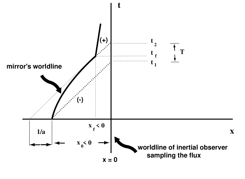
Figure 1: A moving mirror which emits delta function pulses of negative and positive energy. The mirror is initially at rest at $x=x_{0}$, and emits a negative energy pulse as it begins to accelerate with constant proper acceleration $a$. At time $t_{f}$ and position $x=x_{f}$, it ceases accelerating and emits a pulse of positive energy. An inertial observer at $x=0$ receives these pulses at $t=t_{1}$ and $t=t_{2}$, respectively.

In Ref. [18], it was shown that the magnitude of the $(-)$ energy pulse emitted by the mirror, $|\Delta E|$, is given by

$$|\Delta E|=\frac{a}{12\pi}\,,$$ (7)

and that the magnitude and the pulse separation, $T$, are constrained by the inequality

$$|\Delta E|\,T<\frac{1}{12\pi}\,.$$ (8)

For an observer to the right of the mirror, the energy flux is given by Eq. (2.24) of Ref. [18] with the sign of $V$ changed. From this expression, it can be shown that the magnitude of the positive pulse, $\Delta E_{p}$, is

$$\Delta E_{p}=\frac{a}{12\pi}\,\frac{\sqrt{1-V_{f}^{2}}}{{(1-V_{f})}^{2}}\,,$$ (9)

and therefore

$$1+\epsilon=\frac{(\Delta E_{p})}{|\Delta E|}=\frac{\sqrt{1-{V_{f}}^{2}}}{(1-V_{f})^{2}}\,,$$ (10)

where $\epsilon$ is the fraction by which the magnitude of the $(+)$ energy pulse overcompensates that of the $(-)$ energy pulse, and $V_{f}$ is the velocity of the mirror when the acceleration ceases.

We now want to express $\epsilon$ in terms of $|\Delta E|$ and $T$. From Fig. 1, it can be seen that

$$t_{2}=t_{f}+|x_{f}|=t_{f}-x_{f}\,,$$ (11)

and

$$t_{1}=|x_{0}|=-x_{0}\,,$$ (12)

where we have used the fact that the final position of the mirror when it stops accelerating, $x_{f}$, is negative because the mirror stays to the left of the observer. Using $T=t_{2}-t_{1}$, and Eq. (5), we obtain

$$t_{f}=\frac{T\,(aT-2)}{2(aT-1)}\,.$$ (13)

Equations (6),  (10),  (13), the fact that $aT<1$, and a straightforward but slightly tedious calculation imply

$$\epsilon=\frac{aT\,(2a^{2}\,T^{2}-5aT+4)}{2{(1-aT)}^{3}}\,.$$ (14)

If we rewrite this equation using Eq. (7), we get

$$\epsilon=\frac{24\,\pi|\Delta E|\,T\,(72\,{\pi}^{2}\,{|\Delta E|}^{2}\,T^{2}-15\,\pi\,|\Delta E|\,T+1)}{{(1-12\,\pi|\Delta E|\,T)}^{3}}\,,$$ (15)

which is a monotonically increasing function of $|\Delta E|\,T$. In the nonrelativistic, i. e., small $|\Delta E|\,T$, limit Eq. (15) becomes

$$\epsilon\approx 24\pi\,|\Delta E|\,T+504{\pi}^{2}\,{(|\Delta E|\,T)}^{2}+O[T^{3}]\dots\,.$$ (16)

The leading term on the right-hand side of this expression is identical to an earlier result derived in Sec. IIE of Ref. [19]. There only the nonrelativistic case was considered and the more general result, now confirmed by our Eq. (15) above, was conjectured.

In this simple example, it is easy to see why there is a maximum pulse separation, $T<T_{max}=1/(12\pi\,|\Delta E|)$, and how quantum interest arises. The former arises from the constraint that the mirror not collide with the observer. The latter is produced by the Doppler shifting of the $(+)$ energy pulse due to the nonzero velocity of the mirror when the pulse is emitted, i. e., at the moment when the mirror’s acceleration is halted. We speculated in Ref. [19] that quantum interest might be a more general phenomenon which generically occurs in cases of separated $\delta$-function pulses of $(-)$ and $(+)$ energy, in four as well as in two dimensions, regardless of how the pulses are produced. In the following sections of this paper, we will prove that this is in fact the case.

3 A General Constraint on Pulse Separations

In this section, we will show that quantum inequalities impose a maximum time separation, $T_{max}$, on any pair of $(-)$ and $(+)$ energy $\delta$-function pulses, in both two and four-dimensional flat spacetime. Let the pulse profile be given by

$$\rho(t)=B\,[-\delta(t)+(1+\epsilon)\,\delta(t-T)]\,,$$ (17)

where $B=|\Delta E|$ in two dimensions, and $B=|\Delta E|/A$ in four dimensions, where $A$ is the (planar) collecting area of the flux [34].

The quantum inequalities have the general form

$$\hat{\rho}=\int_{-\infty}^{\infty}\,g(t)\,\rho(t)\geq-\frac{C}{{t_{0}}^{D}}\,,$$ (18)

where $\rho(t)$ is the energy density, $g(t)$ is the sampling function, $C$ is a constant whose value depends on both the specific choice of sampling function and the spacetime dimension, $D$. Substituting Eq. (17) into Eq. (18), we obtain

$$\hat{\rho}=B\,[-g(0)+(1+\epsilon)\,g(T)]\geq-\frac{C}{{t_{0}}^{D}}\,.$$ (19)

Let us use a compactly-supported sampling function with width $t_{0}$, e. g., the sampling function vanishes (continuously) for $t\leq-t_{0}/2$ and for $t\geq t_{0}/2$. We will also assume, for the purposes of this discussion, that the sampling function has only one maximum in this interval. The left-hand side of Eq. (19) will be most negative when $T\geq t_{0}/2$, since $g(T)=0$ in this region. The bound can then be written as

$$B\leq\frac{C}{g(0)\,{t_{0}}^{D}}\,.$$ (20)

We may express $t_{0}$ as a multiple of $T$:

$$t_{0}=\kappa T\,,$$ (21)

where $\kappa\leq 2$, and then rewrite Eq. (20) as

$$B\leq\frac{C}{g(0)\,{\kappa}^{D}\,T^{D}}\,.$$ (22)

The best bound is obtained for $\kappa=2$, and is given by

$$B\leq\frac{C}{2^{D}\,T^{D}\,g(0)}\,.$$ (23)

For a sampling function with a single maximum, $g(0)\propto 1/{t_{0}}$, so let $g(0)=C_{0}/{t_{0}}=C_{0}/2T$, where $C_{0}$ is a constant whose value depends only on the form of the chosen sampling function (but not on the spacetime dimension, unlike $C$). Equation (23) now yields the constraint

$$B\,T^{D-1}\leq\frac{C}{2^{D-1}\,C_{0}}\,.$$ (24)

We thus have the following constraints on the pulse separation, $T$:

$$T\leq\frac{C}{2\,C_{0}\,|\Delta E|}\,,$$ (25)

and

$$T\leq\frac{1}{2}\,{\biggl{(}\frac{C\,A}{C_{0}\,|\Delta E|}\biggr{)}}^{1/3}\,,$$ (26)

in two and four dimensions, respectively. Therefore, the larger the magnitude of the $(-)$ energy pulse, the smaller is the allowed time separation between the pulses.

An example of a compactly-supported sampling function, which was given in Ref. [32], is

$$g(t)=\left\{\matrix{0\,,&\,\,t<-t_{0}/2\cr(1/t_{0})\,[1+{\rm cos}(2\pi t/t_{0})]\,,&\,-t_{0}/2\leq t\leq t_{0}/2\cr 0\,,&\,\,t>t_{0}/2}\right.\,.$$ (27)

For this function $C_{0}=2$, and in two dimensions $C=\pi/6$, which gives the following constraint on the maximum pulse separation $T_{max}$:

$$T_{max}=\frac{\pi}{24\,|\Delta E|}\approx\frac{0.131}{|\Delta E|}\,.$$ (28)

For the same function, $C={\pi}^{2}/16$ in four dimensions, and the analogous constraint is :

$$T_{max}={\biggl{(}\frac{\pi}{16}\biggr{)}}^{2/3}\,{\biggl{(}\frac{A}{|\Delta E|}\biggr{)}}^{1/3}\approx 0.338\,{\biggl{(}\frac{A}{|\Delta E|}\biggr{)}}^{1/3}\,.$$ (29)

Note that in two dimensions, the bound on $T_{max}$ given by Eq. (28) is larger than the bound ${|\Delta E|}T_{max}=1/(12\pi)\approx 0.027$, for the moving mirror case. It could be that there are other quantum states in two dimensions for which the value of $T_{max}$ lies between the moving mirror value and the bound given by Eq. (28). Alternatively, it may be that the moving mirror case comes close to the maximum allowed value of $T_{max}$ for any quantum state in two dimensions. If that is true, then perhaps other choices of compactly-supported sampling functions would lead to stronger bounds on $T_{max}$. Of the various sampling functions which we have examined, the best bound was obtained for Eq. (27). At present, this remains an open question .

4 Necessity of Quantum Interest

In this section we will establish the existence of quantum interest. The first subsection contains a simple argument which proves the necessity of quantum interest in four-dimensional flat spacetime, using the Lorentzian sampling function. The second subsection extends this argument to more general sampling functions in both two and four dimensions.

4.1 A Simple Argument in Four Dimensions

It will now be shown that quantum interest must exist for $\delta$-function pulses in four-dimensional flat spacetime. Here we will use the Lorentzian sampling function. The quantum inequality is

$$\hat{\rho}\geq-\frac{C}{{t_{0}}^{4}}\,,$$ (30)

where $C=3/(32\,\pi^{2})$ in the earlier version of Ref. [20], and $C=27/(2048\,\pi^{2})$ in the improved version of FE [31]. If we substitute Eq. (17), with $B=|\Delta E|/A$, into Eq. (30), the resulting inequality may be rewritten as

$$\hat{\rho}=\frac{|\Delta E|}{\pi\,A}\,\frac{(\epsilon\,\beta^{2}-1)}{\beta T\,(1+\beta^{2})}\geq-\frac{C}{{\beta}^{4}\,T^{4}}\,,$$ (31)

where

$$\beta=\frac{t_{0}}{T}\,.$$ (32)

A non-trivial inequality is obtained only for $\epsilon\beta^{2}-1<0$, i. e., $0\leq\beta<1/\sqrt{\epsilon}$. A slight rearrangement of Eq. (31) gives

$$|\Delta E|\,T\leq\biggl{(}\frac{C\pi A}{T^{2}}\biggr{)}\,F(\beta)\,,$$ (33)

with

$$F(\beta)=\frac{1+\beta^{2}}{\beta^{3}\,(1-\epsilon\beta^{2})}\,.$$ (34)

Note that if we set $\epsilon=0$, corresponding to exactly compensating pulses, then

$$F(\beta)=\frac{1+\beta^{2}}{\beta^{3}}\rightarrow 0\,,\,\,{\rm as}\,\,\beta\rightarrow\infty\,.$$ (35)

Since the quantum inequality must hold for any value of $\beta$, this would imply that $|\Delta E|\,T^{3}\rightarrow\nobreak 0$, i. e., either $|\Delta E|=0$ or $T=0$. In either case, there would be no non-trivial pulses. Therefore, $\epsilon>0$, i. e., we must have quantum interest in four-dimensional flat spacetime.

To get the tightest bound in Eq. (33), we should evaluate the right-hand side at the smallest value of the function $F(\beta)$. A calculation using the computer algebra program MACSYMA shows that the minimum of $F(\beta)$ is at

$$\beta=\beta_{m}=\sqrt{\frac{\sqrt{(1+\epsilon)(1+25\epsilon)}+1-5\epsilon}{6\epsilon}}\,.$$ (36)

If we let $y(\epsilon)=F(\beta_{m}(\epsilon))$, then $y(\epsilon)$ is a monotonically increasing function (as can be shown, for example, by graphing the function). Therefore, Eq. (33) can be written as

$$|\Delta E|\,T\leq\biggl{(}\frac{C\pi A}{T^{2}}\biggr{)}\,y(\epsilon)\,,$$ (37)

or, inverting the inequality, as

$$\epsilon\geq y^{-1}\,\biggl{(}\frac{|\Delta E|\,T^{3}}{C\pi A}\biggr{)}\,.$$ (38)

Since $y(\epsilon)$ is a monotonically increasing function, so is $y^{-1}$, hence the minimum allowed value of $\epsilon$ increases as $|\Delta E|\,T^{3}$ increases.

In the $\epsilon\rightarrow 0$ limit, $y(\epsilon)\sim 3\sqrt{3\epsilon}/2$, and so Eq. (37) can be inverted to yield

$$\epsilon\geq\frac{4}{27}\,{\biggl{(}\frac{|\Delta E|\,T^{3}}{C\pi A}\biggr{)}}^{2}\,,$$ (39)

i. e., $\epsilon$ grows as $T^{6}$ for fixed $|\Delta E|$ and $A$.

4.2 A More General Approach to Quantum Interest

In this section we will develop a more general formalism for obtaining lower bounds upon $\epsilon$. First, it is convenient to formulate the quantum inequalities in terms of sampling functions which are dimensionless functions of a dimensionless variable, $z=t/t_{0}$. Let

$$G(z)=t_{0}g(t)\,.$$ (40)

The quantum inequalities still take the form of Eq. (18), where the constant $C$ is

$$C=\frac{1}{24\,\pi}\,\int_{-\infty}^{\infty}\,\frac{[G^{\prime}(z)]^{2}}{G(z)}\,dz\,,$$ (41)

in two dimensions, and

$$C=\frac{1}{16\,{\pi}^{2}}\,\int_{-\infty}^{\infty}\,{\bigl{[}{G^{1/2}}^{\prime\prime}(z)\bigr{]}}^{2}\,dz\,,$$ (42)

in four dimensions. The lower bound on $\epsilon$ can be obtained from Eq. (19):

$$\epsilon\geq\frac{1}{g(T)}\,\biggl{(}g(0)-\frac{C}{B\,{t_{0}}^{D}}\biggr{)}-1\,.$$ (43)

In terms of $G$, this bound is

$$\epsilon\geq\frac{1}{G(x)}\,\biggl{[}C_{0}-\frac{C}{B}\,\biggl{(}\frac{x}{T}\biggr{)}^{D-1}\biggl{]}-1\,,$$ (44)

where $C_{0}=G(0)$ and

$$x=T/t_{0}\,.$$ (45)

We can express this as an upper bound on $T$ for fixed $\epsilon$ as

$$B\,T^{D-1}\leq H(x,\epsilon)\,,$$ (46)

where

$$H(x,\epsilon)=\frac{C\,x^{D-1}}{C_{0}-(\epsilon+1)G(x)}\,.$$ (47)

Note that our bound is nontrivial only if $C_{0}-(\epsilon+1)G(x)>0$.

The basic strategy which we will pursue is the following: first find the value $x=x_{m}$ which minimizes the function $H(x,\epsilon)$ for fixed $\epsilon$. Then the best bound on $T$ for a given form of $G$ is

$$B\,T^{D-1}\leq y(\epsilon)\equiv H(x_{m},\epsilon)\,.$$ (48)

If $y(\epsilon)$ is a monotonically increasing function, then so is its inverse $y^{-1}$, and we can write the lower bound on $\epsilon$ as

$$\epsilon\geq y^{-1}(B\,T^{D-1})\,.$$ (49)

The extremization with respect to $x$ is equivalent to that with respect to $\beta$ performed in the previous section, and amounts to finding the choice of sampling time which yields the strongest bound. If we set the first derivative of $H$ with respect to $x$ equal to zero, we find

$$(1+\epsilon)[xG^{\prime}-(D-1)G]+(D-1)C_{0}=0\,,$$ (50)

which is the equation to be solved for $x_{m}$. We will then need to check that $H^{\prime\prime}(x_{m})>0$ to verify that this is a minimum.

4.2.1 The Small $T$ Approximation

Let us first consider quantum interest in the small $T$ limit, which is determined by the behavior of $G(x)$ for small $x$. Take $G$ to be an even function which has the approximate form

$$G(z)\approx C_{0}-a\,z^{b}$$ (51)

for $0<z\ll 1$. If we substitute this form into Eq. (50) and solve the resulting equation, the result is

$$x_{m}=\left[\frac{(D-1)C_{0}\,\epsilon}{a(\epsilon+1)(D-b-1)}\right]^{\frac{1}{b}}\,.$$ (52)

The bound on $\epsilon$ in this case becomes

$$\epsilon\geq\frac{D-b-1}{C_{0}}\,\left(\frac{Bb}{C}\right)^{{b}/{(D-b-1)}}\,\left(\frac{a}{D-1}\right)^{{(D-1)}/{(D-b-1)}}\,T^{{b(D-1)}/{(D-b-1)}}\,.$$ (53)

As a check, we may compare this with the results of the previous subsection. Set $D=4$ and $b=2$ in the above bound, and then set $C_{0}=a=1/\pi$, corresponding to the Lorentzian sampling function. Then we obtain

$$\epsilon\geq\frac{4}{27\pi^{2}}\,\left(\frac{B}{C}\right)^{2}\,T^{6}\,,$$ (54)

which is equivalent to Eq. (39).

We need to check that $x=x_{m}$ is actually a minimum of $H$. For our procedure to be self-consistent, we must have $b<D-1$, as may be seen from Eq. (52). With this restriction it can be shown that $H^{\prime\prime}(x_{m},\epsilon)>0$, for this form of $G$. There is a further constraint on $b$ coming from the requirement that the integrals for $C$ converge at $x=0$, which requires that $b>\frac{1}{2}$ in two dimensions and $b>\frac{3}{2}$ in four dimensions. In two dimensions, the lower bound on $\epsilon$ from Eq. (53) grows as $T^{{b}/{(1-b)}}$ where $\frac{1}{2}<b<1$, and hence always grows faster than linearly for small $T$. In four dimensions, the corresponding bound grows as $T^{{3b}/{(3-b)}}$ where $\frac{3}{2}<b<3$, and hence grows faster than $T^{3}$ for small $T$. The main point of this calculation is to show that the quantum interest effect persists even in the limit of arbitrarily small temporal separation of the pulses. Note that this behavior is also a feature of the specific example of the moving mirror.

4.2.2 Numerical Bounds for General $T$

We can go beyond the small $T$ approximation by numerical methods. Here we restrict our discussion to a specific choice of sampling function,

$$G(z)=C_{0}\,e^{-|z|^{b}}\,,$$ (55)

for which

$$C_{0}=\frac{b}{2\Gamma(1/b)}\,.$$ (56)

This function has the form of Eq. (51) for $|z|\ll 1$, so the bounds obtained from it will be of the form of Eq. (53) for small $T$. Let us first use this sampling function to study quantum interest in two dimensions. Here Eq. (41) yields

$$C=\frac{b^{2}\,\Gamma((2b-1)/b)}{24\pi\Gamma(1/b)}\,,$$ (57)

and Eq. (50) becomes

$$e^{x^{b}}-(1+\epsilon)(bx^{b}+1)=0\,.$$ (58)

The root of this equation is $x=x_{m}$. The upper bound on $T$ for fixed $\epsilon$, Eq. (48), may now be expressed as

$$B\,T\leq\frac{C}{b\,C_{0}}\,x_{m}^{1-b}\,(1+bx_{m}^{b})\,.$$ (59)

For a given value of $b$, we may numerically solve Eq. (58) for fixed $\epsilon$, and check that $H^{\prime\prime}(x_{m},\epsilon)>0$. We then evaluate the right hand side of Eq. (59), which yields the limiting value of $T(\epsilon)$. The graph shown in Fig. 2 was obtained by inverting this relationship, and plotting $\epsilon(T)$. Typically,values of $b$ close to $\frac{1}{2}$ give the best bounds for small $T$. This is the case that was treated analytically above. Similarly, $b\approx 1.75$ gives the best bound for larger values of $T$. Larger values of $b$ actually give weaker bounds for $T<T_{max}$. Some results for various values of $b$ are given in Figure 2. Recall that Eq. (28) gives an upper bound on $T$ of $B\,T_{max}\approx 0.13$. For $T\approx T_{max}$, our sampling function requires that $\epsilon\geq\epsilon_{min}\approx 40$.

Figure 2: The lower bound on $\epsilon$ in two dimensions for different choices of $b$. Here the pulse separation $T$ is in units of $|\Delta E|^{-1}$.

A similar calculation may be performed in four dimensions. In this case

$$C=\frac{b^{2}\,(b-1)\,(2b-1)\,\Gamma((2b-3)/b)}{256\pi^{2}\Gamma(1/b)}\,,$$ (60)

the equation for $x_{m}$ is now

$$3\,e^{x^{b}}-(1+\epsilon)(bx^{b}+3)=0\,,$$ (61)

and the bound on $T$ is

$$T\leq\left[\frac{3C}{b\,B\,C_{0}}\,x_{m}^{3-b}\,(1+\frac{1}{3}bx_{m}^{b})\right]^{\frac{1}{3}}\,.$$ (62)

Again values of $b$ near the lower limit of $\frac{3}{2}$ give better bounds for small $T$, and larger values of $b$ give better bounds for larger $T$. Recall that Eq. (29) gives an upper bound on $T$ of $B^{\frac{1}{3}}\,T_{max}\approx 0.34$. The bounds which arise when $b=1.75$ and $b=2$ are shown in Figure 3. As in two dimensions, yet larger values of $b$ actually give weaker bounds for $T<T_{max}$.

Figure 3: The lower bound on $\epsilon$ in four dimensions for different choices of $b$. Here the pulse separation $T$ is in units of $(A/|\Delta E|)^{\frac{1}{3}}$.

5 Conclusions

We have proven that quantum states of the massless scalar field involving $\delta$-function pulses of $(-)$ and $(+)$ energy, in two and four-dimensional Minkowski spacetime, satisfy the “quantum interest conjecture.” This statement says that an energy “loan”, i. e., $(-)$ energy, must always be repaid, i. e., by $(+)$ energy, with an “interest” which increases with the magnitude and/or duration of the “loan.” Quantum interest is measured by the quantity $\epsilon$, which is the fraction by which the magnitude of the $(+)$ energy pulse overcompensates that of the $(-)$ energy pulse. A simple example of quantum interest, involving $\delta$-function pulses produced by a moving mirror, was examined in two-dimensional spacetime. There it was easy to see how quantum interest arose. It was the result of a Doppler-shifting of the subsequent $(+)$ energy pulse emitted by the mirror when its acceleration was brought to a stop in order to avoid a collision with the observer. The use of compactly-supported sampling functions enabled us to conclude that, for a fixed magnitude of the $(-)$ energy pulse, there must be a maximum allowed time separation between the pulses, in both two and four dimensions. This was deduced by placing the $(+)$ energy pulse in the region where the sampling function vanished. At present, we do not know what the optimal value of this separation might be. In two dimensions, we do know that it must be no smaller than $T=1/(12\,\pi|\Delta E|)$, so as to not rule out the moving mirror example. Another important question is which choice of sampling function maximizes quantum interest, for a fixed choice of $T$. These are unresolved problems to which we hope to return later.

Moving mirrors generate more quantum interest than is required by our bounds. For example, $\epsilon\approx 4$ at $T=1/(24\,\pi\,|\Delta E|)\approx 0.0133/|\Delta E|$, which is one-half of ${(T_{max})}_{mirror}$. This is much larger than the bounds on $\epsilon$ illustrated in Fig. 2. It may be that the moving mirror state generates much more quantum interest than similar quantum states in which the pulses are produced by other mechanisms. Alternatively, it may be that the moving mirror state is close to the generic case of quantum interest in two dimensions. In this event, presumably other choices of the sampling function would predict a value for $\epsilon$ which is much closer to the moving mirror value. At present, this question also remains unresolved.

Our central result is that quantum inequalities imply that quantum interest must exist for pulses in both two and four-dimensional flat spacetime. This takes the form of a lower bound on $\epsilon$ which is a monotonically increasing function of the pulse separation, for a fixed magnitude of the negative energy pulse. The bound is nonzero even for arbitrarily small pulse separations. Once again it appears that nature enforces rather strict constraints on manipulations of $(-)$ energies. The energy density integrated along an inertial observer’s worldline must be positive and the sampled energy density obeys the quantum inequalities. The degree of overcompensation by the $(+)$ energy increases with increasing pulse separation. In addition, there exists a maximum allowed pulse separation, which thereby limits the duration of the effects of the $(-)$ energy.

Acknowledgements

The authors would like to thank Michael J. Pfenning for useful discussions. TAR would like to thank the members of the Tufts Institute of Cosmology for their hospitality while this work was being done. This research was supported by NSF Grant No. Phy-9800965, and by a CCSU/AAUP faculty research grant.

References

- [1] S.W. Hawking and G.F.R. Ellis, The Large Scale Structure of Spacetime (Cambridge University Press, London, 1973), p. 88-96.
- [2] H. Epstein, V. Glaser, and A. Jaffe, Nuovo Cim. 36, 1016 (1965).
- [3] C. Kuo, Nuovo Cim. 112B, 629 (1997), gr-qc/9611064.
- [4] H.B.G. Casimir, Proc. K. Ned. Akad. Wet. B51, 793 (1948); L.S. Brown and G.J. Maclay, Phys. Rev. 184, 1272 (1969).
- [5] S.K. Lamoreaux, Phys. Rev. Lett. 78, 5 (1997).
- [6] U. Mohideen and A. Roy, Phys. Rev. Lett. 81, 4549 (1998), physics/9805038.
- [7] However, see A.D. Helfer and A.S.I.D. Lang, The Electromagnetic Field near a Dielectric Half-Space, hep-th/9810131.
- [8] L.-A. Wu, H.J. Kimble, J.L. Hall, and H. Wu, Phys. Rev. Lett. 57, 2520 (1986).
- [9] M. Alcubierre, Class. Quantum Grav. 11, L73 (1994).
- [10] S.V. Krasnikov, Phys. Rev. D 57, 4760 (1998), gr-qc/9511068.
- [11] M. Morris and K. Thorne, Am. J. Phys. 56, 395 (1988).
- [12] M. Morris, K. Thorne, and U. Yurtsever, Phys. Rev. Lett. 61, 1446 (1988).
- [13] S.W. Hawking, Phys. Rev. D 46, 603 (1992).
- [14] A.E. Everett, Phys. Rev. D 53, 7365 (1996).
- [15] L.H. Ford, Proc. Roy. Soc. Lond. A 364, 227 (1978).
- [16] P.C.W. Davies, Phys. Lett. 113B, 215 (1982).
- [17] L.H. Ford, Phys. Rev. D 43, 3972 (1991).
- [18] L.H. Ford and T.A. Roman, Phys. Rev. D 41, 3662 (1990).
- [19] L.H. Ford and T.A. Roman, Phys. Rev. D 46, 1328 (1992).
- [20] L.H. Ford and T.A. Roman, Phys. Rev. D 51, 4277 (1995), gr-qc/9410043.
- [21] L.H. Ford and T.A. Roman, Phys. Rev. D 55, 2082 (1997), gr-qc/9607003.
- [22] At first sight, one might think that the Casimir effect is a counterexample to the quantum inequalities. In fact, this is not quite correct. For details, see Refs. [20, 25, 27].
- [23] M.J. Pfenning and L.H. Ford, Phys. Rev. D 55, 4813 (1997), gr-qc/9608005.
- [24] D.-Y. Song, Phys. Rev. D 55, 7586 (1997), gr-qc/9704001.
- [25] M.J. Pfenning and L.H. Ford, Phys. Rev. D 57, 3489 (1998), gr-qc/9710055.
- [26] C.J. Fewster and E. Teo, Bounds on negative energy densities in static space-times, gr-qc/9812032.
- [27] L.H. Ford and T.A. Roman, Phys. Rev. D 53, 5496 (1996), gr-qc/9510071.
- [28] M.J. Pfenning and L.H. Ford, Class. Quantum Grav. 14, 1743 (1997), gr-qc/9702026.
- [29] A.E. Everett and T.A. Roman, Phys. Rev. D 56, 2100 (1997), gr-qc/9702026.
- [30] É. É. Flanagan, Phys. Rev. D 56, 4922 (1997), gr-qc/9706006.
- [31] C.J. Fewster and S.P. Eveson, Phys. Rev. D 58, 084010 (1998), gr-qc/9805024.
- [32] M.J. Pfenning, L.H. Ford, and T.A. Roman, Phys. Rev. D 57, 4839 (1998), gr-qc/9711030.
- [33] S.A. Fulling and P.C.W. Davies, Proc. R. Soc. London A348, 393 (1976); P.C.W. Davies and S.A. Fulling, ibid. A356, 237 (1977).
- [34] In this paper the area will be arbitrary. However, sometimes it is useful to impose the condition that all parts of the absorbing system come into causal contact with one another before the arrival of the positive energy. This implies . See Ref. [17] for a discussion of this point.