$SL(2,R)$ model with two Hamiltonian constraints

Abstract

We describe a simple dynamical model characterized by the presence of two noncommuting Hamiltonian constraints. This feature mimics the constraint structure of general relativity, where there is one Hamiltonian constraint associated with each space point. We solve the classical and quantum dynamics of the model, which turns out to be governed by an $SL(2,R)$ gauge symmetry, local in time. In classical theory, we solve the equations of motion, find a $SO(2,2)$ algebra of Dirac observables, find the gauge transformations for the Lagrangian and canonical variables and for the Lagrange multipliers. In quantum theory, we find the physical states, the quantum observables, and the physical inner product, which is determined by the reality conditions. In addition, we construct the classical and quantum evolving constants of the system. The model illustrates how to describe physical gauge-invariant relative evolution when coordinate time evolution is a gauge.

]

I Introduction

General relativity (GR) has a characteristic gauge invariance, which implies that its canonical Hamiltonian vanishes weakly. As a consequence, its dynamics is not governed by a genuine Hamiltonian, but rather by a “Hamiltonian constraint”. This peculiar feature of the theory has a crucial physical significance, connected to the relational nature of the general-relativistic spatiotemporal notions [1, 2, 3], and raises a number of important conceptual as well as technical problems, particularly in relation to the quantization of the theory [4]. In the past, much clarity has been shed on these problems by studying finite dimensional models mimicking the constraint structure of the theory, and in particular, having weakly vanishing Hamiltonian [3].

There is an aspect of the constraint structure of GR, however, which, as far as we are aware, has not been analyzed with the use of constrained models. In GR, there isn’t just a single Hamiltonian constraint, but rather a family of Hamiltonian constraints, one, so to say, for each coordinate-space point. Furthermore, the Hamiltonian constraints do not commute with each other (have nonvanishing Poisson brackets with each other). Indeed, the constraint algebra of GR has the well known structure

$$\{H,H\}\sim D,\ \ \ \{H,D\}\sim H,\ \ \ \{D,D\}\sim D,$$ (1)

where $H$ represents the Hamiltonian constraints and $D$ the diffeomorphism constraints. In this paper we present a model that mimics this aspect of GR.

The model we present has three constraints, which we call $H_{1}$, $H_{2}$ and $D$. Their algebra has the structure

$$\{H_{1},H_{2}\}\sim D,\ \ \ \{H_{i},D\}\sim H_{i},$$ (2)

which mimics (1). (Models with several commuting Hamiltonian constraints were considered in [5].) The constraints $H_{1}$ and $H_{2}$ are quadratic in the momenta, while $D$ is linear, as their correspondents in GR.

The model has an interesting structure which exemplifies in a non trivial manner various aspects of the quantization and interpretation of the fully constrained systems. We analyze in detail its classical and quantum dynamics, which can both be solved completely. We display the general solution of the equations of motion and the finite gauge transformation of variables and Lagrange multipliers. The constraint algebra turns out to be $SL(2,R)$ and the model is invariant under an $SL(2,R)$ gauge invariance, local in time. We find a complete $SO(2,2)$ algebra of gauge invariant observables, as well as a (smaller) complete set of independent observables. The phase space turns out to have the topology of four cones connected at their vertices. We then study the quantum dynamics, solve the Dirac constraints, exhibit the physical states explicitly, and construct a complete family of gauge invariant operators. The reality properties of the gauge invariant operators fix uniquely the physical scalar product. In addition, we define the classical and quantum evolving constants [6] of the system, and we discuss the observability of evolution for the systems (like GR) in which time is a gauge and the theory has no preferred physical time.

II Classical Dynamics

Definition of the model. The model we consider is defined by the action

$$S[{\vec{u}},{\vec{v}},N,M,\lambda]=\hskip 140.00021pt$$ (3)

$$\frac{1}{2}{\displaystyle\int}\ dt\left[\,N\,({\cal D}\vec{u}^{2}+\vec{v}^{2})+M\,({\cal D}\vec{v}^{2}+\vec{u}^{2})\,\right],$$ (4)

where

$${\cal D}{\vec{u}}=\frac{1}{N}(\dot{\vec{u}}-\lambda{\vec{u}}),\ \ \ \ \ {\cal D}{\vec{v}}=\frac{1}{M}(\dot{\vec{v}}+\lambda{\vec{v}});$$ (5)

the two Lagrangian dynamical variables ${\vec{u}}=(u^{1},u^{2})$ and ${\vec{v}}=(v^{1},v^{2})$ are two-dimensional real vectors; $N$, $M$ and $\lambda$ are Lagrange multipliers. The squares are taken in $R^{2}$: $\vec{u}^{2}=\vec{u}\cdot\vec{u}=(u^{1})^{2}+(u^{2})^{2}$.

Hamiltonian analysis. The Hamiltonian analysis is simplified by first rewriting the action in the following form

$$S = \int dt\left[\dot{\vec{u}}\cdot{\cal D}{\vec{u}}+\dot{\vec{v}}\cdot{\cal D}{\vec{v}}-N\frac{1}{2}({\cal D}{\vec{u}}^{2}-\vec{v}^{2})\right.$$ (7)

$$\left.\hskip 20.00003pt-M\frac{1}{2}({\cal D}{\vec{v}}^{2}-\vec{u}^{2})-\lambda({\vec{u}}\cdot{\cal D}{\vec{u}}-{\vec{v}}\cdot{\cal D}{\vec{v}})\right]\,.$$

From this form, we see that the momenta conjugate to $\vec{u}$ and $\vec{v}$ are

$${\vec{p}}={\cal D}{\vec{u}}\hskip 20.00003pt\mathrm{and}\hskip 20.00003pt{\vec{\pi}}={\cal D}{\vec{v}}$$ (8)

respectively, and that we have a weakly vanishing Hamiltonian and three primary constraints

$$H_{1} = \frac{1}{2}(\vec{p}^{2}-\vec{v}^{2})\,,$$ (9)

$$H_{2} = \frac{1}{2}(\vec{\pi}^{2}-\vec{u}^{2})\,,$$ (10)

$$D\ = {\vec{u}}\cdot{\vec{p}}-{\vec{v}}\cdot{\vec{\pi}}\,.$$ (11)

The Hamilton equations of motion are

$$\dot{\vec{u}}=N{\vec{p}}+\lambda{\vec{u}}\,, \dot{\vec{v}}=M{\vec{\pi}}-\lambda{\vec{v}}\,,$$ (12)

$$\dot{\vec{p}}=M{\vec{u}}-\lambda{\vec{p}}\,, \dot{\vec{\pi}}=N{\vec{v}}+\lambda{\vec{\pi}}\,.$$ (13)

Using (11) and (13) we find the evolution of the constraints

$${\dot{H}}_{1} = \ MD-2\lambda H_{1}\,,$$ (14)

$${\dot{H}}_{2} = -ND+2\lambda H_{2}\,,$$ (15)

$${\dot{D}}\ = -2MH_{2}+2NH_{1}\,.$$ (16)

These equations show that there are no secondary constraints, and that three constraints (11) are first class. The dynamics of the system is given entirely by the constraints and the Hamiltonian is $H=NH_{1}+MH_{2}+\lambda D$. Since we have four real dynamical variables ($\vec{u}$ and $\vec{v}$) and three first class constraints, the system has a single physical degree of freedom.

The Poisson algebra of the constraints can be read directly from (16); it is given by (cfr. eq. (2))

$$\{H_{1}\,,\,H_{2}\} = D\,,$$ (17)

$$\{H_{1}\,,\,D\}\, = -2H_{1}\,,$$ (18)

$$\{H_{2}\,,\,D\}\, = 2H_{2}\,.$$ (19)

This algebra is isomorphic to $sl(2,R)$, the Lie algebra of the group $SL(2,R)$.

Analogy with GR. The model has a structure recalling GR. The analogy is transparent in the Hamiltonian framework, given the similar structure of the two constraint algebras. In the Lagrangian framework, compare the action (4) with the Einstein-Hilbert action $S_{GR}$. Written in terms of the Arnowitt-Deser-Misner (ADM) variables, $S_{GR}$ is

$$S_{GR}[g,N,\lambda] = \int dt\int\sqrt{g}d\vec{x}\ N\,(Dg^{2}+R[g]),$$ (20)

$$Dg_{ab} = \frac{1}{N}(\dot{g}_{ab}-2D_{(a}\lambda_{b)})$$ (21)

where $g$ is the three-dimensional metric, $N$ the lapse and $\lambda$ the shift, $R$ the three-dimensional Ricci scalar, we have indicated the extrinsic curvature by $-Dg_{ab}$ and written $Dg^{2}\equiv Dg_{c}^{c}Dg_{d}^{d}-Dg_{ab}Dg^{ab}$. Notice that the two components of $\vec{u}$ mimic the metric in a space point, the two components of $\vec{v}$ mimic the metric in a second space point, $N$ mimics the lapse in the first point, $M$ the lapse in a second point and $\lambda$ the shift. The sum in (4) mimics the integration over $x$ in (21), and the definition of $D\vec{v}$ and $D\vec{v}$ mimics the extrinsic curvature.

Gauge invariance. Under an infinitesimal gauge transformation generated by infinitesimal time dependent parameters $n(t),m(t),l(t)$, the canonical variables transforms as [7]

$$\delta{\vec{u}} = l(t){\vec{u}}+n(t){\vec{p}}\,,$$ (22)

$$\delta{\vec{p}} = m(t){\vec{u}}-l(t){\vec{p}}\,,$$ (23)

$$\delta{\vec{\pi}} = l(t){\vec{\pi}}+n(t){\vec{v}}\,,$$ (24)

$$\delta{\vec{v}} = m(t){\vec{\pi}}-l(t){\vec{v}}\,,$$ (25)

while the Lagrange multipliers transform as [8]

$$\delta N = {\dot{n}}(t)-2n(t)\lambda+2l(t)N\,,$$ (26)

$$\delta M = {\dot{m}}(t)+2m(t)\lambda-2l(t)M\,,$$ (27)

$$\delta\lambda\ \, = \,{\dot{l}}(t)+n(t)M-m(t)N\,.$$ (28)

We can check the transformation of the action (7) under this infinitesimal variation of the canonical variables and the Lagrange multipliers. We find that $\delta S=0$ provided that the boundary term $n(t)(p^{2}+v^{2})+m(t)({\pi}^{2}+u^{2})|^{t=t_{f}}_{t=t_{i}}$ vanishes.

The problem of finding the finite gauge transformations can be solved by using the fact that (25) is an infinitesimal $SL(2,R)$ transformation. More precisely, each one of the four pairs $(u^{1},p^{1})$, $(u^{2},p^{2})$, $(\pi^{1},v^{1})$, $(\pi^{2},v^{2})$ (notice that the order is inverted in the second two), transforms in the fundamental representation of $SL(2,R)$. It follows that the finite gauge transformation of the canonical variables generated by the first class constraints are given by finite $SL(2,R)$ transformations as follows

$${\vec{u}}^{\prime}=\alpha(t){\vec{u}}+\beta(t){\vec{p}}\,, {\vec{\pi}}^{\prime}=\alpha(t){\vec{\pi}}+\beta(t){\vec{v}}\,,$$ (29)

$${\vec{p}}^{\prime}=\gamma(t){\vec{u}}+\delta(t){\vec{p}}\,, {\vec{v}}^{\prime}=\gamma(t){\vec{\pi}}+\delta(t){\vec{v}}\,,$$ (30)

where the matrix

$$G(t)=\pmatrix{\alpha(t)&\beta(t)\cr\gamma(t)&\delta(t)}$$ (31)

is in $SL(2,R)$, that is, with the only restriction that $\alpha(t)\delta(t)-\beta(t)\gamma(t)=1\,$. Thus, the system is invariant under an $SL(2,R)$ gauge invariance local in time.

The finite transformation law for the Lagrange multipliers can be found from the definitions of the momenta. We obtain with some algebra

$$N^{\prime} = \alpha^{2}N-\beta^{2}M-2\alpha\beta\lambda+\alpha{\dot{\beta}}-{\dot{a}}\beta\,,$$ (32)

$$M^{\prime} = -\gamma^{2}N+\delta^{2}M+2\gamma\delta\lambda+{\dot{\gamma}}\delta-\gamma{\dot{\delta}}\,,$$ (33)

$$\lambda^{\prime} = -\alpha\gamma N+\beta\delta M+(\alpha\delta+\beta\gamma)\lambda+{\dot{\alpha}}\delta-{\dot{\beta}}\gamma\,.$$ (34)

Below we give a clean geometric interpretation of these ugly-looking transformations.

We can now check the invariance of the action. By plugging (30) and (34) into the action (7) we get with some algebra

$$S^{\prime} = \int dt\left[{\dot{\vec{u}}}\cdot{\vec{p}}+{\dot{\vec{v}}}\cdot{\vec{\pi}}-(NH_{1}+MH_{2}+\lambda D)\right]+$$ (37)

$$\hskip 20.00003pt+\left[(\beta\gamma)({\vec{u}}\cdot{\vec{p}}+{\vec{v}}\cdot{\vec{\pi}})+\frac{1}{2}(\alpha\gamma)(u^{2}+{\pi}^{2})\right.$$

$$\hskip 20.00003pt\left.+\frac{1}{2}(\beta\delta)(p^{2}+v^{2})\right]^{t=t_{f}}_{t=t_{i}}\,.$$

The action is invariant provided that the boundary term vanishes.

Solution to the equations of motion. The evolution of the system can be viewed geometrically. Let us focus on the $(\vec{u},\vec{p})$ sector –the $(\vec{\pi},\vec{v})$ behaves in the same manner. The equations of motion (13) for this sector can be written in the form

$$\frac{d}{dt}\pmatrix{{\vec{u}}\cr{\vec{p}}\cr}-\pmatrix{\lambda&N\cr M&-\lambda}\pmatrix{{\vec{u}}\cr{\vec{p}}\cr}=0\,.$$ (38)

The matrix composed by the Lagrange multipliers is valued in the Lie Algebra of the $SL(2,R)$ group and can be viewed as the Yang-Mills connection for the local (in time) gauge group $SL(2,R)$

$$A(t)=\pmatrix{\lambda(t)&N(t)\cr M(t)&-\lambda(t)}\,.$$ (39)

This is not a vague analogy: using this notation, the ugly transformation (34) becomes

$$A^{\prime}=GAG^{-1}-G\frac{d}{dt}G^{-1}$$ (40)

That is, $A$ transforms precisely as a connection. Under a time dependent gauge transformation $G(t)$, $(\vec{u},\vec{p})$ transform as in (30), $A$ transforms as in (40) and the form of the equation of motion (38) is preserved.

Given the geometric analogy, it is easy to integrate the equations of motion. The Lagrange multipliers can be chosen as arbitrary functions of time, namely we can choose an arbitrary time dependent $sl(2,R)$ matrix $A(t)$. The solution of the equations of motion (38) is then obtained from the initial value $(u_{0},p_{0})$ at time $t=0$ by

$$\pmatrix{{\vec{u}}(t)\cr{\vec{p}}(t)\cr}=\pmatrix{a(t)&b(t)\cr c(t)&d(t)}\pmatrix{{\vec{u}}_{0}\cr{\vec{p}}_{0}\cr}\,,$$ (41)

where the matrix

$$U(t)=\pmatrix{a(t)&b(t)\cr c(t)&d(t)}$$ (42)

satisfies the parallel transport equation

$$\frac{d}{dt}U(t)-A(t)U(t)=0\,.$$ (43)

The solution is given by the time ordered exponential

$$U(t)={\cal P}e^{\int_{0}^{t}A(t^{\prime})dt^{\prime}}\,.$$ (44)

Alternatively, we can chose $U(t)$ as an arbitrary one parameter (differentiable) family of $SL(2,R)$ matrices, and compute the Lagrange multipliers by derivation. The dynamics of the $(\vec{\pi},\vec{v})$ sector is the same, with the same $U(t)$ (one has only to remember that $\vec{v}$ appears second in the $(\vec{\pi},\vec{v})$, unlikely $\vec{u}$). This gives the complete solution of the classical equations of motion.

In conclusion, the general solution of the Lagrange equations is

$$\vec{u}(t) = a(t)\vec{u}_{0}+b(t)\vec{p}_{0},$$ (45)

$$\vec{v}(t) = c(t)\vec{\pi}_{0}+d(t)\vec{v}_{0}.$$ (46)

with

$$a(t)d(t)-b(t)c(t)=1$$ (47)

and $(\vec{u}_{0},\vec{v}_{0},\vec{p}_{0},\vec{\pi}_{0})$ satisfying the constraints, that is $\vec{p}_{0}^{2}=\vec{v}_{0}^{2},\ \ \vec{\pi}_{0}^{2}=\vec{u}_{0}^{2}$ and $\vec{u}_{0}\cdot\vec{p}_{0}=\vec{v}_{0}\cdot\vec{\pi}_{0}$. The corresponding Lagrange multipliers are obtained from (43).

$$N(t) = \dot{b}(t)a(t)-\dot{a}(t)b(t)\,,$$ (48)

$$M(t) = \dot{c}(t)d(t)-\dot{d}(t)c(t)\,,$$ (49)

$$\lambda(t) = \dot{a}(t)d(t)-\dot{b}(t)c(t)\,.$$ (50)

As expected for a fully constrained system, a solution of the equations of motion is given by a one-parameter family of gauge transformations.

Let us construct the general solution in a given gauge. We consider the gauge $M=-1$, $N=+1$ and $\lambda=0$. The matrix $A$ is then the unit antisymmetric matrix (and time independent) and its holonomy $U(t)$ is the rotation matrix by an angle $t$. We still have three arbitrary gauge fixings to impose at $t=0$. We choose $\vec{u}^{2}=\vec{v}^{2}$, $\vec{u}\cdot\vec{p}=0$ and $u^{2}(0)=0$. Using the constraints and the general solution (46), we obtain

$${\vec{u}}(t) = (r\cos(\epsilon t)\,,\,r\sin(\epsilon t))\,,$$ (51)

$${\vec{v}}(t) = (r\cos{(\epsilon^{\prime}t+\phi)}\,,\,r\sin{(\epsilon^{\prime}t+\phi)})\,,$$ (52)

$${\vec{p}}(t) = (-r\epsilon\sin(\epsilon t)\,,\,r\epsilon\cos{(\epsilon t)})\,,$$ (53)

$${\vec{\pi}}(t) = (r\epsilon^{\prime}\sin{(\epsilon^{\prime}t+\phi)}\,,\,-r\epsilon^{\prime}\cos{(\epsilon^{\prime}t+\phi)})\,,$$ (54)

with $\epsilon=\pm 1$ and $\epsilon^{\prime}=\pm 1$. In this gauge, the two vectors $\vec{u}$ and $\vec{v}$ have the same length and rotate with the same angular speed, equal to one. Notice that the solution depends on two (continuous) parameters. $r\in R^{+}$ is the length of the vectors, and $\phi\in S_{1}$ is their relative angle at $t=0$. Since the space of solutions is two-dimensional, there is a single degree of freedom, as anticipated. In addition, there are the two discrete parameter $\epsilon$ and $\epsilon^{\prime}$. These distinguish four branches of the space of solutions, in which each of the two vectors rotate either clockwise or anti-clockwise.

III Observables

Dirac Observables. An observable is a function on the constraint surface that is invariant under the gauge transformations generated by all first class constraints. Equivalently, an observable is a function on the phase space which has weakly vanishing Poisson brackets with the first class constraints. To find gauge invariant observables, we can proceed as follows. As already noticed, (30) indicates that the four two-dimensional vectors $\vec{x}_{i}=(x_{i}^{1},x_{i}^{2}),\ \ i=1,2,3,4$

$$\vec{x}_{1}=\!\pmatrix{u^{1}\cr p^{1}}\!,\ \vec{x}_{2}=\!\pmatrix{u^{2}\cr p^{2}}\!,\ \vec{x}_{3}=\!\pmatrix{\pi^{1}\cr v^{1}}\!,\ \vec{x}_{4}=\!\pmatrix{\pi^{2}\cr v^{2}}$$

transform under gauge transformation in the fundamental representation of $SL(2,R)$. But $SL(2,R)$ preserves areas in $R^{2}$, that is, it preserves the vector product of any two vectors. It follows immediately that the six observables

$$O_{ij}=\vec{x}_{i}\times\vec{x}_{j}=x_{i}^{1}x_{j}^{2}-x_{i}^{2}x_{j}^{1},$$ (55)

are all gauge invariant. Explicitly:

$$O_{12}=u^{1}p^{2}-p^{1}u^{2}, O_{23}=u^{2}v^{1}-p^{2}\pi^{1},$$ (56)

$$O_{13}=u^{1}v^{1}-p^{1}\pi^{1}, O_{24}=u^{2}v^{2}-p^{2}\pi^{2},$$ (57)

$$O_{14}=u^{1}v^{2}-p^{1}\pi^{2}, O_{34}=\pi^{1}v^{2}-v^{1}\pi^{2}.$$ (58)

The Poisson brackets between the components of the $\vec{x}_{i}$ are

$$\{x_{i}^{1},x_{j}^{1}\}=0,\ \ \ \{x_{i}^{2},x_{j}^{2}\}=0,\ \ \ \{x_{i}^{1},x_{j}^{2}\}=g_{ij}.$$ (59)

where $g_{ij}$ is the diagonal matrix $[1,1,-1,-1]$. From this observation, it easy to compute the Poisson algebra of the $O_{ij}$ observables

$$\{O_{ij},O_{kl}\}=g_{ik}O_{jl}-g_{il}O_{jk}+g_{jl}O_{ik}-g_{jk}O_{il}.$$ (60)

Therefore the Poisson algebra of the six gauge invariant observables $O_{ij}$ is isomorphic to the Lie algebra of $SO(2,2)$.

Since the physical space is two-dimensional (1 degree of freedom), there are at most two independent continuous observables. Therefore there must be four relations between the six observables $O_{ij}$, when the constraints are imposed. These relations can be easily obtained by computing the observables $O_{ij}$ in the gauge (54) at $t=0$. In fact, a relation between gauge invariant quantities which is true in a particular gauge is also true in general. From (54) we have

$$O_{12}=\epsilon J\,,\ \ \hskip 20.00003pt O_{34}=\epsilon^{\prime}J\,,$$ (61)

$$O_{13}=J\cos\phi\,, O_{24}=\epsilon\epsilon^{\prime}J\cos\phi\,,$$ (62)

$$O_{14}=J\sin\phi\ \,, O_{23}=-\epsilon\epsilon^{\prime}J\sin\phi\,.$$ (63)

where we have introduced

$$J=r^{2}.$$ (64)

Clearly

$$\epsilon\ O_{34}\ \ \ = \ \epsilon^{\prime}\ O_{12}\,,$$ (65)

$$\epsilon\ O_{24}\ \ \ = \ \epsilon^{\prime}\ O_{13}\,,$$ (66)

$$\epsilon\ O_{23}\ \ \ = -\epsilon^{\prime}\ O_{14}\,,$$ (67)

$$O_{ij}O^{ij} = \ \ 0\,,$$ (68)

In the last equation, indices are raised with $g_{ij}$. Since the $O_{ij}$ are gauge invariant, these relations hold in general on the constraint surface.

Thus, the two continuous quantities $J\in R^{+},\phi\in S_{1}$ and two discrete quantity $\epsilon,\epsilon^{\prime}=\pm 1$, defined in general by (63), namely by

$$\epsilon = {u^{1}p^{2}-p^{1}u^{2}\over|u^{1}p^{2}-p^{1}u^{2}|}\,,$$ (69)

$$\epsilon^{\prime} = {\pi^{1}v^{2}-v^{1}\pi^{2}\over|\pi^{1}v^{2}-v^{1}\pi^{2}|}\,,$$ (70)

$$J = |u^{1}p^{2}-p^{1}u^{2}|\,,$$ (71)

$$\phi = \arctan{u^{1}v^{2}-p^{1}\pi^{2}\over u^{1}v^{1}-p^{1}\pi^{1}}\,,$$ (72)

are gauge invariant observables. They can be taken as coordinates of the physical gauge-invariant phase space. Using (60,63,68), straightforward algebra yields the physical Poisson brackets:

$$\{J,\phi\}=\epsilon\epsilon^{\prime}.$$ (73)

($\epsilon$ and $\epsilon^{\prime}$ commute with everything.) Notice that $J=0$ is a single point (whatever $\phi$, $\epsilon$ and $\epsilon^{\prime}$). Therefore the phase space has the topology of four cones connected at their vertices ($J=0$). See Figure 1.

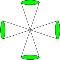
FIG. 1.: The topology of the phase space.

Notice that

$$O_{12} = \epsilon J=\vec{u}\times\vec{p}\,,$$ (74)

$$-O_{34} = -\epsilon^{\prime}J=\vec{v}\times\vec{\pi}\,.$$ (75)

are the “angular momenta” of the two two-dimensional “particles” $\vec{u}$ and $\vec{v}$. Since, from (65), $(O_{12})^{2}=(-O_{34})^{2}$, the two particles have the same “total angular momentum”. In the gauge (54), $\vec{u}$ and $\vec{v}$ rotate at equal angular speed: each one of the four cones represents an orientation of the two rotations, $J$ is their angular momentum and $\phi$ determines relative angle between $\vec{u}$ and $\vec{v}$.

The other four $O_{ij}$ arrange naturally in a $2\times 2$ matrix

$$M^{ab}\equiv\pmatrix{O_{13}&O_{14}\cr O_{23}&O_{24}}=u^{a}v^{b}-p^{a}\pi^{b},$$ (76)

where $a,b=1,2$. If we solve (46) for $a(t),b(t),c(t)$ and $d(t)$ and we insert the solution in (47), we obtain with some straightforward algebra

$$u^{a}(t)v^{b}(t)\ \epsilon_{ac}\epsilon_{bd}\ M^{cd}=O_{12}O_{34}.$$ (77)

(The $O_{ij}$ and $M^{cd}$ observables are time independent.) Using (63), this relation becomes

$$\left[u^{1}(t)v^{1}(t)+\epsilon\epsilon^{\prime}u^{2}(t)v^{2}(t)\right]\cos\phi$$ (78)

$$+\left[u^{1}(t)v^{2}(t)-\epsilon\epsilon^{\prime}u^{2}(t)v^{1}(t)\right]\sin\phi = J.$$ (79)

This is a key equation, which entirely captures the physical content of the model. It expresses the relation between the Lagrangian variables $(\vec{u},\vec{v})$ in each $(J,\phi,\epsilon,\epsilon^{\prime})$ state. The state of the system, $(J,\phi,\epsilon,\epsilon^{\prime})$, cannot be computed from the knowledge of the position $\vec{u},\vec{v}$ at a single time: two times, or a time derivative, are needed, as for any dinamical system. Once the state is determined, equation (79) provides us with the entire gauge invariant information: the relation between the Lagrangian variables at any other time.

We also define the two complex conjugate observables

$$R:=\epsilon Je^{i\phi} = \epsilon(O_{13}+iO_{14})=\epsilon^{\prime}(O_{24}-iO_{23}),$$ (80)

$$S:=\epsilon Je^{-i\phi} = \epsilon(O_{13}-iO_{14})=\epsilon^{\prime}(O_{24}+iO_{23}),$$ (81)

which will be convenient in the quantum theory. A complete set of observables is given by $J,R,S,\epsilon,\epsilon^{\prime}$ with the reality conditions

$$\overline{J}=J,\ \ \ \overline{R}=S.$$ (82)

Clearly

$$\cos\phi=\frac{1}{2\epsilon}(R+S)\ J^{-1},\ \ \ \sin\phi=\frac{1}{2i\epsilon}(R-S)\ J^{-1}.$$ (83)

Evolving constants. The physical phase space is the two-dimensional space of the gauge orbits on the constraint surface. A point in the physical phase space is determined by $(J,\phi,\epsilon,\epsilon^{\prime})$. This description of the system resolves gauge invariance, but looses reference to time evolution. Time evolution is, as in any fully constrained theory, a gauge transformation.

In certain fully constrained physical models such as the free relativistic particle or the Nambu string, there is a global implementation of the kinematical Poincaré group. The generator of this group that corresponds to the energy, can be taken as the physical Hamiltonian for time evolution. In other words, for these systems the natural time evolution can be introduced in the frozen reduced phase space by using the energy as Hamiltonian. This provides a preferred variable that plays the role of time, namely of the independent evolution parameter. Instead, the kinematical group is absent in GR (unless additional structure, such as flat asymptotic infinity is added), or in the model studied in this paper. In these cases, there is no preferred time variable. The theory just describes –very democratically !– the relative evolution of the variables, as functions of each other, without privileging any variable as the independent one. For a detailed discussion of the physical meaning of this very important feature of GR, see [2].

One way to express evolution in these cases, is to break gauge invariance. For instance, one can impose a time dependent gauge fixing (the analog of $x^{0}=t$ for a relativistic particle), or choose a gauge at time zero and then evolve with arbitrarily fixed Lagrange multipliers. This amounts to arbitrarily choosing one of the variables as the time variable.

Is there, in alternative, a gauge invariant description of time evolution? Are there gauge invariant observables that capture the dynamics of the Lagrangian variables $\vec{u}(t),\vec{v}(t)$? Can we talk about a gauge-invariant dynamics, if the time dependence of $\vec{u}(t)$ and $\vec{v}(t)$ is a gauge transformation? The answer is yes [6].

In fact, the gauge invariant (or physical) content of the model is not the description of the evolution of the 4 real variables $u^{1}(t),u^{2}(t),v^{1}(t),v^{2}(t)$ in the coordinate time $t$, but rather the description of their evolution as functions of each other. More precisely, since there are 4 variables and the gauge orbits are 3-dimensional, the system describes the motion of any one of these four variables as function of the other three. In other words, once the state of the system is known, the dynamical model allows us to predict the value of any one of the four Lagrangian variables from the value of the other three. This prediction is univocal and gauge-invariant.

Each solution of the classical system, namely each point of the phase space determines one functional relation between the four variables $u^{1}(t),u^{2}(t),v^{1}(t),v^{2}(t)$. This functional relation allows us to compute one of these variables from the value of the other three. This functional relation is given by equation (79).

The form of a gauge invariant observable describing evolution is therefore the following. Let us ask what is the value $U^{1}$ of the observable $u^{1}$, when $u^{2}$ and $\vec{v}$ have assigned values $u^{2}=x,v^{1}=y$ and $v^{2}=z$. In other words, we search an observable of the form $U^{1}=U^{1}(x,y,z;J,\phi,\epsilon,\epsilon^{\prime})$. Solving (79) for $u^{1}$, and replacing $u^{2},v^{1}$ and $v^{2}$ with $x,y$ and $z$, we obtain

$$U^{1}(x,y,z;J,\phi,\epsilon,\epsilon^{\prime})={-\epsilon^{\prime}x(z\cos\phi-y\sin\phi)+\epsilon J\over\epsilon(y\cos\phi+z\sin\phi)}.$$ (84)

This is an “evolving constant” in the sense of reference [6]. For any fixed state $(J,\phi,\epsilon,\epsilon^{\prime})$, the quantity $U^{1}(x,y,z;J,\phi,\epsilon,\epsilon^{\prime})$, viewed as a function of $x,y$ and $z$ gives the evolution of $u^{1}$ as a function of the other variables. Viceversa, for any fixed $x,y,z$, the quantity $U^{1}(x,y,z;J,\phi,\epsilon,\epsilon^{\prime})$, viewed as a function of $J,\phi,\epsilon$ and $\epsilon^{\prime}$, defines a gauge invariant function on the physical phase space. Similar expressions can be derived from (79) for $u^{2},v^{1}$ and $v^{2}$.

$$U^{2}(s,y,z;J,\phi,\epsilon,\epsilon^{\prime})\!\! = \!\!{-\epsilon s(y\cos\phi+z\sin\phi)+\epsilon J\over\epsilon^{\prime}(z\cos\phi-y\sin\phi)}\,,$$ (85)

$$V^{1}(s,x,z;J,\phi,\epsilon,\epsilon^{\prime})\!\! = \!\!{-z(\epsilon^{\prime}x\cos\phi+\epsilon s\sin\phi)+\epsilon J\over\epsilon s\cos\phi-\epsilon^{\prime}x\sin\phi}\,,$$ (86)

$$V^{2}(s,x,y;J,\phi,\epsilon,\epsilon^{\prime})\!\! = \!\!{-y(\epsilon s\cos\phi-\epsilon^{\prime}x\sin\phi)+\epsilon J\over\epsilon^{\prime}x\cos\phi+\epsilon s\sin\phi}\,,$$ (87)

where $s$ is the value of $u^{1}$. These observables describe the evolution of the system and are gauge invariant.

Time reparametrization invariance. The system is invariant under time reparametrization. If $(\vec{u}(t),\vec{v}(t))$ is a solution of the equations of motion, then

$$\pmatrix{\vec{u}^{\prime}(t)\cr\vec{v}^{\prime}(t)}=\pmatrix{\vec{u}(f(t))\cr\vec{v}(f(t))}$$ (88)

is also a solution. This is immediately seen from (46) and (47), because $a(f(t))d(f(t))-b(f(t))c(f(t))=1$ follows from $a(t)d(t)-b(t)c(t)=1$.

Notice that there exist gauges in which $\vec{u}(t)$ evolves in $t$ while $\vec{v}(t)$ remains constant. For instance we can choose $M=\lambda=0$. In this gauge,

$$A=\pmatrix{0&N(t)\cr 0&0}$$ (89)

and therefore

$$U(t)=\pmatrix{1&b(t)\cr 0&1}$$ (90)

so that

$${\vec{u}} = \vec{u}_{0}+b(t)\vec{p}_{0},$$ (91)

$${\vec{v}} = \vec{v}_{0}$$ (92)

with $N=\dot{b}$. A different example is the following. The solution (54) can be gauge transformed to the solution

$${\vec{u}}=(u\cos{t}\,,\,u\sin{t})\,,\ \ \ \ {\vec{v}}=(u\,,\,0)\,,$$ (93)

$${\vec{p}}=\left(u\frac{(\cos{t}-1)}{\sin{t}}\,,\,u\right)\,, {\vec{\pi}}=(u\sin{t}\,,\,0)\,,$$ (94)

where the Lagrange multipliers are $\lambda=\frac{\cos{t}-1}{\sin{t}}$, $M=-\frac{(\cos{t}-1)}{(\sin{t})^{2}}$, and $N=1$. Similarly, there is a gauge in which $\vec{v}(t)$ evolves in $t$ while $\vec{u}(t)$ remains constant.

Notice, however, that there isn’t really a “two finger time reparametrization invariance” in the system [5], in the sense that it is not true that if $(\vec{u}(t),\vec{v}(t))$ is a solution of the equations of motion, then

$$\pmatrix{\vec{u}^{\prime}(t)\cr\vec{v}^{\prime}(t)}=\pmatrix{\vec{u}(f_{1}(t))\cr\vec{v}(f_{2}(t))}$$ (95)

is also a solution. In fact, in any given time $\vec{u}^{\prime}(t)$ and $\vec{v}^{\prime}(t)$ must be connected to the same point in phase space by a gauge transformation, but in general it is not true that $a(f_{1}(t))d(f_{2}(t))-b(f_{1}(t))c(f_{2}(t))=1$ when $a(t)d(t)-b(t)c(t)=1$.

IV Quantum Dynamics

We work in the coordinate representation. Elements of the Hilbert space are functions $\Psi({\vec{u}},{\vec{v}})$ of the coordinates, and the momentum operators are

$${\widehat{\vec{p}}}=-i\hbar\vec{\nabla}_{u},\ \ \ {\widehat{\vec{\pi}}}=-i\hbar\vec{\nabla}_{v}.$$ (96)

By inserting these operators in the constraints we obtain the Dirac quantum constraints

$${\widehat{H}}_{1} = -\frac{1}{2}\left({\hbar}^{2}\Delta_{u}+\vec{v}^{2}\right)\,,$$ (97)

$${\widehat{H}}_{2} = -\frac{1}{2}\left({\hbar}^{2}\Delta_{v}+\vec{u}^{2}\right)\,,$$ (98)

$${\widehat{D}}\ = -i\hbar\left({\vec{u}}\cdot\vec{\nabla}_{u}-{\vec{v}}\cdot\vec{\nabla}_{v}\right)\,.$$ (99)

where $\Delta_{u}=\vec{\nabla}_{u}^{2}={\partial^{2}\over\partial{(u^{1})^{2}}}\ +{\partial^{2}\over\partial{(u^{2})^{2}}}$. In the Hamiltonian constraint operators ${\widehat{H}}_{1}$ and ${\widehat{H}}_{2}$ there is a natural ordering. In the “diffeomorphism” operator ${\widehat{D}}$, we have chosen the ordering that leads to the closure of the constraint algebra and thus the absence of anomalies. We have in fact

$$\left[{\widehat{H}}_{1}\,,\,{\widehat{H}}_{2}\right] = \ i\hbar{\widehat{D}}\,,$$ (100)

$$\left[{\widehat{H}}_{1}\,,\,{\widehat{D}}\right]\ = -2i\hbar{\widehat{H}}_{1}\,,$$ (101)

$$\left[{\widehat{H}}_{2}\,,\,{\widehat{D}}\right]\ = \ 2i\hbar{\widehat{H}}_{2}\,.$$ (102)

The physical states, in the sense of Dirac, are in the kernel of all the quantum constraints. Namely, they are defined by

$$\left({\hbar}^{2}\Delta_{u}+\vec{v}^{2}\right)\Psi({\vec{u}},{\vec{v}}) = 0\,,$$ (103)

$$\left({\hbar}^{2}\Delta_{v}+\vec{u}^{2}\right)\Psi({\vec{u}},{\vec{v}}) = 0\,,$$ (104)

$$-i\hbar\left({\vec{u}}\cdot\vec{\nabla}_{u}-{\vec{v}}\cdot\vec{\nabla}_{v}\right)\Psi({\vec{u}},{\vec{v}}) = 0\,.$$ (105)

We now solve this system of coupled partial differential equations.

We transform to polar coordinates

$${\vec{u}}=(u\cos{\alpha},\ \ u\sin{\alpha}){\hbox{, }}\vec{v}=(v\cos{\beta},v\sin{\beta})$$ (106)

and we multiplying the first equation of the system by $u^{2}/\hbar^{2}$ and the second by $v^{2}/\hbar^{2}$. (105) becomes

$$\left(u\frac{\partial}{\partial u}u\frac{\partial}{\partial u}+\frac{\partial^{2}}{\partial\alpha^{2}}+\frac{u^{2}v^{2}}{\hbar^{2}}\right)\Psi(u,v,\alpha,\beta) = 0\,,$$ (107)

$$\left(v\frac{\partial}{\partial v}v\frac{\partial}{\partial v}+\frac{\partial^{2}}{\partial\beta^{2}}+\frac{u^{2}v^{2}}{\hbar^{2}}\right)\Psi(u,v,\alpha,\beta) = 0\,,$$ (108)

$$\left(u\frac{\partial}{\partial u}-v\frac{\partial}{\partial v}\right)\Psi(u,v,\alpha,\beta) = 0\,.$$ (109)

We search a solution by separation of variables, by writing

$$\Psi(u,v,\alpha,\beta)=A(\alpha)\ B(\beta)\ \psi(u,v).$$ (110)

The first two equations in (109) give immediately

$$A(\alpha)=e^{im_{\alpha}\alpha},\ \ \ \ B(\beta)=e^{im_{\beta}\beta},$$ (111)

where $m_{\alpha}$ and $m_{\beta}$ must be integer for $\Psi$ to be continuous. The third equation in (109) implies that

$$\psi(u,v)=\psi(uv)$$ (112)

(a function of the product $uv$). Plugging this last result back into the first two equations in (109), we find that the first and last terms of one equation are equal to the first and last terms of the second. Therefore the two middle terms must be equal as well. Therefore the two equations imply $m^{2}_{\alpha}=m^{2}_{\beta}$. We put

$$m_{\alpha}=\epsilon m,\ \ \ \ m_{\beta}=-\epsilon^{\prime}m,\ \ \ \epsilon,\epsilon^{\prime}=\pm 1,$$ (113)

with $m$ any nonnegative integer. The minus is inserted for later convenience. Using this, the first two equations of the system become equal to each other and reduce to

$$\frac{d^{2}f(x)}{dx^{2}}+\frac{1}{x}\frac{df(x)}{dx}+\left(1-\frac{m^{2}}{x^{2}}\right)f(x)=0\,,$$ (114)

where we have written $x=uv/\hbar$ and $f(x)=\psi({\hbar}x)$. This is the Bessel equation. Thus, we have solved the system entirely. We conclude that the physical Hilbert space is spanned by the basis states $|m,\epsilon,\epsilon^{\prime}\rangle$, where $m$ is a nonnegative integer and $\epsilon,\epsilon^{\prime}=\pm 1$. In the coordinate representation these states are given by

$$\langle u,v,\alpha,\beta|m,\epsilon,\epsilon^{\prime}\rangle = \Psi_{m,\epsilon,\epsilon^{\prime}}(u,v,\alpha,\beta)$$ (115)

$$= e^{im(\epsilon\alpha-\epsilon^{\prime}\beta)}\ J_{m}\left(\frac{uv}{\hbar}\right)\,,$$ (116)

where $J_{m}$ is the Bessel function of order $m$. Notice that for each $m>0$ there are four states ($\epsilon=\pm 1,\epsilon^{\prime}=\pm 1$), but for $m=0$ there is only one state, since $|m,+,+\rangle=|m,+,-\rangle=|m,-,+\rangle=|m,-,-\rangle$ .

Quantum observables and scalar product. Consider the observables $O_{ij}$ defined in (58). They are gauge invariant, and thus have vanishing Poisson brackets with the constraints. We chose the natural ordering for the corresponding quantum operators $\hat{O}_{ij}$

$$\hat{O}_{12}=\hat{u}^{1}\hat{p}^{2}-\hat{p}^{1}\hat{u}^{2},\hskip 20.00003pt \hat{O}_{23}=\hat{u}^{2}\hat{v}^{1}-\hat{p}^{2}\hat{\pi}^{1},$$ (117)

$$\hat{O}_{13}=\hat{u}^{1}\hat{v}^{1}-\hat{p}^{1}\hat{\pi}^{1},\hskip 20.00003pt \hat{O}_{24}=\hat{u}^{2}\hat{v}^{2}-\hat{p}^{2}\hat{\pi}^{2},$$ (118)

$$\hat{O}_{14}=\hat{u}^{1}\hat{v}^{2}-\hat{p}^{1}\pi^{2},\hskip 20.00003pt \hat{O}_{34}=\hat{\pi}^{1}\hat{v}^{2}-\hat{v}^{1}\hat{\pi}^{2}.$$ (119)

It is easy to see that the commutators of these operators with the quantum constraints (99) vanish. Therefore these operators are well defined on the space of the solutions of the quantum constraints, namely on the states (116). We compute their action on these states. Going to polar coordinates we see immediately that

$$\hat{O}_{12}\ \Psi_{m,\epsilon,\epsilon^{\prime}} = -i\hbar\frac{\partial}{\partial\alpha}\Psi_{m,\epsilon,\epsilon^{\prime}}=\epsilon m\hbar\ \Psi_{m,\epsilon,\epsilon^{\prime}},$$ (120)

$$\hat{O}_{34}\ \Psi_{m,\epsilon,\epsilon^{\prime}} = \ \ i\hbar\frac{\partial}{\partial\beta}\Psi_{m,\epsilon,\epsilon^{\prime}}=\epsilon^{\prime}m\hbar\ \Psi_{m,\epsilon,\epsilon^{\prime}}.$$ (121)

Thus in the physical state space we have $\epsilon^{\prime}\hat{O}_{12}=\epsilon\hat{O}_{34}$: the relation between the two is precisely the same as in the classical theory, eq. (65). We can thus identify the $\epsilon$ and $\epsilon^{\prime}$ appeared in the quantum theory with the $\epsilon$ and $\epsilon^{\prime}$ appeared in solving the classical theory, and we conclude, from equation (63), that the quantum operator corresponding to the gauge invariant observable $J$ is

$$\hat{J}\ |m,\epsilon,\epsilon^{\prime}\rangle=\hbar m\ |m,\epsilon,\epsilon^{\prime}\rangle.$$ (122)

Thus in the quantum theory $J$ is discrete, quantized in multiples of $\hbar$

$$J=m\ \hbar.$$ (123)

Using the Bessel equation and the properties

$$J_{m-1}(x) = \frac{m}{x}J_{m}(x)+\frac{d}{dx}J_{m}(x),$$ (124)

$$J_{m+1}(x) = \frac{m}{x}J_{m}(x)-\frac{d}{dx}J_{m}(x)$$ (125)

of the Bessel functions, a straightforward but long calculation yields

$$(\hat{O}_{13}+i\hat{O}_{14})\ \Psi_{m,\epsilon,\epsilon^{\prime}} = \epsilon\hbar m\ \Psi_{m+\epsilon\epsilon^{\prime},\epsilon,\epsilon^{\prime}},$$ (126)

$$(\hat{O}_{24}-i\hat{O}_{23})\ \Psi_{m,\epsilon,\epsilon^{\prime}} = \epsilon^{\prime}\hbar m\ \Psi_{m+\epsilon\epsilon^{\prime},\epsilon,\epsilon^{\prime}}.$$ (127)

Thus, the quantum operator corresponding to the observable $R$ defined in (80) is

$$\hat{R}\ |m,\epsilon,\epsilon^{\prime}\rangle=\hbar m\ |m+\epsilon\epsilon^{\prime},\epsilon,\epsilon^{\prime}\rangle.$$ (128)

In the same manner, from (81) we obtain

$$\hat{S}\ |m,\epsilon,\epsilon^{\prime}\rangle=\hbar m\ |m-\epsilon\epsilon^{\prime},\epsilon,\epsilon^{\prime}\rangle.$$ (129)

To complete the construction of the Hilbert space of the physical quantum states, we have to determine the scalar product on the space spanned by the states $|m,\epsilon,\epsilon^{\prime}\rangle$. This is determined by the requirement that real classical observables be self adjoint. The observables $J,\epsilon$ and $\epsilon^{\prime}$ are real, and thus we require $\hat{J},\hat{\epsilon}$ and $\hat{\epsilon}^{\prime}$ to be self adjoint. It follows that the states $|m,\epsilon,\epsilon^{\prime}\rangle$ which are their eigenstates must form an orthogonal basis. This fixes the scalar product up to the norm of the basis states. Define

$$\langle m,\epsilon,\epsilon^{\prime}|m,\epsilon,\epsilon^{\prime}\rangle=c_{m,\epsilon,\epsilon^{\prime}}.$$ (130)

Next, $S$ is the complex conjugate of $R$. Thus we require that $R^{\dagger}=\hat{S}$. It follows

$$\langle m,\epsilon,\epsilon^{\prime}|\ R^{\dagger}\ |n,\epsilon,\epsilon^{\prime}\rangle=\langle m,\epsilon,\epsilon^{\prime}|\ \hat{S}\ |n,\epsilon,\epsilon^{\prime}\rangle.$$ (131)

From which, we have easily

$$c_{m,\epsilon,\epsilon^{\prime}}=cm.$$ (132)

Here $c$ is a positive overall normalization constant that has no effect on the physics, and we chose equal to 1. This fixes the normalization of the orthogonal basis states, and therefore determines the scalar product completely. Notice that the state $|0,\epsilon,\epsilon^{\prime}\rangle$ has zero norm. (This was first realized by Jorma Louko). We can therefore discard it, because its presence has no physical consequences. More precisely, we identify the $m=0$ state with the state zero.

The peculiar behavior of the $m=0$ sector of the quantum theory reflects the pathological properties of the corresponding classical state. The quantum state $m=0$ has vanishing angular momentum $J$; the classical state with vanishing angular momentum is the (common) vertex of the four cones that form the reduced phase space (see Figure 1). This is a point at which the reduced phase space fails to be a manifold. Physically, this corresponds to the fact that small perturbations of the $J=0$ solution form disjoint spaces.

Thus, the quantum theory is completely defined by the states

$$|\psi\rangle=\sum_{m=1,\infty;\epsilon,\epsilon^{\prime}=\pm}\ c_{m,\epsilon,\epsilon^{\prime}}\ |m,\epsilon,\epsilon^{\prime}\rangle,$$ (133)

the scalar product

$$\langle m,\epsilon,\epsilon^{\prime}|\tilde{m},\tilde{\epsilon},\tilde{\epsilon}^{\prime}\rangle=m\ \delta_{m,\tilde{m}}\delta_{\epsilon,\tilde{\epsilon}}\delta_{\epsilon^{\prime},\tilde{\epsilon}^{\prime}},$$ (134)

and the operators

$$\hat{J}\ |m,\epsilon,\epsilon^{\prime}\rangle = \hbar m\ |m,\epsilon,\epsilon^{\prime}\rangle,$$ (135)

$$\hat{R}\ |m,\epsilon,\epsilon^{\prime}\rangle = \hbar m\ |m+\epsilon\epsilon^{\prime},\epsilon,\epsilon^{\prime}\rangle,$$ (136)

$$\hat{S}\ |m,\epsilon,\epsilon^{\prime}\rangle = \hbar m\ |m-\epsilon\epsilon^{\prime},\epsilon,\epsilon^{\prime}\rangle,$$ (137)

$$\hat{\epsilon}\ |m,\epsilon,\epsilon^{\prime}\rangle = \epsilon\ \ |m,\epsilon,\epsilon^{\prime}\rangle,$$ (138)

$$\hat{\epsilon}^{\prime}\ |m,\epsilon,\epsilon^{\prime}\rangle = \epsilon^{\prime}\ |m,\epsilon,\epsilon^{\prime}\rangle.$$ (139)

where it is understood that $|0,\epsilon,\epsilon^{\prime}\rangle=0$. (That is, for instance, $\hat{R}\ |1,+,-\rangle=0$).

Quantum evolving constants. In order to quantize the evolving constant of motion (84,87), we must construct the operators corresponding to the classical observables $\cos\phi$ and $\sin\phi$. We denote these operators $\widehat{\cos\phi}$ and $\widehat{\sin\phi}$, with a slight abuse in notation. (The operator $\hat{\phi}$ is ill defined because $\phi$ is an angle –see for instance [9]– and we must deal with periodic functions of $\phi$ in order to have continuity all around the circle.) Choosing the natural ordering given in (83), we have immediately

$$\widehat{\cos\phi}\ |m,\epsilon,\epsilon^{\prime}\rangle = \frac{1}{2\epsilon}(|m+\epsilon\epsilon^{\prime},\epsilon,\epsilon^{\prime}\rangle+|m-\epsilon\epsilon^{\prime},\epsilon,\epsilon^{\prime}\rangle),$$ (140)

$$\widehat{\sin\phi}\ |m,\epsilon,\epsilon^{\prime}\rangle = \frac{1}{2\epsilon i}(|m+\epsilon\epsilon^{\prime},\epsilon,\epsilon^{\prime}\rangle-|m-\epsilon\epsilon^{\prime},\epsilon,\epsilon^{\prime}\rangle)$$ (141)

(where, again, it is understood that $|0,\epsilon,\epsilon^{\prime}\rangle=0$.)

A convenient representation of the theory can be obtained by representing a generic state

$$|\psi\rangle=\sum_{m,\epsilon,\epsilon^{\prime}}\psi_{m,\epsilon,\epsilon^{\prime}}\ |m,\epsilon,\epsilon^{\prime}\rangle$$ (142)

by the four functions on $S_{1}$

$$\psi_{\epsilon,\epsilon^{\prime}}(\phi)=\sum_{m=1}^{\infty}\psi_{m,\epsilon,\epsilon^{\prime}}\ e^{i\epsilon\epsilon^{\prime}m(\phi+\frac{\pi}{2}(3+\epsilon))}.$$ (143)

The scalar product turns out to be

$$\langle\psi_{\epsilon,\epsilon^{\prime}}|\tilde{\psi}_{\epsilon,\epsilon^{\prime}}\rangle=-i\epsilon\epsilon^{\prime}\int d\phi\ \bar{\psi}_{\epsilon,\epsilon^{\prime}}(\phi)\ \frac{d}{d\phi}\ \tilde{\psi}_{\epsilon,\epsilon^{\prime}}(\phi).$$ (144)

Notice that since the sum in (143) is restricted to $m>0$, the Hilbert space is formed by “right moving” functions $\psi_{+,+}(\phi)$ and $\psi_{-,-}(\phi)$, and “left moving” functions $\psi_{+,-}(\phi)$ and $\psi_{-,+}(\phi)$ only. On these functions, the scalar product (144) is positive definite. In particular, the zero modes $\psi_{\epsilon,\epsilon^{\prime}}(\phi)=constant$ do not belong to the Hilbert space. We denote the projector that projects out the zero modes as $P$. The observables are then

$$\hat{J}\ \ \psi_{\epsilon,\epsilon^{\prime}}(\phi) = -i\hbar\epsilon\epsilon^{\prime}\,\frac{d}{d\phi}\psi_{\epsilon,\epsilon^{\prime}}(\phi),$$ (145)

$$\widehat{\cos\phi}\ \psi_{\epsilon,\epsilon^{\prime}}(\phi) = P\ \cos\phi\ \psi_{\epsilon,\epsilon^{\prime}}(\phi),$$ (146)

$$\widehat{\sin\phi}\ \psi_{\epsilon,\epsilon^{\prime}}(\phi) = P\ \sin\phi\ \psi_{\epsilon,\epsilon^{\prime}}(\phi).$$ (147)

In this representation it is easy to write the quantum operator corresponding to the evolving constant of motion, which quantizes the observable (84). This is given by

$$\hat{U}^{1}(x,y,z)=$$ (148)

$$P{-\epsilon\epsilon^{\prime}\over y\cos\phi+z\sin\phi}P\left[x(z\cos\phi-y\sin\phi)+i\hbar\frac{d}{d\phi}\right]$$ (149)

where we have arbitrarily picked an ordering. The expectation value of this operator on a state $\Psi_{\epsilon,\epsilon^{\prime}}(\phi)$ –taken with the scalar product (144)– gives the physical mean value of the variable $u^{1}$ at the moment in which the three variables $u^{2},v^{1}$ and $v^{2}$ have value $x,y$ and $z$ (see [6]). Similar operators can be defined for the three other evolving constants (87).

REFERENCES

[1]
P. Bergmann, Rev. Mod. Phys. 33, 510 (1961); CJ Isham, in
Relativity Groups and Topology II, Les Houches 1983, edited by
B. S. DeWitt and R. Stora (North-Holland, Amsterdam, 1984);
J. Stachel, in Einstein and the History of General
Relativity, Vol. 1. of Einstein Studies, edited by
D. Horward and J. Stachel (Birkhäuser, Boston, 1989);
C. Rovelli, Class. and Quant. Grav.8, 297 (1991); in
The Cosmos of Science, edited by J. Earman and J. D. Norton
(University of Pittsburgh Press, Pittsburgh, 1997).
[2] C. Rovelli, in Physics meets Philosophy at the Planck
Length, edited by C. Callender and N. Hugget (Cambridge University
Press, Cambridge, England, 1999), gr-qc/9903045.
[3] B. Barbour and B. Bertotti, Nuovo Cimento38, 1 (1977); K. Kuchař, in Quantum Gravity 2, edited by
C. J. Isham, R. Penrose and D. W. Sciama (Oxford University
Press, Oxford, 1982); P. Hájíček, Phys. Rev. D 34, 1040
(1986); 56, 4706 (1997); 58 84005 (1998); Nucl. Phys.
Proc. Suppl.57 , 115 (1997).
[4] For a recent overview of the present state
of quantum gravity, see for instance: C. Rovelli, in Gravitation and
Relativity: At the turn of the Millennium, edited by N. Dadhich and
J. Narlikar (Inter-University centre for Astronomy and
Astrophysics, Pune, 1998), gr-qc/9803024.
[5] G. Longhi and L. Lusanna, Phys. Rev. D
34, 3707 (1986); G. Longhi, L. Lusanna and
J. M. Pons, J. Math. Phys.30, 1893 (1989); L.
Lusanna, Int. J. Mod. Phys. A 12 645, (1997).
[6] C. Rovelli, Phys. Rev. D 42, 2638
(1991); 43, 442 (1991); 44, 1339 (1991)
[7] P. A. M. Dirac, Lectures on Quantum Mechanics (Belfer
Graduate School of Science, New York, 1964).
[8] M. Henneaux and C. Teitelboim, Quantization of
Gauge Systems (Princeton University Press, Princeton, 1992).
[9] G. Nienhuis and S. J. van Enk, Phys. Scr.T48,
87 (1993).
[10] J. Moyal, Proc. Cambridge Philos. Soc.45,
99 (1949); M. Kontsevich, “Deformation quantization of Poisson
manifolds,”q-alg/9709040.