The inverse problem for pulsating neutron stars: A “fingerprint analysis” for the supranuclear equation of state

Abstract

We study the problem of detecting, and infering astrophysical information from, gravitational waves from a pulsating neutron star. We show that the fluid $f$ and $p$-modes, as well as the gravitational-wave $w$-modes may be detectable from sources in our own galaxy, and investigate how accurately the frequencies and damping rates of these modes can be infered from a noisy gravitational-wave data stream. Based on the conclusions of this discussion we propose a strategy for revealing the supranuclear equation of state using the neutron star fingerprints: the observed frequencies of an $f$ and a $p$-mode. We also discuss how well the source can be located in the sky using observations with several detectors.

1 Introduction

As we approach the next millennium there is a focussed worldwide effort to construct devices that will enable the first undisputed detection of gravitational waves. A network of large-scale ground-based laser-interferometer detectors (LIGO, VIRGO, GEO600, TAMA300) is under construction, while the sensitivity of the several resonant mass detectors that are already in operation continues to be improved. At the present time it seems likely that the gravitational-wave window to the Universe will be opened within the next five to ten years, and that gravitational-wave astronomy will finally become a reality.

An integral part in this effort is played by theoretical modelling of the expected sources. Theorists are presently racking their brains to think of various sources of gravitational waves that may be observable once the new ultrasensitive detectors operate at their optimum level, and of any piece of information one may be able to extract from such observations. One of the most challenging goals that can (at least, in principle) be achieved via gravitational-wave detection is the determination of the equation of state of matter at supranuclear densities.

We have recently argued that observed gravitational waves from the various nonradial pulsation modes of a neutron star can be used to infer both the mass and the radius of the star with surprisingly good accuracy, and thus put useful constraints on the equation of state [Andersson & Kokkotas 1996, Andersson & Kokkotas 1998]. This conclusion was, however, based on an “ideal” detection situation that ignored the various uncertainties associated with the analysis of a noisy data-stream. In the present paper we analyze thoroughly this idea by incorporating all possible statistical errors that might arise in estimating the parameters associated with the neutron star equation of state.

The spectrum of a pulsating relativistic star is known to be tremendously rich, but most of the associated pulsation modes are of little relevance for gravitational-wave detection. From the gravitational-wave point of view one would expect the most important modes to be the fundamental ($f$) mode of fluid oscillation, the first few pressure ($p$) modes and the first gravitational-wave ($w$) modes [Kokkotas & Schutz 1992]. For details on the theory of relativistic stellar pulsation we refer the reader to a recent review article by one of us [Kokkotas 1997]. That the bulk of the energy from an oscillating neutron star is, indeed, radiated through these modes has been demonstrated by numerical experiments [Allen, et al. 1998, Allen, et al. 1999].

Recently, two of us [Andersson & Kokkotas 1998] provided data for the relevant pulsation modes of several stellar models for each of twelve proposed realistic equations of state, thus extending earlier results of Lindblom and Detweiler [Lindblom and Detweiler 1983]. This data was then used to obtain empirical relations between the observables (frequency and damping time) of the $f$- and the $w$-modes and the stellar parameters (mass and radius). It was shown that these relations could be used to infer both the radius and the mass of the star (typically with an error smaller than 10%), i.e., to take the fingerprints of the star. It was also pointed out that, since no general empirical relations could be inferred for the $p$-modes, they could prove important for deducing the actual equation of state once the radius and the mass of the star is known. The empirical relations, including the relevant statistical errors, are listed in Appendix 1.

The proposed strategy can potentially be of great importance to gravitational-wave astronomy, since most stars are expected to oscillate nonradially. The evidence for this is compelling: Many $p$-modes (as well as possible $g$-modes and $r$-modes) have been observed in the sun and there are strong indications that similar modes are excited also in more distant stars. In principle, one would expect the modes of a star to be excited in any dynamical scenario that leads to significant asymmetries. Still, one can only hope to observe gravitational waves from the most compact stars. Hence, our attention is restricted to neutron stars (or possible strange stars [Alcock et al 1986], if they exist). Furthermore, to lead to detectable gravitational waves the modes must be excited to quite large amplitudes, which means that only the most violent processes are of interest.

There are several scenarios in which the various pulsation modes may be excited to an interesting level: (1) A supernova explosion is expected to form a wildly pulsating neutron star that emits gravitational waves. The current estimates for the energy radiated as gravitational waves from supernovae is rather pessimistic, suggesting a total release of the equivalent to $10^{-6}M_{\odot}c^{2}$, or so. However, this may be a serious underestimate if the gravitational collapse in which the neutron star is formed is strongly non-spherical. Optimistic estimates suggest that as much as $10^{-2}M_{\odot}c^{2}$ may be released in extreme events. (2) Another potential excitation mechanism for stellar pulsation is a starquake, e.g., associated with a pulsar glitch. The typical energy released in this process may be of the order of the maximum mechanical energy that can be stored in the crust, estimated to be at the level of $10^{-9}-10^{-7}M_{\odot}c^{2}$ [Blaes 1997, Mock & Joss 1997]. This is also an interesting possibility considering the recent conclusion that the soft-gamma repeaters are likely to be so-called magnetars, neutron stars with extreme magnetic fields [Duncan & Thompson 1992], that undergo frequent starquakes. It seems very likely that some pulsation modes are excited by the rather dramatic events that lead to the most energetic bursts seen from these systems. Indeed, Duncan [Duncan 1992] has recently argued that toriodal modes in the crust should be excited. If modes are excited in these systems, an indication of the energy released in the most powerful bursts is the $10^{-9}M_{\odot}c^{2}$ estimated for the March 5 1979 burst in SGR 0526-66. The maximum energy should certainly not exceed the total supply in the magnetic field $\sim 10^{-6}(B/10^{15}G)^{2}M_{\odot}c^{2}$ [Duncan & Thompson 1992]. The possibility that a burst from a soft gamma-ray repeater may have a gravitational-wave analogue is very exciting. (3) The coalescence of two neutron stars at the end of binary inspiral may form a pulsating remnant. It is, of course, most likely, that a black hole is formed when two neutron stars coalesce, but even in that case the eventual collapse may be halted long enough (many dynamical timescales) that several oscillation modes could potentially be identified [Baumgarte et al 1996]. Also, stellar oscillations can be excited by the tidal fields of the two stars during the inspiral phase that preceeds the merger [Kokkotas & Schäfer 1995]. (4) The star may undergo a dramatic phase-transition that leads to a mini-collapse. This would be the result of a sudden softening of the equation of state (for example, associated with the formation of a condensate consisting of pions or kaons). A phase-transition could lead to a sudden contraction during which a considerable part of the stars gravitational binding energy would be released, and it seems inevitable that part of this energy would be channeled into pulsations of the remnant. Large amounts of energy that could be released in the most extreme of these scenarios: A contraction of (say) 10% can easily lead to the release of $10^{-2}M_{\odot}c^{2}$. Transformation of a neutron star into a strange star is likely to induce pulsations in a similar fashion.

It is reasonable to assume that the bulk of the total energy of the oscillation is released through a few of the stars quadrupole pulsation modes in all these scenarios. We will assume that this is the case and assess the likelihood that the associated gravitational waves will be detected. Having done this we discuss the inverse problem, and investigate how accurately the neutron star parameters can be inferred from the gravitational wave data.

Before we proceed with our main analysis it is worthwhile making one further comment. In this study we neglect the effects of rotation on the pulsation modes. This is not because rotation plays an insignificant role. On the contrary, we expect rotation to be highly relevant in many cases. The recent discovery that the so-called $r$-modes may be unstable [Andersson 1998, Friedman & Morsink 1998] and lead to rapid spin down of a young neutron star that is born rapidly rotating [Andersson, Kokkotas & Schutz 1999], highlights the fact that it is not sufficient to consider only non-rotating stars. Still, as far as most pulsation modes are concerned, one would expect rotation to have a significant effect only for neutron stars with very short period, and the present study may well be reasonable for stars with periods longer than, say, 20 ms. Furthermore, it has been argued that neutron stars are typically born slowly rotating [Spruit & Phinney 1998]. If that is the typical case, then our results could be relevant for most newly born neutron stars. A more pragmatic reason for not including rotation in the present study is that detailed data for modes of rotating neutron stars is not yet available. Once such data has been computed the present study should be extended to incorporate rotational effects.

Having pointed out this caveat, we are prepared to proceed with the discussion of the present results. The rest of the paper is organized as follows. In Section 2 we basically repeat the analysis of Finn [Finn1992], in a slightly different form in order to compute the measurement errors of frequency and damping time of a gravitational wave that is emitted from a pulsating neutron star, and extend this analysis, so as to compute the accuracy by which one can estimate various parameters of the star. In Section 3 we transform our results into a form that shows clearly how plausible it is to determine the equation of state of a neutron star by analyzing the gravitational wave data. In Section 4 we discuss how detection of mode signals can be used to reveal the nuclear equation of state. Section 5 is a brief discussion of how accurately one can expect to be able to locate the source in the sky. The final section presents our conclusions. Appendix 1 contains empirical relations for oscillation frequency and damping rate of the $f$ and $w$-modes in terms of the stellar parameters (mass and radius), deduced from twelve realistic equations of state [Andersson & Kokkotas 1998]. Appendix 2 lists the elements of the Fisher and covariance matrices used in the statistical analysis of the mode-signals.

2 Statistical analysis of observed mode-signals

Suppose that one tries to detect the gravitational waves associated with the stellar pulsation modes that are excited when (say) a neutron star forms after a supernova explosion. Since all modes are relatively short lived, the detection situation is similar to that for a perturbed rotating black hole [Echeverria1989, Finn1992]. For each individual mode the signal is expected to have the following form:

$$h(t)=\cases{0&for $t<T$,\cr{\cal A}e^{-(t-T)/\tau}\sin[2\pi f(t-T)]&for $t>T$.\cr}$$ (1)

Here, $\cal A$ is the initial amplitude of the signal, $T$ is its arrival time, and $f$ and $\tau$ are the frequency and damping time of the oscillation, respectively. Since the violent formation of a neutron star is a very complicated event, the above form of the waves becomes realistic only at the late stages when the remnant is settling down and its pulsations can be accurately described as a superposition of the various modes, either fluid or spacetime ones, that have been excited. At earlier times ($t<T$) the waves are expected to have a random character that is completely uncorrelated with the intrinsic noise of an earth-bound detector. This partly justifies our simplification of setting the waveform equal to zero for $t<T$.

The energy flux $F$ carried by any weak gravitational wave $h$ is given by

$$F={c^{3}\over 16\pi G}|{\dot{h}}|^{2}\;,$$ (2)

where $c$ is the speed of light and $G$ is Newton’s gravitational constant. Thus, when gravitational waves emitted from a pulsating neutron star hit such a detector on Earth, their initial amplitude will be [Thorne 1987, Schutz 1997]

$${\cal A}\sim 2.4 \times 10^{-20}\left({E_{\rm gw}\over 10^{-6}M_{\odot}c^{2}}\right)^{1/2}$$ (3)

$$\times \left({10{\rm kpc}\over r}\right)\left({1{\rm kHz}\over f}\right)\left({1{\rm ms}\over\tau}\right)^{1/2}$$

where $E_{\rm gw}$ is the energy released through the mode and $r$ is the distance between detector and source. Again, $f$ is the frequency of gravitational waves and $\tau$ is the damping time: the rate at which the amplitude of the mode decays as energy is carried away from the star.

In order to reveal this kind of signal from the noisy output of a detector one could use templates of the same form as the expected signal (so called matched filtering). Following the analysis of Echeverria [Echeverria1989] the signal-to-noise ratio is found to be

$$\left({S\over N}\right)^{2}=\rho^{2}\equiv 2\langle h\mid h\rangle={4Q^{2}\over 1+4Q^{2}}\;{{\cal A}^{2}\tau\over 2S_{n}}\;,$$ (4)

with

$$Q\equiv\pi f\tau\;,$$ (5)

being the quality factor of the oscillation, and $S_{n}$ the spectral density of the detector (assumed to be constant over the bandwidth of the signal).

In Eq. (4), we used the following definition for the scalar product between two functions:

$$\langle h_{1}\mid h_{2}\rangle \equiv \int_{-\infty}^{\infty}df{\tilde{h}_{1}(f)\tilde{h}_{2}^{\ast}(f)\over S_{n}(\mid f\mid)}={1\over S_{n}}\int_{-\infty}^{\infty}df{\tilde{h}_{1}}(f){\tilde{h}_{2}}^{\ast}(f)$$ (6)

$$= {1\over S_{n}}\int_{-\infty}^{\infty}dth_{1}(t)h_{2}(t)\;.$$

To compute the accuracy by which the parameters of the signal can be determined, we first define the dimensionless parameters $\epsilon,\eta,\xi,\zeta$ as

$$f_{\rm o}\epsilon \equiv f-f_{\rm o}$$ (7)

$$\tau_{\rm o}\eta \equiv \tau-\tau_{\rm o}$$ (8)

$$\tau_{\rm o}\zeta \equiv T-T_{\rm o}$$ (9)

$${\cal A}_{\rm o}\xi \equiv {\cal A}-{\cal A}_{\rm o}\;,$$ (10)

where $f_{\rm o},\tau_{\rm o},T_{\rm o},{\cal A}_{\rm o}$ are the true values of the four quantities $f,\tau,T,{\cal A}$. These new parameters are simply relative deviations of the measured quantities from their true values. One can then construct the Fisher information matrix $\Gamma_{ij}$ and by inverting it, obtain all possible information about the measurement accuracy of each parameter of the signal, and the correlations between the errors of the parameters. The components of the symmetric Fisher matrix, which is defined by

$$\Gamma_{ij}\equiv 2\Big{\langle}{\partial h\over\partial\theta_{i}}\mid{\partial h\over\partial\theta_{j}}\Big{\rangle}\;,$$ (11)

where $\theta_{i}=(\epsilon,\eta,\zeta,\xi)$ are the parameters of the signal, are listed in Appendix 2.

The inverse of the Fisher matrix, $\Sigma_{ij}\equiv\Gamma_{ij}^{-1}$, the so-called covariance matrix, is the most important quantity from the experimental point of view. Its components, that are directly related with the measurement errors of the parameters, are also listed in Appendix 2. The purpose of the present analysis is to try to identify the nuclear equation of state from supposedly detected mode data. The relevant parameters for this analysis are the frequency $f$ and damping time $\tau$. Hence, we only need $\Sigma_{\epsilon\epsilon}$ and $\Sigma_{\eta\eta}$ —the squares of the relative errors of $f$ and $\tau$ respectively— from Appendix 2. We will also discuss the possibility that the signal will be seen by several detectors. If that is the case, we can use the time of arrival $T$ to locate the position of the source in the sky. For this discussion we need $\Sigma_{\zeta\zeta}$, see Section 5.

The estimated errors of the actual measurements should be taken into account along with the statistical errors in our empirical relations (cf. Appendix A) in order to compute the parameters of the pulsating star. The law of error propagation will be employed to estimate the errors of the parameters of the star: When one tries to estimate the value of a quantity $z$ which is given as a function of other quantities $z=f(x_{1},x_{2},\cdots)$ that can be measured directly, the error that should be attributed to the former one is given by

$$\sigma_{z}=\left[\sum_{i}\left({\partial f\over\partial x_{i}}\sigma_{x_{i}}\right)^{2}+\sum_{i\neq j}\left({\partial f\over\partial x_{i}}{\partial f\over\partial x_{j}}\sigma_{x_{i}}\sigma_{x_{j}}r_{x_{i}x_{j}}\right)\right]^{1/2}\;,$$ (12)

where $\sigma_{x_{i}}$ is the measurement error of the quantity $x_{i}$ and $r_{x_{i}x_{j}}$ is the correlation between the errors of $x_{i}$ and $x_{j}$. In Section 4 we will use the measured values of the frequencies of the $f$ and the first $p$-mode ($f_{f}$ and $f_{p}$) to obtain information about the parameters of the star. Since these are independent quantities (they are measured separately by different templates), the second sum of the above law will not be present in our calculations. The magnitude of the estimated errors of neutron star parameters will determine the efficiency of the method and our chance to achieve our final goal, the determination of the equation of state of a neutron star.

3 Detecting pulsation modes

3.1 Are the modes detectable?

Two separate questions must be addressed in any discussion of gravitational-wave detection. The first one concerns identifying a weak signal in a noisy detector, thus establishing the presence of a gravitational wave in the data. The second question regards extracting the detailed parameters of the signal, e.g., the frequency and e-folding time of a pulsation mode. To address either of these issues we need an estimate of the spectral noise density $S_{n}$ of the detector.

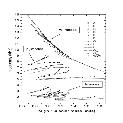
Figure 1: This diagram shows the range of mode-frequencies for twelve different equations of state, as functions of the normalized mass (${\bar{M}}$ of the star.

The few pulsation modes of a neutron star that may be detectable through the associated gravitational waves all have rather high frequencies; typically of the order of several kHz. To illustrate this we show the mode-frequencies for all models considered by Andersson and Kokkotas [Andersson & Kokkotas 1998] as a function of the stellar mass in Figure 1. From this figure we immediately see that a detector must be sensitive to frequencies of the order of 8-12 kHz and above to observe most $w$-modes. Of course, it is also clear that some equations of state yield $w$-modes at somewhat lower frequencies. For example, for massive neutron stars with $M\approx 1.8-2.3M_{\odot}$ (stiff EOS), as have been suggested for low-mass X-ray binaries, the $w$-mode frequency could be as low as 6 kHz (see also recent results for the axial $w$-modes by Benhar et al [Benhar, et al.1999]). The $p$-modes lie mainly in the range 4-8 kHz, while all $f$-modes have frequencies lower than 4 kHz. This means that the mode-signals we consider lie in the regime where an interferometric detector is severely limited by the photon shot noise. For this reason a detection strategy based on resonant detectors (bars, spheres or even networks of small resonant detectors [Frasca & Papa1995]) or laser interferometers operating in dual recycling mode seems the most promising. In fact, the range of mode-frequencies in Fig. 1 should motivate detailed studies of the prospects for construction dedicated ultrahigh frequency detectors. In the following we will compare three different detectors: The initial and advanced LIGO interferometers, for which

$$S_{n}^{1/2}\approx h_{m}\left({f\over\alpha f_{m}}\right)^{3/2}{1\over\sqrt{f}}\ \mbox{Hz}^{-1/2}\;,$$ (13)

with $h_{m}=3.1\times 10^{-22}$, $\alpha=1.4$ and $f_{m}=160$ Hz for the initial configuration, and $h_{m}=1.4\times 10^{-23}$, $\alpha=1.6$ and $f_{m}=68$ Hz respectively, for the advanced configuration [Flanagan & Hughes 1998]. We also consider an “ideal” detector that is tuned to the frequency of the mode and has sensitivity of the order of $S_{n}^{1/2}\approx 10^{-23}$ Hz^-1/2 (this is the sensitivity goal of detectors under construction ). It should be noted that the Advanced LIGO estimates are roughly valid also for spherical detectors such as TIGA, cf. Harry, Stevenson and Paik [Harry et al 1996].

The detectability of the $f$, $p$ and $w$-modes for different detectors can be assessed from (4). The main problem in doing this is the lack of realistic simulations providing information about the level of excitation of various modes in an astrophysical situation. Still, given the frequency and damping rate of a specific mode we can ask what amount of energy must be channeled through the mode in order to be detectable by a given detector. We immediately find that detection of pulsating neutron stars from outside our own galaxy is very unlikely. Let us consider a “typical” stellar model for which the $f$-mode has parameters $f_{f}=2.2$ kHz and $\tau_{f}=0.15$ s. This corresponds to a $1.4M_{\odot}$ neutron star according to the Bethe-Johnson equation of state, cf. Table 3 of Andersson and Kokkotas [Andersson & Kokkotas 1998]. For this example we find that the $f$-mode in the Virgo cluster (at 15 Mpc) must carry an energy equivalent to more than $0.3M_{\odot}c^{2}$ to lead to a signal-to-noise ratio of 10 in our ideal detector. Given that the total energy estimated to be radiated as gravitational waves in a supernova is at the level of $10^{-5}-10^{-6}M_{\odot}c^{2}$, we cannot realistically expect to observe mode-signals from far beyond our own galaxy.

This means that the number of detectable events may be rather low. Certainly, one would not expect to see a supernova in our galaxy more often than once every thirty years, or so. Still, there are a large number of neutron stars in our galaxy, all of which may be be involved in dramatic events (see the introduction for some possibilities) that lead to the excitation of pulsation modes. The energies required to make each mode detectable (with a signal-to-noise ratio of 10) from a source at the center of our galaxy (at 10 kpc) are listed in Table 1. In the table we have used the data for the “typical” stellar model, for which the characteristics of the $f$-mode were given above, $f_{p}=6$ kHz and $\tau_{p}=2$ s, and $f_{w}=11$ kHz and $\tau_{w}=0.02$ ms. This data indicates that, even though the event that excites the modes must be violent, the energy required to make each mode detectable is not at all unrealistic. In fact, the energy levels required for both the $f$- and $p$-modes are such that detection of violent events in the life of a neutron star should be possible, given the Advanced LIGO detectors (or alternatively spheres with the sensitivity proposed for TIGA). On the other hand, detection of $w$-modes with the broad band configuration of LIGO seems unlikely. Detection of these modes, which would correspond to observing a uniquely relativistic phenomenon, requires dedicated high frequency detectors operating in the frequency range above 6 kHz. Still, we believe that the data in Table 1 illustrates that neutron star pulsation modes may well be detectable from within our galaxy, and that the first detection may in fact come as soon as the first generation of LIGO detectors come on line.

Table 1: The estimated energy (in units of $M_{\odot}c^{2}$) required in each mode in order to lead to a detection with signal-to-noise ratio of 10 from a pulsating neutron star at the center of our galaxy (10 kpc).

Detector	$f$-mode	$p$-mode	$w$-mode
Initial LIGO	$4.9\times 10^{-5}$	$4.0\times 10^{-3}$	$6.8\times 10^{-2}$
Adv LIGO	$8.7\times 10^{-7}$	$7.0\times 10^{-5}$	$1.2\times 10^{-3}$
Ideal	$1.4\times 10^{-7}$	$1.3\times 10^{-6}$	$6.4\times 10^{-6}$

3.2 How well can we determine the mode parameters?

Let us now discuss the precision with which we can hope to infer the details of each pulsation mode. After inserting Eq. (3) into formulae (39) and (43) we can compute the relative measurement error in the frequency and the damping time of the waves by some appropriately designed detector. After introducing a convenient parameter ${\cal P}$ according to

$${\cal P}^{-1}=\left({S_{n}^{1/2}\over 10^{-23}{\rm Hz^{-1/2}}}\right)\left({r\over 10{\rm kpc}}\right)\left({E_{\rm gw}\over 10^{-6}M_{\odot}c^{2}}\right)^{-1/2}\;,$$ (14)

we find that the error estimates take the following form

$${\sigma_{f}\over f}\simeq 0.0042\ {\cal P}^{-1}\ {\sqrt{1-2Q^{2}+8Q^{4}\over 4Q^{4}}}\ \left({\tau\over 1{\rm ms}}\right)^{-1},$$ (15)

and

$${\sigma_{\tau}\over\tau}\simeq 0.013\ {\cal P}^{-1}\ {\sqrt{10+8Q^{2}\over Q^{2}}}\ \left({f\over 1{\rm kHz}}\right).$$ (16)

Also, for the time of arrival of the gravitational wave signal we get from (46)

$$\sigma_{T}\simeq 0.0042\ {\cal P}^{-1}{\rm ms}\ .$$ (17)

To illustrate these results we show the relative errors associated with the parameter extraction for the “typical” $1.4M_{\odot}$ stellar model we used in the previous section; see Table 2. We assume that each mode carries the energy required for it to be observed with signal-to-noise ratio of 10, cf. Table 1. (This is a convenient measure since it is independent of the particulars of the detector.)

Table 2: The relative errors in the extraction of the mode parameters assuming a signal-to-noise ratio of 10.

	$\sigma_{f}/f$	$\sigma_{\tau}/\tau$	$\sigma_{T}$ ($10^{-6}$ s)
$f$-mode	$8\times 10^{-5}$	$0.2$	11.3
$p$-mode	$3\times 10^{-6}$	$0.2$	3.8
$w$-mode	$0.1$	$0.3$	1.7

From the sample data in Table 2 one sees clearly that, while an extremely accurate determination of the frequencies of both the $f$- and the $p$-mode is possible, it would be much harder to infer their respective damping rates. It is also clear that an accurate determination of both the $w$-mode frequency and damping will be difficult. To illustrate this result in a different way, we can ask how much energy must be channeled through each mode in order to lead to a 1% relative error in the frequency or the damping rate, respectively. Let us call the corresponding energies $E_{f}$ and $E_{\tau}$. This measure will then be detector dependent, so we list the relevant estimates for the three detector configurations used in Table 1. When the data is viewed in this way, cf. Table 3, we see that an accurate extraction of $w$-mode data will not be possible unless a large amount of energy is released through these modes. Furthermore, one would clearly need a detector that is sensitive at ultrahigh frequencies. In other words, it seems unlikely that we will be able to use the $w$-modes to infer the detailed neutron star parameters as we have previously suggested [Andersson & Kokkotas 1996].

Table 3: The estimated energy (in units of $M_{\odot}c^{2}$) required in each mode in order to lead to a relative error of 1% in the inferred mode-frequency ($E_{f}$) and damping rate ($E_{\tau}$). In cases where no entry is given, the required energy is unrealistically high (typically larger than $M_{\odot}c^{2}$). The distance to the source is assumed to be 10 kpc.

Detector	$f$-mode		$p$-mode		$w$-mode
	$E_{f}$	$E_{\tau}$	$E_{f}$	$E_{\tau}$	$E_{f}$	$E_{\tau}$
LIGO 1	$3.1\times 10^{-9}$	$1.9\times 10^{-2}$	$2.8\times 10^{-10}$	—	—	—
Adv LIGO	$5.5\times 10^{-11}$	$3.5\times 10^{-4}$	$4.9\times 10^{-12}$	$2.8\times 10^{-2}$	$0.17$	—
Ideal	$8.8\times 10^{-12}$	$5.6\times 10^{-5}$	$8.8\times 10^{-14}$	$5\times 10^{-4}$	$9\times 10^{-4}$	$6.1\times 10^{-3}$

4 Revealing the equation of state

In the previous section we discussed issues regarding the detectability of a mode-signal, and the accuracy with which the parameters of the mode could be inferred from noisy gravitational wave data. Let us now assume that we have detected the mode and extracted the relevant parameters. We then naturally want to constrain the supranuclear equation of state by deducing the mass and the radius of the star (or combinations of them). In principle, the mass and the radius can be deduced from any two observables, cf., Table 2 of Andersson and Kokkotas [Andersson & Kokkotas 1998]. In the absence of detector noise, several combinations look promising, but in reality only few combinations are likely to be useful.

Consider the following example: We could in principle deduce the mass and the radius from a detected $f$-mode (assuming that we have extracted both its frequency and damping rate). However, as can be seen from Table 2, the estimated relative error in frequency is about three orders of magnitude smaller than the relative error in damping time. Hence, if these two measurements are to be used to determine the mass and the radius of the pulsating star one must keep in mind that the measurement of frequency is far more accurate than the measurement of damping time. And it is clear that by combining $f_{f}$ with $\tau_{f}$ we will only get accurate estimates for $M$ and $R$ if the energy in the mode is substantial. The same is true for the combination $f_{p}$ and $\tau_{p}$, as well as any combination involving the $w$-mode data. Still, we should not discard the possibility that there will be unique events for which $w$-modes carry the bulk of the energy, as for example the scattering of [Tominanga et al. 1999] or the infall of a smaller mass on neutron stars [Borelli 1997]. In such cases, the strategy proposed by Andersson and Kokkotas [Andersson & Kokkotas 1998] will be useful.

From the data in Tables 1–3, it seems natural to use the $p$-mode in any scheme for deducing the stellar parameters. But, as we have already mentioned, there does not exist a “nice” relation between frequency and stellar parameters for the $p$-mode, that is independent of the equation of state. Still, the strategy that would seem the most promising on the basis of the present results is based on using the frequencies of $f$- and $p$-modes. A possible method is based on the following steps: The first step is to invert the empirical relation for the $f$-mode frequency, Eq. (23), in order to transform the measurement of $f_{f}$ to an estimate of the mean density of the star. Let us define a parameter $x=({\bar{M}}/{\bar{R}}^{3})^{1/2}$, where ${\bar{M}}\equiv M/1.4M_{\odot}$ and ${\bar{R}}\equiv R/10\;{\rm km}$, in order to simplify the notation. Then, once $f_{f}$ has been measured $x$ can be computed from

$$x={{f_{f}({\rm kHz})-0.78}\over 1.63}\;,$$ (18)

with a corresponding relative error

$${\sigma_{x}\over x}=\left[\left({0.97\over\rho}{{\rm 1ms}\over\tau_{f}}{1\over f_{f}-0.78}\right)^{2}\\ +\left({0.01\over f_{f}-0.78}\right)^{2}+0.006^{2}\right]^{1/2}\;,$$ (19)

where $f_{f}$ is expressed in kHz.

The first of the three terms in the square root comes, obviously, from the measurement error of $f_{f}$ (the extra complicating factor, related with the $Q$ of the $f$-mode, that arises there when one tries to express the result with respect to the signal-to-noise, has been simplified to unity since the $Q$ of the $f$-mode is generally a large number). The other two terms arise from dispersion of the data for the various equation of state. For a typical $f$-mode frequency of 2 kHz, and damping time 0.2 s the relative error in $x$ is $\sim 0.01$ (assuming $\rho>6$). Actually, the first term in Eq. (19) is negligible and could be omitted. Therefore

$${\sigma_{x}\over x}\simeq\sqrt{\left({0.01\over f_{f}-0.78}\right)^{2}+0.006^{2}}\;.$$ (20)

Here, we need not worry about the sign of the factor $f_{f}-0.78$; it is always positive since $f_{f}>1.4\;{\rm kHz}$ for every stellar model in the dataset, see Figure 1 here, or Figure 1 of [Andersson & Kokkotas 1998].

Then, by measuring the frequency of the first $p$-mode —which is expected to carry roughly as much energy as the $f$-mode, see Allen et al [Allen, et al. 1998], one could place an error box on a diagram of $f_{p}$ vs. $x$, where all theoretical models for the equation of state are drawn. We illustrate this in Figure 2. This way we can identify the most likely equation of state. Detecting gravitational waves from pulsating neutron stars ensures quite accurate measurements of $f_{f}$ and $f_{p}$, so the error box in Figure 2 is remarkably small. Hence, this method can easily distinguish between the different equations of state in our dataset. In fact, what makes this method so efficient is the fact that different equations of state are described by quite distinct curves in an $f_{p}-x$ diagram.

Figure 2: This diagram shows how the observable frequency of the first $p$-mode scales with the square root of the mean density of a neutron star, (${\bar{M}}/{\bar{R}}^{3}$), according to numerical data for various equations of state.

Finally, we would like to infer the mass and radius of the neutron star. To do this we can use the data in Figure 3, which gives the connection between the $p$-mode frequencies of the different equations of state and the stellar compactness. From this diagram, we can immediately use the detected $f_{p}$ to infer the compactness of the star, once the right equation of state has been identified. Having estimated both the average density and the compactness, it is an elementary calculation to obtain the mass and the radius of the star.

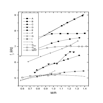
Figure 3: This diagram shows how the observable frequency of the first $p$-mode scales with the compactness of a neutron star, (${\bar{M}}/{\bar{R}}$), according to numerical data for various equations of state.

At this point it is natural to ask the following question: What if the true equation of state is not close to one of the present models? This may well be the case. After all, our understanding of the state of nuclear matter at supranuclear densities still awaits observational testing. Should the equation of state be markedly different from the ones in our sample we will get an error box which does not lie close to any of the equations of state in Figure 2. Should one then want to estimate the stellar parameters, one could construct a sequence of polytropes ($p=K\rho^{\gamma}$, $\gamma=1+1/n$) for various values of $K$ and $n$ (see for example the graphs in [Andersson & Kokkotas 1996]). The appropriate combination of these free parameters will bring the corresponding equation of state within our error box. Then, one could use Figure 3 and read off the “correct” compactness of the star (${\bar{M}}/{\bar{R}}$) and from this compute its radius and mass.

5 Determining the position of the source

As with other kinds of gravitational-wave sources, a network of at least three detectors is needed to pinpoint the location of the source in the sky. The difference in arrival time for the three detectors could be used to determine the position of the source. The higher the accuracy in measuring the time of arrival at each detector, the more precise will be the positioning of the source. Two remote detectors, at a distance $d$ apart from each other will receive the signal with a temporal difference of

$$\Delta T={d\over c}\cos\theta\;,$$ (21)

where $c$ is the speed of light, and $\theta$ is the angle between the line joining the two detectors and the line of sight of the source. Therefore, the accuracy by which this angle can be measured is

$$\Delta\theta={\sqrt{2}\sigma_{T}c\over d\sin\theta}\;.$$ (22)

The $\sqrt{2}$ arises from the measurement errors of the two times of arrival. If one assumes an ‘L’ shaped network of 3 detectors with arm length of $d=10,000$ km, Eqs. (17) and (22) lead to an error box on the sky with angular sides of $1^{\rm o}$, at most (for specific areas of the sky, and large signal-to-noise ratios the angular sizes could be much smaller). This is quite interesting since one could then correlate the detection of gravitational waves with radio- , X-ray or gamma-ray observations directed on that specific corner of the sky.

CONCLUDING REMARKS

In this paper we have extended previous studies of the detectability of gravitational waves from pulsating neutron stars to include the statistical errors associated with an analysis of a weak signal in a noisy data stream. We have shown that the generation of detectors that is presently under construction may well be able to observe such sources from within our own galaxy. Detections from distant galaxies seem unlikely, unless a sizeable amount of energy (of the order of $0.01M_{\odot}c^{2}$) is released through the pulsation modes. This means that we expect the event rate to be rather low. One would certainly not expect to see more than perhaps three neutron stars being born in supernovae per century in our galaxy. Of course, other unique events in a neutron stars life, like starquakes and phase-transitions, may lead to relevant signals. Perhaps the most interesting possibility is the possible association between gravitational waves from pulsation modes and gamma rays from the soft-gamma repeaters (the magnetars). The number of such events is very hard to estimate at the present time. Given the many uncertainties in the available models of all these scenarios, we certainly cannot rule out the possibility of detecting gravitational waves from pulsations in neutron stars.

However, and this is an important point, the chances of detecting pulsating neutron stars would be much enhanced if one could construct dedicated high-frequency gravitational-wave detectors sensitive in the range 5-10 kHz. This provides a serious challenge to experimenters, but that the pay-off of a successful detection of oscillating neutron stars would be great is clear from our present analysis of the inverse problem. We have shown that the oscillation frequencies of the fluid $f$ and $p$ modes can be accurately deduced from detected signals. Other parameters, like the particulars of the gravitational-wave $w$ modes will be much more difficult to infer, unless the signal-to-noise ratio of the detection is unexpectedly large. This means that a previously proposed strategy for deducing the parameters of the star (the mass and the radius) from observations of the $f$ and a $w$-mode is unlikely to be practical. However, we show that an equally powerful strategy can be based on detected $f$ and $p$-modes. Given an observation of $f$ and $p$-mode oscillation frequencies, with the estimated accuracies, we can easily rule out many proposed equations of state. In other words, we have proposed a gravitational-wave “fingerprint analysis” for neutron stars holds a lot of promise, and may help us reveal the true equation of state at supranuclear densities once gravitational waves are observed.

Appendix A EMPIRICAL RELATIONS

In this Appendix we list the empirical relations deduced from data for twelve different realistic equations of star. These relations between the observables (frequency and damping of the modes) and the stellar parameters (mass $M$ and radius $R$) are essentially the same as the ones listed by Andersson and Kokkotas [Andersson & Kokkotas 1998], but here we also include the relevant statistical errors.

We have constructed empirical relations for both the fundamental mode of fluid pulsation (the $f$-mode) and the slowest damped of the gravitational wave $w$-modes. For the $f$-mode, the frequency scales with the mean density of the neutron star according to

$${f_{f}\over 1\;{\rm kHz}}\simeq(0.78\pm 0.01)+(1.63\pm 0.01)\left({{\bar{M}}\over{\bar{R}}^{3}}\right)^{1/2}\;,$$ (23)

while the damping time of the $f$-mode can be described by

$${1{\rm s}\over\tau_{f}}\simeq\left({{\bar{M}}^{3}\over{\bar{R}}^{4}}\right)\left[(22.85\pm 1.51)-(14.65\pm 1.32)\left({{\bar{M}}\over{\bar{R}}}\right)\right]\;,$$ (24)

where ${\bar{M}}\equiv M/1.4M_{\odot}$ and ${\bar{R}}\equiv R/10\;{\rm km}$. The indicated uncertainties are simply the statistical errors that show up if one takes into account all stellar models in the data set, on equal basis. In principle, equations (23) and (24) could be inverted to compute the average density (${\bar{M}}/{\bar{R}}^{3}$) and compactness (${\bar{M}}/{\bar{R}}$) of the star from measured values of $f_{f}$ and $\tau_{f}$. However, this procedure proves unreliable since Eq. (24) is a double-valued function with respect to compactness, and the presence of errors makes it impossible to infer the compactness of the star with reasonable accuracy, even if the characteristics of the waves could be measured with extreme precision.

The $w$-modes are pulsations directly associated with spacetime itself. They have relatively high oscillation frequencies (6-14 kHz for typical neutron stars) and barely excite any fluid motion. They are also rapidly damped, with typical lifetime of fraction of a millisecond. The frequency of the first $w$-mode scales with the stellar compactness as

$${f_{w}\over 1\;{\rm kHz}}\simeq{1\over{\bar{R}}}\left[(20.95\pm 0.33)-(9.17\pm 0.29)\left({{\bar{M}}\over{\bar{R}}}\right)\right]\;,$$ (25)

while the damping rate of the mode is well described by

$${{{\bar{M}}}\over\tau_{w}\mbox{ (ms)}} \simeq (3.90\pm 4.39)+(104.06\pm 8.33)\left({{\bar{M}}\over{\bar{R}}}\right)$$ (26)

$$- (67.28\pm 3.84)\left({{\bar{M}}\over{\bar{R}}}\right)^{2}\ .$$ (27)

Appendix B THE FISHER AND COVARIANCE MATRIX

For a typical mode signal the components of the symmetric Fisher matrix, defined by

$$\Gamma_{ij}\equiv 2\Big{\langle}{\partial h\over\partial\theta_{i}}\mid{\partial h\over\partial\theta_{j}}\Big{\rangle}\;,$$ (28)

where $\theta_{i}=(\epsilon,\eta,\zeta,\xi)$ are

$$\Gamma_{\epsilon\epsilon}={1+24Q^{4}+32Q^{6}\over(1+4Q^{2})^{2}}\rho^{2}\;,$$ (29)

$$\Gamma_{\epsilon\eta}={3-4Q^{2}\over 2(1+4Q^{2})^{2}}\rho^{2}\;,$$ (30)

$$\Gamma_{\epsilon\zeta}=-2Q^{2}\rho^{2}\;,$$ (31)

$$\Gamma_{\epsilon\xi}={1\over 1+4Q^{2}}\rho^{2}\;,$$ (32)

$$\Gamma_{\eta\eta}={3+6Q^{2}+8Q^{4}\over(1+4Q^{2})^{2}}\rho^{2}\;,$$ (33)

$$\Gamma_{\eta\zeta}={1\over 2}\rho^{2}\;,$$ (34)

$$\Gamma_{\eta\xi}={3+4Q^{2}\over 2(1+4Q^{2})}\rho^{2}\;,$$ (35)

$$\Gamma_{\zeta\zeta}=(1+4Q^{2})\rho^{2}\;,$$ (36)

$$\Gamma_{\zeta\xi}=0\;,$$ (37)

$$\Gamma_{\xi\xi}=\rho^{2}\;.$$ (38)

The inverse of the Fisher matrix, $\Sigma_{ij}\equiv\Gamma_{ij}^{-1}$, the so-called covariance matrix, has the following components:

$$\Sigma_{\epsilon\epsilon}={1-2Q^{2}+8Q^{4}\over 2Q^{4}(1+4Q^{2})}{1\over\rho^{2}}\;,$$ (39)

$$\Sigma_{\epsilon\eta}={3-4Q^{2}\over Q^{2}(1+4Q^{2})}{1\over\rho^{2}}\;,$$ (40)

$$\Sigma_{\epsilon\zeta}={-1+4Q^{2}\over 2Q^{2}(1+4Q^{2})}{1\over\rho^{2}}\;,$$ (41)

$$\Sigma_{\epsilon\xi}={-1+Q^{2}\over 2Q^{4}}{1\over\rho^{2}}\;,$$ (42)

$$\Sigma_{\eta\eta}={4(5+4Q^{2})\over(1+4Q^{2})}{1\over\rho^{2}}\;,$$ (43)

$$\Sigma_{\eta\zeta}={-4\over(1+4Q^{2})}{1\over\rho^{2}}\;,$$ (44)

$$\Sigma_{\eta\xi}={-3-2Q^{2}\over Q^{2}}{1\over\rho^{2}}\;,$$ (45)

$$\Sigma_{\zeta\zeta}={2\over(1+4Q^{2})}{1\over\rho^{2}}\;,$$ (46)

$$\Sigma_{\zeta\xi}={1\over 2Q^{2}}{1\over\rho^{2}}\;,$$ (47)

$$\Sigma_{\xi\xi}={(1+2Q^{2})^{2}\over 2Q^{4}}{1\over\rho^{2}}\;.$$ (48)

These relations can be used to estimate the measurement error in the various parameters of the mode-signal; see discussion in the main text.

References

- [Alcock et al 1986] Alcock C., Farhi E., Olinto A. 1986, ApJ, 310, 261
- [Allen, et al. 1998] Allen G., Andersson N., Kokkotas K.D., Schutz B.F, 1998, Phys.Rev.D, 58, 124012
- [Allen, et al. 1999] Allen G., Andersson N, Khanna G, Kokkotas K.D., Laguna P., Pullin J.A., Ruoff J. 1999, Neutron star collisions: The close limit in preparation
- [Andersson 1998] Andersson N. 1998, ApJ, 502, 708
- [Andersson & Kokkotas 1996] Andersson N., Kokkotas K.D., 1996, Phys. Rev. Letters, 77, 4134
- [Andersson & Kokkotas 1998] Andersson N., Kokkotas K.D., 1998, MNRAS,299, 1059
- [Andersson, Kokkotas & Schutz 1999] Andersson N., Kokkotas K.D., Schutz B.F. 1999, ApJ, in press astro-ph/9805225
- [Baumgarte et al 1996] Baumgarte T.W., Janka H-T., Keil W., Shapiro S.L., Teukolsky S.A. 1996, ApJ, 468, 823
- [Benhar, et al.1999] Benhar O., Berti E., Ferrari V., 1999, preprint gr-qc/9901037
- [Blaes 1997] Blaes O., Blandford R., Goldreich P., Madau P., 1989, ApJ 343, 839
- [Borelli 1997] Borelli A., 1997, Nuovo Cimento, B112, 225
- [Duncan 1992] Duncan R.C., 1998 ApJ, 498, L45
- [Duncan & Thompson 1992] Duncan R.C., Thompson C. 1992, ApJ, 392, L9
- [Finn1992] Finn L.S., 1992, Phys. Rev. D, 46, 5236
- [Echeverria1989] Echeverria F., 1989, Phys. Rev. D, 40, 3194
- [Flanagan & Hughes 1998] Flanagan , Hughes S., 1998, Phys. Rev. D, 57, 4235
- [Frasca & Papa1995] Frasca S., Papa M.A., 1995, Int. J.Mod.Phys., 4, 1
- [Friedman & Morsink 1998] Friedman J.L., Morsink S. 1998, ApJ, 502, 714
- [Harry et al 1996] Harry G.M., Stevenson T.R., Paik H.J., 1996, Phys. Rev. D, 54, 2409
- [Kokkotas 1997] Kokkotas K.D. 1997 in Relativistic Gravitation and Gravitational Radiation eds Marck J.-A. and Lasota J.-P. (Cambridge University Press)
- [Kokkotas & Schutz 1986] Kokkotas K.D., Schutz B.F., 1986, G.R.G., 18, 913
- [Kokkotas & Schutz 1992] Kokkotas K.D., Schutz B.F., 1992, MNRAS, 255, 119
- [Kokkotas & Schäfer 1995] Kokkotas K.D., Schäfer G., 1995, MNRAS, 275, 301
- [Lindblom and Detweiler 1983] Lindblom L., Detweiler S., 1983, ApJ Suppl 53, 73
- [Mock & Joss 1997] Mock P.C., Joss P.C., 1998, ApJ 500, 374
- [Schutz 1997] Schutz B.F. 1997 in Detection of gravitational waves in Proceedings of “Astrophysical sources of gravitational radiation” Eds: J.A. Marck and J.P. Lasota (Cambridge Univ. Press 1997)
- [Spruit & Phinney 1998] Spruitt H., Phinney E.S. 1998, Nature, 393, 139
- [Thorne 1987] Thorne K.S., in 300 Years of Gravitation, eds. S. W. Hawking and W. Israel (Cambridge University Press, Cambridge, 1987), p. 330.
- [Tominanga et al. 1999] Tominaga K., Saijo M, Maeda K., 1999, preprint gr-qc/9901040