Data analysis strategies for the detection of gravitational waves in non-Gaussian noise

Abstract

In order to analyze data produced by the kilometer-scale gravitational wave detectors that will begin operation early next century, one needs to develop robust statistical tools capable of extracting weak signals from the detector noise. This noise will likely have non-stationary and non-Gaussian components. To facilitate the construction of robust detection techniques, I present a simple two-component noise model that consists of a background of Gaussian noise as well as stochastic noise bursts. The optimal detection statistic obtained for such a noise model incorporates a natural veto which suppresses spurious events that would be caused by the noise bursts. When two detectors are present, I show that the optimal statistic for the non-Gaussian noise model can be approximated by a simple coincidence detection strategy. For simulated detector noise containing noise bursts, I compare the operating characteristics of (i) a locally optimal detection statistic (which has nearly-optimal behavior for small signal amplitudes) for the non-Gaussian noise model, (ii) a standard coincidence-style detection strategy, and (iii) the optimal statistic for Gaussian noise.

The reliable detection of weak gravitational wave signals from broad-band detector noise from kilometer-scale interferometers such as LIGO [1] and VIRGO [2] is the primary concern in developing gravitational wave data analysis strategies. Because of the weakness of the expected gravitational wave signals, it is critical that the detection strategy should be nearly optimal. However, the detector noise may not be purely stationary and Gaussian, so it is important that the detection strategy also be robust so that detections will be reliable.

Until now, most work on the development of data analysis strategies has been limited to the case of stationary Gaussian noise, though there has been some work [3] on the creation of vetoes that will discriminate between expected gravitational wave signals and non-Gaussian noise bursts. Because the properties of the noise in the LIGO and VIRGO detectors will not be known in advance, it is difficult to assess how well these strategies and vetoes will perform. When real interferometer data from the 40-meter Caltech prototype is used, it is found that additional vetoes are needed to deal with the abundance of false alarms arising from the non-Gaussian noise [4, 5].

In this paper, I present a simple non-Gaussian noise model, consisting of Poisson-distributed noise bursts, that represents a number of potential non-Gaussian noise sources that may be present in future interferometers. This noise model is less naïve than the usual assumptions of Gaussian noise alone, but is simple enough that many analytical results can be obtained. By using this noise model, the robustness of various detection strategies can be assessed. A general introduction to signal detection in non-Gaussian noise can be found in Ref. [6]. The new result in this paper is the use of the non-Gaussian noise model in examining the performance of simple multi-detector search strategies, which will be important for gravitational wave searches.

I will adopt the following notation in this paper. The detector output is a set of $N$ values that are written collectively as a vector ${\mathbf{h}}$ in a $N$-dimensional vector space $V$. This vector can be thought of as having components $h_{j}=({\mathbf{h}},{\mathbf{e}}_{j})$, $j\in[0,N-1]$, which represent a time series of sample measurements made by the detector. Here, ${\mathbf{e}}_{j}$ is the appropriate Cartesian basis on $V$. Alternatively, the vector can be expressed as the set of components $\{\tilde{h}_{2k},\tilde{h}_{2k+1}\}$, $k\in[0,N/2-1]$—the real and imaginary Fourier transform components of $\{h_{j}\}$. These components are given by $\tilde{h}_{j}=({\mathbf{h}},\tilde{{\mathbf{e}}}_{j})$, where $\tilde{{\mathbf{e}}}_{2k}=(2/N)^{1/2}\sum_{j=0}^{N-1}{\mathbf{e}}_{j}\cos(2\pi jk/N)$ and $\tilde{{\mathbf{e}}}_{2k+1}=(2/N)^{1/2}\sum_{j=0}^{N-1}{\mathbf{e}}_{j}\sin(2\pi jk/N)$, $k\in[0,N/2-1]$. Thus, the vectors can be treated in either a time representation or a frequency representation.

A natural inner product of two vectors, ${\mathbf{a}}$ and ${\mathbf{b}}$, in this vector space is defined as $({\mathbf{a}},{\mathbf{Q}}{\mathbf{b}})$. The kernel ${\mathbf{Q}}$ is the inverse of the auto-correlation matrix, ${\mathbf{R}}$, of the Gaussian component, ${\mathbf{n}}_{\text{G}}$, of the detector noise. Thus, ${\mathbf{R}}=\langle{\mathbf{n}}_{\text{G}}\otimes{\mathbf{n}}_{\text{G}}\rangle$, where the angle brackets denote an average over an ensemble of realizations of detector noise. Vector norms are defined in terms of this inner product, i.e., $\|{\mathbf{a}}\|^{2}=({\mathbf{a}},{\mathbf{Q}}{\mathbf{a}})$, as are unit vectors: $\hat{\mathbf{a}}={\mathbf{a}}/\|{\mathbf{a}}\|$.

The detector noise ${\mathbf{n}}$ consists of two components: (i) the Gaussian component ${\mathbf{n}}_{\text{G}}$ (that is always present) and (ii) a possible noise burst component ${\mathbf{n}}_{\text{B}}$ that is present with probability $P_{\text{B}}$. The Gaussian component has the probability distribution $p[{\mathbf{n}}_{\text{G}}]\propto\exp(-\|{\mathbf{n}}_{\text{G}}\|^{2}/2)$. If the burst component is randomly distributed in the vector space $V$ with normalized measure $\hat{D}[{\mathbf{n}}_{\text{B}}]$, then the probability distribution for the noise is

$$p[{\mathbf{n}}]\propto e^{-\|{\mathbf{n}}\|^{2}/2}+\frac{P_{\text{B}}}{1-P_{\text{B}}}\int\hat{D}[{\mathbf{n}}_{\text{B}}]e^{-\|{\mathbf{n}}-{\mathbf{n}}_{\text{B}}\|^{2}/2}.$$ (1)

Suppose that the noise bursts are uniformly-distributed in the vector space $V$ out to a large radius $R$. Such bursts will typically last the entire duration of interest ($N$ samples) and fill the entire frequency band. The noise distribution is approximately

$$p[{\mathbf{n}}]\propto e^{-\|{\mathbf{n}}\|^{2}/2}(1+\epsilon e^{\|{\mathbf{n}}\|^{2}/2})$$ (2)

for $\|{\mathbf{n}}\|<R$, where $\epsilon\simeq 2^{N/2}\Gamma(N/2+1)R^{-N}P_{\text{B}}/(1-P_{\text{B}})$ for large $R$.

An alternative derivation of Eq. (2) is the following. Suppose the noise burst is simply an additional transient source of Gaussian noise. Then Eq. (2) can be written as

$$p[{\mathbf{n}}]\propto e^{-({\mathbf{n}},{\mathbf{Q}}{\mathbf{n}})/2}(1+\varepsilon e^{({\mathbf{n}},[{\mathbf{Q}}-{\mathbf{Q}}^{\prime}]{\mathbf{n}})/2}),$$ (3)

where $\varepsilon=(\det|{\mathbf{R}}|/\det|{\mathbf{R}}^{\prime}|)^{N/2}P_{\text{B}}/(1-P_{\text{B}})$, ${\mathbf{R}}^{\prime}$ is the auto-correlation matrix for both ambient and the burst components of Gaussian noise together, and the matrix ${\mathbf{Q}}^{\prime}$ is the inverse of ${\mathbf{R}}^{\prime}$. If the typical noise burst is much louder than the ambient Gaussian noise, then ${\mathbf{Q}}-{\mathbf{Q}}^{\prime}\approx{\mathbf{Q}}$. Therefore, in the case of loud Gaussian noise bursts, Eq. (3) has the same form as Eq. (2).

The likelihood ratio can now be computed for the two alternative hypotheses: that the output ${\mathbf{h}}={\mathbf{n}}$ is noise alone ($H_{0}$), or that the output ${\mathbf{h}}=A\hat{\mathbf{u}}+{\mathbf{n}}$ is a signal $A\hat{\mathbf{u}}$ of amplitude $A$ embedded in noise ($H_{1}$). The likelihood ratio $\Lambda(A)=p[{\mathbf{h}}\mid H_{1}]/p[{\mathbf{h}}\mid H_{0}]$ is the ratio of the posterior probability of obtaining the observed output ${\mathbf{h}}$ given hypothesis $H_{1}$ to the posterior probability of obtaining ${\mathbf{h}}$ given hypothesis $H_{0}$. One then finds that the likelihood ratio is

$$\Lambda(A)=\frac{\Lambda_{\text{G}}(A)+\alpha}{1+\alpha}$$ (4)

where

$$\Lambda_{\text{G}}(A)=e^{A(\hat{\mathbf{u}},{\mathbf{Q}}{\mathbf{h}})-A^{2}/2}$$ (5)

and

$$\alpha=\epsilon e^{\|{\mathbf{h}}\|^{2}/2}.$$ (6)

The quantity $\Lambda_{\text{G}}(A)$ is the likelihood ratio one would obtain if only the Gaussian noise component were present; it is a monotonically increasing function of the matched filter $(\hat{\mathbf{u}},{\mathbf{Q}}{\mathbf{h}})$. When a non-Gaussian noise burst component can occur, the likelihood ratio depends on an additional measured quantity: the magnitude of the output vector, $\|{\mathbf{h}}\|$. In addition to these functions of the detector output, the likelihood ratio also depends on the expected amplitude $A$ of the signal and the proportionality factor $\epsilon$, which encapsulates the probability of a noise burst and the maximum possible amplitude $R$ of the burst.

The quantity $\alpha$ plays a central role in the modified likelihood ratio of Eq. (4): it acts as a detector of noise bursts, and vetoes events that are more likely due to the burst. The logarithm of $\alpha$ is proportional to the amount of power in the detector output. For Gaussian noise alone, the expected value of the power is $\langle\|{\mathbf{n}}_{\text{G}}\|^{2}\rangle=N$, and thus $\langle\ln\alpha\rangle\sim\ln P_{\text{B}}-\frac{1}{2}N\ln(R^{2}/N)$ for large $N$. Thus, for $R^{2}>N$ (as was assumed above), the value of $\alpha$ will be small. However, when a noise burst is present, the value of $\ln\alpha$ is increased by a typical amount $\sim\frac{1}{2}R^{2}$, so $\alpha$ will typically become large. In fact, $\alpha$ is the excess-power statistic for detection of arbitrary noise bursts [8, 9]. For small values of $\alpha$, the likelihood ratio approaches the usual Gaussian noise likelihood ratio. However, for large values of $\alpha$, the likelihood ratio approaches unity.

The likelihood ratio is a function of the detector output via the two quantities $x=(\hat{\mathbf{u}},{\mathbf{Q}}{\mathbf{h}})=\|{\mathbf{h}}\|\cos\theta$ and $\|{\mathbf{h}}\|$. The likelihood ratio also depends on the expected signal amplitude $A$ and the factor $\epsilon$. Thus, the likelihood ratio is

$$\Lambda(A)=\frac{e^{Ax-A^{2}/2}+\epsilon e^{(x\sec\theta)^{2}/2}}{1+\epsilon e^{(x\sec\theta)^{2}/2}}.$$ (7)

Figure 1 shows the likelihood ratios as functions of the matched filter statistic $x$ and the angle $\theta$ for a given value of $\epsilon$ and $A$. Notice that the likelihood ratio is attenuated when the magnitude of the output, ${\mathbf{h}}$, is much larger than the largest expected signal; this attenuation occurs at smaller signal-to-noise ratios for smaller absolute values of the direction cosine $\cos\theta$.

Because of the non-trivial dependence of the likelihood ratio on the expected signal amplitude, the optimal statistic for signals of some amplitude $A$ will not be the same statistic as the optimal statistic for a different amplitude $A^{\prime}$. This situation is unlike the case of purely Gaussian noise, for which the likelihood ratio grows monotonically with the matched filter output, regardless of the expected signal amplitude. Because the amplitude of a signal will not typically be known in advance, it is useful to consider a locally optimal statistic [6], which provides the optimal performance in the limit of small amplitude signals. The rationale behind such a choice is that large amplitude signals pose no challenge for detection, so any reasonable statistic will suffice for them. The locally optimal statistic, which is defined as $\lambda=d\ln\Lambda/dA|_{A=0}=(\hat{\mathbf{u}},-\mathchoice{{\hbox{\boldmath$\displaystyle\nabla$}}}{{\hbox{\boldmath$\textstyle\nabla$}}}{{\hbox{\boldmath$\scriptstyle\nabla$}}}{{\hbox{\boldmath$\scriptscriptstyle\nabla$}}}\ln p[{\mathbf{h}}])$, is given by

$$\lambda=\frac{x}{1+\epsilon e^{(x\sec\theta)^{2}/2}},$$ (8)

where $x=(\hat{\mathbf{u}},{\mathbf{Q}}{\mathbf{h}})$ is the matched filter. Notice that the locally optimal statistic also incorporates a veto based on the value of $\alpha=\epsilon\exp[(x\sec\theta)^{2}/2]$. The locally optimal statistic grows approximately linearly for $x<(-2\ln\epsilon)^{1/2}\cos\theta$, at which point it is effectively cut off. This is the same general behavior as was seen before for the likelihood ratio $\Lambda(A)$, but there is no longer any scaling with a prior amplitude.

Another approach is to use a prior distribution $f(A)$ for the amplitude, if such a distribution is known, to construct an integrated likelihood ratio $\Lambda=\int\Lambda(A)f(A)dA$; this integrated likelihood ratio would then be the optimal statistic for detection of all potential signals. Even if the prior distribution is not known, it is possible to obtain an approximate likelihood ratio if $f(A)$ is a slowly-varying function. One can show that $\Lambda_{\text{G}}=\int\Lambda_{\text{G}}(A)f(A)dA\approx f(x)\exp(x^{2}/2)$. A further approximation neglects the slowly-varying function entirely; one then obtains $\Lambda_{\text{G}}\approx\exp(x^{2}/2)$. Thus,

$$\Lambda\approx\frac{e^{x^{2}/2}+\epsilon e^{(x\sec\theta)^{2}/2}}{1+\epsilon e^{(x\sec\theta)^{2}/2}}.$$ (9)

It is important to generalize the above analysis to the case in which there are multiple detectors. Such a situation is deemed to be essential for gravitational wave searches since a coincident detection is an important corroboration that a signal is of an astronomical origin rather than internal to the detector. As a simple model, consider two gravitational wave detectors with identical but independent noise (including possible noise bursts) that also have the same response to gravitational wave signals. If the noise was purely Gaussian, the likelihood ratio for the two detectors together would be $\Lambda_{\text{G}}^{\text{AB}}=\Lambda_{\text{G}}^{\text{A}}\times\Lambda_{\text{G}}^{\text{B}}$, i.e., the product of the likelihood ratios for Gaussian noise in each separate detector. The resulting likelihood ratio is thus an monotonically increasing function of the sum of the matched filter values in each detector: $\ln\Lambda_{\text{G}}^{\text{AB}}\sim x^{\text{A}}+x^{\text{B}}$ where $x^{\text{A}}=(\hat{\mathbf{u}},{\mathbf{Q}}^{\text{A}}{\mathbf{h}}^{\text{A}})$ is the signal-to-noise ratio in the first detector (A) and $x^{\text{B}}=(\hat{\mathbf{u}},{\mathbf{Q}}^{\text{B}}{\mathbf{h}}^{\text{B}})$ is the signal-to-noise ratio in the second detector (B). If the likelihood ratios are integrated over a slowly-varying prior distribution of possible signal amplitudes, then one finds $\ln\Lambda_{\text{G}}^{\text{AB}}\sim(x^{\text{A}}+x^{\text{B}})^{2}$, which also depends on the sum of the two detectors’ matched filter values. (In this case, it is important to integrate over the distribution of amplitudes after multiplying the two detector’s likelihood ratios together since the same signal amplitude should be present in each detector.) Thus, one would decide that a signal was present if the sum of the matched filter values in the two detectors exceeded some threshold. An alternative strategy would decide that a signal was present only if each of the matched filter values exceeded some threshold, i.e., one thresholds on the quantity $\min(x^{\text{A}},x^{\text{B}})$ rather than on $x^{\text{A}}+x^{\text{B}}$.

Suppose the likelihood ratios for both detectors, $\Lambda^{\text{A}}(x^{\text{A}},\theta^{\text{A}})$ and $\Lambda^{\text{B}}(x^{\text{B}},\theta^{\text{B}})$, are given by Eq. (7). Then, the likelihood ratio for the combined detector is given by the product of $\Lambda^{\text{A}}$ and $\Lambda^{\text{B}}$. Figure 2 shows a plot of contours of constant likelihood ratio as a function of the two measured signal-to-noise ratios for $\theta^{\text{A}}=\theta^{\text{B}}=0$ and $\theta^{\text{A}}=0$, $\theta^{\text{B}}=\pi/6$. At low signal-to-noise ratios, the contours are approximately lines of constant $x^{\text{A}}+x^{\text{B}}$—in this regime, the likelihood ratio behaves like the Gaussian likelihood ratio. However, for large values of either $x^{\text{A}}$ or $x^{\text{B}}$, the contours are approximately lines of constant $\min(x^{\text{A}},x^{\text{B}})$.

The locally optimal two-detector statistic is $\lambda^{\text{AB}}=\lambda^{\text{A}}+\lambda^{\text{B}}$, where $\lambda^{\text{A}}$ and $\lambda^{\text{B}}$ both have the form of Eq. (8). This statistic also depends on $x^{\text{A}}$, $x^{\text{B}}$, $\theta^{\text{A}}$, and $\theta^{\text{B}}$. As before, the contours of constant $\lambda^{\text{AB}}$ for fixed $\theta^{\text{A}}$ and $\theta^{\text{B}}$ are lines of constant $x^{\text{A}}+x^{\text{B}}$ for low signal-to-noise ratios but are lines of constant $\min(x^{\text{A}},x^{\text{B}})$ if the signal-to-noise ratio in one of the detectors is large.

These results somewhat justify the use of the minimum statistic $\min(x^{\text{A}},x^{\text{B}})$ when there are two detectors with independent noise operating. When one of the signal-to-noise ratios is large but the other is moderate, the minimum statistic will give approximately the same value as the locally optimal statistic. In this case, the effect of the $\alpha$-based veto in the locally optimal statistic is mimicked in the minimum statistic. The locally optimal statistic is better able to deal with the case when there are noise bursts present in both detectors, but this case occurs with probability $P_{\text{B}}^{2}$, so it should be extremely rare. Moreover, the minimum statistic is less powerful than the locally optimal statistic for small signal-to-noise ratios in both detectors. In this case, the locally optimal statistic is approximately $x^{\text{A}}+x^{\text{B}}$, which is the same as the optimal statistic for Gaussian noise. However, the optimal statistic for Gaussian noise may be unsuitable for the noise model I have considered because the false alarm probability cannot be reduced below $\sim P_{\text{B}}$ for reasonable thresholds. (The minimum statistic suffers the same problem but around the much lower probability $P_{\text{B}}^{2}$.)

To see the relative performance of these statistics, it is useful to consider the operational characteristics of the tests. For some fixed false alarm probability $Q_{0}$, the operational characteristic is the detection probability $Q_{1}$ as a function of signal amplitude. I have computed these curves using Monte Carlo techniques. The noise model I used corresponds to that of Eq. (2) with burst probability $P_{\text{B}}=1\%$ and maximum burst amplitude $R=25$. I fixed the false alarm probability to $Q_{0}=10^{-3}$ and I examined a vector space dimension of $N=4$. Figure 3 shows the relative performances of the three statistics in terms of the detection probability as a function of signal amplitude. One sees that the locally optimal statistic performs the best for small amplitude signals (as expected), but that it has poor performance for large amplitude signals. This is because the large amplitude deviations are interpreted as noise bursts and are suppressed. (If the locally optimal statistic were used in a real search, these large events would not be rejected outright but would rather be subjected to further scrutiny; thus the attenuation of the locally optimal statistic for large signal amplitudes is somewhat misleading.) The sum of the signal-to-noise ratio, which is optimal statistic for Gaussian noise, is seen to have poor performance. The reason is that because the false alarm probability is much smaller than the burst probability, the threshold required for this statistic becomes unreasonably large. However, since the false alarm probability is much higher than the burst probability squared, the minimum statistic performs reasonably well for both small and large amplitude signals.

The conclusion that can be drawn from this analysis is that search strategies based on a Gaussian noise model can be significantly improved by considering a more realistic non-Gaussian noise model, which may contain noise bursts that occur relatively frequently. If a method can be devised to detect these noise bursts and veto data that contains a noise burst, then the use of such a veto effectively reproduces the locally optimal strategy for the noise model containing bursts. However, the necessary veto may not be easily found since it may not be possible to determine the non-Gaussian properties of the detector noise to sufficient accuracy. A viable alternative when two detectors are operating is to use a coincidence strategy of detection. Since the minimum statistic used in the coincidence strategy is a robust statistic, one would expect that it should have good performance for any realistic noise model.

I would like to thank Bruce Allen, Patrick Brady, Éanna Flanagan, and Kip Thorne for their many useful comments on this paper. This work was supported by the National Science Foundation grant PHY-9424337.

FIG. 1.: Likelihood ratio as a function of the matched filter signal-to-noise ratio $x=(\hat{\mathbf{u}},{\mathbf{Q}}{\mathbf{h}})$ and the direction cosine $\cos\theta=(\hat{\mathbf{u}},{\mathbf{Q}}\hat{\mathbf{h}})$. The model signal and noise burst both lie in an $N=4$ dimensional vector space $V$. The model signal has an amplitude $A=5$. Noise bursts occur with a probability $P_{\text{B}}=1\%$; the possible burst vectors are uniformly distributed in $V$ out to a maximum radius $R=25$. The thin solid line is the likelihood ratio if no noise bursts were present ($\epsilon=0$), while the thick dotted lines are plots of Eq. (7) with $\epsilon=2\times 10^{-7}$ (corresponding to the above parameters).

FIG. 2.: Contours of constant likelihood ratio for two detectors, A and B, measuring signal-to-noise ratios $x^{\text{A}}$ and $x^{\text{B}}$. The combined likelihood ratio is the product of individual detector likelihood ratios, which are of the form of Eq. 7 with $A=5$ and $\epsilon=2\times 10^{-7}$. The top plot represents the case when $\theta^{\text{A}}=\theta^{\text{B}}=0$ while the bottom plot represents the case when $\theta^{\text{A}}=0$ and $\theta^{\text{B}}=\pi/6$. Notice that the right side (beyond $x^{\text{B}}\simeq 5$) of the bottom plot is compressed compared to the top plot, while the left hand side of the two plots are roughly the same.

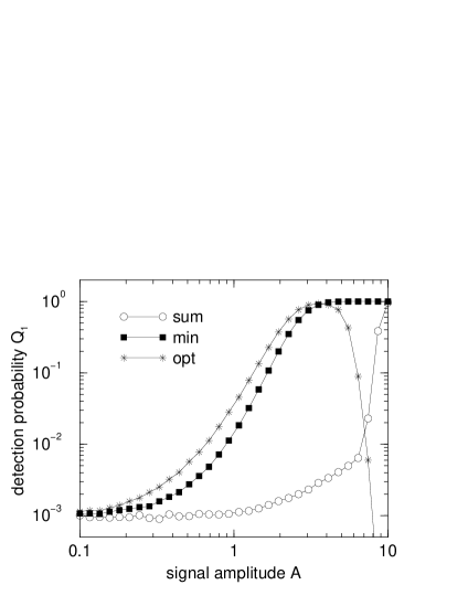
FIG. 3.: The operation characteristics, which express the detection probability $Q_{1}$ as a function of signal amplitude $A$ for fixed false alarm probability $Q_{0}=10^{-3}$ for three multi-detector statistics. The “sum” statistic adds the signal-to-noise ratios of the two detectors; this is the optimal statistic for purely Gaussian noise. The “min” statistic is simply the minimum of the two signal-to-noise ratios. The “opt” statistic is the locally optimal statistic for the noise model. The noise model has a burst probability of $P_{\text{B}}=1\%$, a maximum burst amplitude of $R=25$, and a vector space dimension $N=4$.

REFERENCES

- [1] A. Abramovici et al., Science 256, 325 (1992).
- [2] B. Caron et al., Class. Quantum Grav. 14, 1461 (1997); C. Bradaschia et al., Nucl. Instrum. Methods A 289, 518 (1990).
- [3] B. Allen, GRASP: a data analysis package for gravitational wave detection (http://www.lsc-group.phys.uwm.edu, 1998).
- [4] B. Allen et al., (in preparation).
- [5] J. D. E. Creighton, (in preparation).
- [6] S. A. Kassam, Signal Detection in Non-Gaussian Noise (Springer-Verlag, New York, 1988).
- [7] L. A. Wainstein and V. D. Zubakov, Extraction of signals from noise (Prentice-Hall, London, 1962).
- [8] É. É. Flanagan and S. A. Hughes, Phys. Rev. D 57, 4535 (1998); 57, 4566 (1998).
- [9] W. G. Anderson, P. R. Brady, J. D. E. Creighton, and É. É. Flanagan, (in preparation).
- [10] L. S. Finn, (in preparation).