Adaptive Finite Elements and Colliding Black Holes

Abstract

According to the theory of general relativity, the relative acceleration of masses generates gravitational radiation. Although gravitational radiation has not yet been detected, it is believed that extremely violent cosmic events, such as the collision of black holes, should generate gravity waves of sufficient amplitude to detect on earth. The massive Laser Interferometer Gravitational-wave Observatory, or LIGO, is now being constructed to detect gravity waves. Consequently there is great interest in the computer simulation of black hole collisions and similar events, based on the numerical solution of the Einstein field equations. In this note we introduce the scientific, mathematical, and computational problems and discuss the development of a computer code to solve the initial data problem for colliding black holes, a nonlinear elliptic boundary value problem posed in an unbounded three dimensional domain which is a key step in solving the full field equations. The code is based on finite elements, adaptive meshes, and a multigrid solution process. Here we will particularly emphasize the mathematical and algorithmic issues arising in the generation of adaptive tetrahedral meshes.

1 Introduction

In Einstein’s theory of general relativity space-time is represented as a four-dimensional semi-Riemannian manifold. The geodesics of this manifold are the paths of freely falling particles and gravity is the manifestation of the curvature of space-time. A system of nonlinear partial differential equations, the Einstein field equations, specify the relationship between the curvature of the space-time manifold and the mass-energy it contains. A consequence of the theory is that when a mass accelerates it gives rise to tiny ripples in the fabric of space time, called gravity waves. More precisely, if a mass accelerates in distant space, gravity waves will propogate from the mass at the speed of light. They will be detectable as slight variations in the lengths of objects at the point of observation, these variations modulating with time and differing according to the direction in which the lengths are measured. Consequently gravity waves may be regarded as signals which transmit information about the dynamics of distant space-time. As a window to the universe not confined to the electromagnetic spectrum gravity waves have immense potential as conveyors of information about the universe, and the creation of an effective gravity wave detector could be an event whose significance to astrophysics is as great as the invention of the optical telescope or radio telescope.

Because of their tiny amplitude, gravity waves have eluded detection until now. Even very massive cosmological events, such as the spiralling collision of neutron stars or black holes of several solar masses at a distance from earth of up to about 100 million light years (on the order of 1,000 Milky Way diameters), will cause only the slightest distance changes here at earth—on the order of one part in $10^{22}$. Although the measurement of such tiny distance changes has not been feasible heretofore, many physicists believe that technology has reached a point where gravity wave detection is possible, and several large projects to construct gravitational wave observatories are now underway. The largest of these is the LIGO project (Laser Interferometer Gravitational-wave Observatory), presently under construction in Hanford, Washington and Livingston Parish, Louisiana. Each of the two LIGO installations, like observatories being built in Italy, Germany, Japan, and Australia, is essentially a Michelson interferometer, consisting of a long evacuated L-shaped tube. A laser beam is split at the vertex of the tube and bounced back and forth many times between mirrors at the vertex and at the end of each of the legs. Phase differences can then be detected to measure changes in lengths of the legs. In the case of LIGO, each leg will be about 1.25 meters in diameter and 4 kilometers long, and it will be necessary to measure distance changes of about $10^{-18}$ meters. (For comparison, the diameter of a hydrogen atom is about $10^{-10}$ meters.)

In addition to the immense technological hurdles in the construction of LIGO (e.g., the very sophisticated optics required, the need for a large and near perfect vacuum, and the suppression of a variety of sources of noise), the project also raises an extremely challenging problem of scientific computation. Given a detected gravitational waveform, we must determine the cosmological events that could have given rise to it. The key step in solving this inverse problem is, as usual, the solution of the forward problem, which in this case is the numerical solution of the Einstein field equations. Because they are expected to be a major source of gravitational radiation, and also because they entail some useful simplifications, many researchers are presently focussing on the case of binary black hole collisions. The data of the problem then consists of the initial masses, positions, and linear and angular momenta of the black holes, and the goal is to obtain the far field waveforms generated via numerical solution of the Einstein equations.

The full simulation of the spiralling coalesence of two black holes is being actively pursued, but is, at present not effectively achievable. In the next section we describe the derivation of an elliptic boundary value problem called the binary black hole initial data problem, which is an important part of the full problem. In Section 3 we describe the design principles of a code we have written to solve the binary black hole initial data problem and other elliptic boundary value problems in three-dimensional space. The following two sections describe and validate algorithms used in connection with mesh refinement in the code. Finally, we present numerical results. Much of this material appeared in the thesis of the second author [11]. Proofs of two of the theorems, which will not be repeated here, can be found in [1].

2 The Einstein Equations and the Initial Data Problem

In this section we briefly describe the derivation of the elliptic boundary value problem for the black hole initial data problem. For details we refer to [4, 5, 6, 8, 15]. We represent space-time, or a portion of it, by a semi-Riemannian 4-manifold $M$ parametrized by coordinates $x_{\alpha}$, $\alpha=0,1,2,3$. (Greek indices will in general range from $0$ to $3$.) Let $\boldsymbol{g}$ denote the metric tensor with covariant components $g_{\alpha\beta}$ and contravariant components $g^{\alpha\beta}$ (so these two $4\times 4$ symmetric matrices are inverse to one another). The Christoffel connections are defined as

$$\Gamma^{\gamma}_{\alpha\beta}=g^{\gamma\delta}\left(\frac{\partial g_{\delta\alpha}}{\partial x_{\beta}}+\frac{\partial g_{\delta\beta}}{\partial x_{\alpha}}-\frac{\partial g_{\alpha\beta}}{\partial x_{\delta}}\right)$$

(where we use the Einstein’s convention of summation over repeated indices). The Ricci curvature tensor is then

$$R_{\alpha\beta}:=\frac{\partial\Gamma^{\gamma}_{\alpha\beta}}{\partial x^{\gamma}}-\frac{\partial\Gamma^{\gamma}_{\alpha\gamma}}{\partial x^{\beta}}+\Gamma^{\gamma}_{m\gamma}\Gamma^{m}_{\alpha\beta}-\Gamma^{\gamma}_{m\beta}\Gamma^{m}_{\alpha\gamma},$$

and the Einstein tensor may be obtained simply from the Ricci tensor:

$$G_{\alpha\beta}=R_{\alpha\beta}-\frac{1}{2}g^{\gamma\delta}R_{\gamma\delta}g_{\alpha\beta}.$$

Finally, the Einstein equations may be written

$$G_{\alpha\beta}=8\pi T_{\alpha\beta},$$

where the stress-energy tensor $\boldsymbol{T}$ is a given forcing function. In particular, in the case of a vacuum—which is sufficient for the case of black holes, since we only compute outside the holes—the Einstein equations assert the vanishing of the Einstein, and hence Ricci, tensor.

The Einstein equations form a system of 10 second order quasilinear partial differential equations for the 10 components $g_{\alpha\beta}$ of the metric tensor in the 4 independent variables $x_{\alpha}$. (Expanded out, each equation involves over 1,000 terms!) However, the equations are not independent, since the Bianchi identity implies that $\nabla^{\alpha}G_{\alpha\beta}=0$, no matter what the metric $\boldsymbol{g}$. Hence the Einstein system really only asserts six independent equations. Correspondingly there is a non-uniqueness of solutions (gauge freedom) which essentially allows for the arbitrary specification of four of the metric components.

We now describe the Arnowitt–Deser–Misner $3+1$ approach to the solution of the Einstein equations. The metric tensor has signature $(-,+,+,+)$, and we assume that coordinates are chosen so that the variable $t=x_{0}$ is timelike, and that the remaining variables $x_{i}$ (Latin indices range from 1 to 3) are spacelike. We shall refer to the variable $t$ as time and to the $x_{i}$ as spatial variables. The manifold $M$ is then foliated by the spacelike hypersurfaces $\Sigma_{t}$ given by $t=\text{constant}$. The metric $\boldsymbol{g}$ induces a Riemannian metric on each hypersurfaces, which we denote by $\boldsymbol{\gamma}$. Using the restrictions of the functions $x_{i}$, $i=1,2,3$, as coordinates, the covariant components $\gamma_{ij}$ are equal to $g_{ij}$. The complete four dimensional metric $\boldsymbol{g}$ can then be reconstructed from $\boldsymbol{\gamma}$ together with the lapse $\beta_{i}=g_{0i}$ and the shift $\alpha=\sqrt{g^{ij}\beta_{i}\beta_{j}-g_{00}}$. In view of the gauge freedom, we may determine the lapse and shift in any convenient way (just how this is to be done is currently an area of intense investigation). Next we separate the Einstein equations into two separate systems of equations. If we multiply the equations by the normal to the hypersurface $\Sigma_{t}$ we obtain the constraint equations, a system of four equations. The remaining six equations, which arise by multiplying by the tangential directions, are referred to as the evolution equations. These names arise because the constraint equations do not involve second derivatives with respect to $t$. Thus they form a purely spatial system of four second order differential equations in the 12 dependent variables $\gamma_{ij}$ and $\partial\gamma_{ij}/\partial t$ posed on each of the foliating manifolds $\Sigma_{t}$. More geometrically significant dependent variables are obtained by using the components of the extrinsic curvature tensor

$$K_{ij}=-\frac{1}{2\alpha}(\frac{\partial\gamma_{ij}}{\partial t}-\nabla_{j}\beta_{i}-\nabla_{i}\beta_{j})$$

instead of $\partial\gamma_{ij}/\partial t$, and this is usually done. The problem of determining a solution $\gamma_{ij}$, $K_{ij}$ on $\Sigma_{0}$ to the constraint equations is known as the initial data problem. Once a solution to the initial data problem is found, the evolution equations are a system of differential equations, second order in space and time, which can be used to determine $\gamma_{ij}$ for $t>0$. The constraint equations may or may not be imposed at positive times. It can be shown that if they are satisfied at the initial time and the evolution equations are satisfied exactly, then they are satisfied at all times.

The initial data problem is highly underdetermined, and there are many possible solutions. One of the simplest approaches of physical relevance to binary black holes procedes from the assumptions

• The spatial metric is conformally equivalent to a flat metric, i.e., $\gamma_{ij}=\psi^{4}\delta_{ij}$ for some function $\psi:\Sigma_{0}\to\mathbb{R}$ to be determined.

• The manifold $\Sigma_{0}$ is maximally embedded, i.e., the trace of $\boldsymbol{K}$ vanishes.

(This is a special case of the method of conformal imaging of J. York [14].) Under these assumptions three of the four constraint equations (the momentum constraints) are linear and decoupled from the fourth equation, and solutions to them can be determined analytically. The remaining equation (the Hamiltonian constraint) takes the form

$$\Delta\psi+H(x)\psi^{-7}=0,$$ (2.1)

where $H(x)$ depends on the solution to the momentum contraint equations and encodes the positions, masses, and linear and angular momenta of the black holes. To obtain initial data for binary blackhole collisions we wish to solve this equation on $\mathbb{R}^{3}\setminus(B_{1}\cup B_{2})$ where the $B_{i}$ are disjoint balls (their boundaries are the apparent horizons of the holes). The equations are subject to Robin boundary conditions

$$\frac{\partial\psi}{\partial r_{i}}+\frac{1}{2r_{i}}\psi=0$$ (2.2)

on the hole boundaries (the apparent horizons of the blackholes), and the condition $\lim_{|x|\to\infty}\psi(x)=1$ at infinity (so that the metric is asymptotic to the flat metric far from the holes). For numerical purposes the latter condition is usually replaced by an artificial boundary condition like

$$\frac{\partial\psi}{\partial r}+\frac{1}{r}(\psi-1)=0$$ (2.3)

on the boundary of a ball $B_{0}$ about the origin containing the holes well within its interior. (Equation (2.3) can be derived by a multipole expansion; cf. [5].)

3 A Code for the Black Hole Initial Data Problem

We thus wish to solve the semilinear boundary value problem consisting of the PDE (2.1) on $B_{0}\setminus(B_{1}\cup B_{2})$, together with the boundary condition (2.2) on $\partial B_{i}$, $i=1$, $2$, and the artificial boundary condition (2.3) on $\partial B_{0}$. In a typical computation the hole radii are of the same general magnitude, as is the distance of their centers from the origin, while the radius of the containing sphere is taken to be two to four orders of magnitude larger. We have designed a code to solve this problem based on the following design principles:

• Because of the nontrivial geometry we use finite elements.

• Since the solution varies significantly over only a small portion of the domain, in the immediate vicinity of the holes, the mesh is refined adaptively.

• We reduce the nonlinear systems of equations to linear problems with Newton’s method.

• We solve the resulting large systems of linear equations using multigrid techniques based on the sequence of adaptively generated meshes.

The gross structure of a code based on these principles is shown in Figure 3.1. (The requirement of conformity in steps 1 and 2(d) means that every nonempty intersection of two distinct tetrahedra must be either a common face, a common edge, or a common vertex.)

1. Begin with an initial coarse conforming tetrahedral mesh matching the geometry and some initial approximation of the solution on that mesh. 2. Do until a sufficiently accurate solution is found: (a) On the current mesh discretize the problem using piecewise linear finite elements. (b) Do until the approximation on the current mesh is sufficiently close to stationary: i. Linearize the finite element problem about the current approximation on the current mesh. ii. Solve the linearized problem using full multigrid to generate the next approximation: Beginning with the coarse mesh solution, interpolate the solution to the next finer mesh and update it by smoothing on the finer mesh and residual correction on the coarser mesh. Continue this process recursively to generate the solution of the linear problem on the current mesh. (c) Assign error indicators to the elements of the current mesh. (d) Refine the mesh as indicated. Refine further to restore conformity thus obtaining the next finer mesh. (e) Use the current solution on the old mesh as the initial approximate solution on the new mesh.

Figure 3.1: Gross structure of the code.

The development of a code along these lines involves many issues. We will discuss two of them here:

• How to refine a tetrahedron, ensuring that its descendants are nicely shaped tetrahedra, even after many generations of refinement?

• How to bring a refined mesh into conformity without over-refining?

4 Tetrahedral Refinement

The two most natural ways to partition a tetrahedron into subtetrahedra are bisection (by placing a new vertex on some particular edge, and connecting it to the existing vertices opposite that edge), and octasection (cutting off each corner by placing a new face through the midpoint of the edges emanating from the corner, and then dividing the remaining octahedron into four tetrahedra). See Figure 4.1. The use of octasection requires a great many intermediate partition strategies if a conforming adaptive mesh is to be maintained (see [3]). However a conforming adaptive refinement can be attained using only bisection. Moreover, since one step of bisection reduces the element volume by a factor of two rather than eight for octasection, it can produce element sizes closer to the optimal ones. Thus we have chosen to base our code exclusively on bisection.

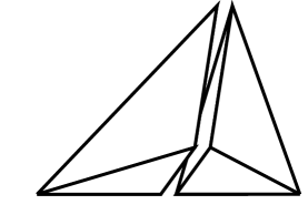
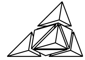
Figure 4.1: Bisection and octasection.

Every time we bisect a tetrahedron we must specify a particular edge, called the refinement edge, on which the new vertex will be placed. (We always place the new vertex at the midpoint of the refinement edge.) Careful selection of the refinement edge is essential if the tetrahedra shapes are not to degenerate after repeated bisections. For bisection of triangular meshes in two dimensions, there are two commonly used algorithms for selection of the bisection edge of a triangle. One approach is to always select the longest edge of the triangle. Rivara [12] has proven that longest-edge bisection can be applied repeatedly without degeneration of element shape. The second approach in two dimensions is opposite-edge bisection. In this approach any edge (e.g., the longest) can be selected for the refinement edge of triangles in the initial mesh, but as new triangles are created by bisection, they are always assigned the edge opposite the newly added vertex as the refinement edge. For repeated application of opposite-edge bisection there holds a stronger result than just non-degeneration of shape. Namely, as is easily verified, starting with any initial triangle, it and all of its descendants will belong to at most four distinct similarity classes. In three dimensions the selection of a suitable refinement edge is more complicated. Longest-edge bisection obviously generalizes to three dimensions, and has been used successfully [12, 13], but it is unknown whether it avoids shape degeneracy in general. It is not at all obvious how to adapt the opposite-edge bisection algorithm to three dimensions. We now present such an algorithm and state a theorem from [1] which shows that, like opposite-edge bisection in two-dimensions, repeated application of the algorithm beginning with an arbitrary tetrahedron gives rise to only a fixed finite number (namely 36) of non-similar element shapes.

Key to our algorithm is a data structure that we call a marked tetrahedron. Namely not only do we associate to each tetrahedron a refinement edge, but also to each face a marked edge. For faces containing the refinement edge, the marked edge is required to coincide with the refinement edge. The marked edges of the other faces will be used as the refinement edges of the children tetrahedra. We also associate to each marked tetrahedron a boolean flag. If the tetrahedron is planar, which means that its marked edges are all coplanar, then the flag may be either set or unset. Otherwise it is irrelevant.

Note that when we bisect a tetrahedron, each child inherits one face from the parent; has one new face, interior to the parent; and has two cut faces, strict subsets of a parent face. With this terminology we can state our bisection algorithm.

Algorithm $\{\tau_{1},\tau_{2}\}=\operatorname{\mathtt{BisectTet}}(\tau)$

input: marked tetrahedron $\tau$

output: marked tetrahedra $\tau_{1}$ and $\tau_{2}$

1. Bisect $\tau$ by joining the midpoint of its refinement edge to each of the two vertices not lying on the refinement edge.

   Mark the faces of the children as follows:

2. The inherited face inherits its marked edge from the parent, and this marked edge is the refinement edge of the child.

3. On the cut faces of the children mark the edge opposite the new vertex with respect to the face.

4. The new face is marked the same way for both children. If the parent is planar and flagged, the marked edge is the edge connecting the new vertex to the new refinement edge. Otherwise it is the edge opposite the new vertex.

5. The flag is set in the children if and only if the parent is type planar and unflagged.

Although quite different in form, and not involving the marked tetrahedron data structure, several algorithms in the literature can be shown to produce essentially the same sequence of tetrahedra as $\mathtt{BisectTet}$ [2, 7, 9]. Liu and Joe proved that repeated application of their algorithm gives rise to at most $168$ similarity classes. Maubach’s algorithm, unlike the others, applies to bisection of a simplex in any number of dimensions (although not to a general simplicial mesh). In the context of Maubach’s algorithm we proved a bound on the number of similarity classes [1].

Theorem 4.1

When an $n$-simplex is bisected repeatedly with this algorithm, there arise at most $2^{n-2}n!$ similarity classes of each generation and the set of similarity classes depends only on the generation modulo $n$.

Thus in two dimensions there are only two classes of each generation and only four total. In three dimensions the corresponding numbers are 12 and 36. By computation on a particular tetrahedron we showed that these numbers are sharp [1]. Maubach recently proved that the result is sharp for all $n$ [10].

5 Mesh conformity

In order to implement step 2(d) of the outline given in Figure 3.1, we need an algorithm that begins with a conforming tetrahedral mesh and a set of elements selected, and returns a conforming refinement of the mesh in which all the selected elements have been bisected. In this section we describe an algorithm based on $\mathtt{BisectTet}$ to accomplish this.

Before stating the algorithm we fix some terminology. A mesh $\mathcal{T}$ of a domain $\Omega$ in $\mathbb{R}^{3}$ is a set of closed tetrahedra with disjoint interiors and union $\bar{\Omega}$. A mesh is conforming if the intersection of two distinct tetrahedra is either a common face, a common edge, a common vertex, or empty. If $\nu$ is a vertex of some tetrahedron in the mesh and $\nu$ belongs to another tetrahedron $\tau$ but is not a vertex of $\tau$, we say that $\nu$ is a hanging node of $\tau$. A mesh is marked if each tetrahedron in it is marked. A marked conforming mesh is conformingly-marked if each face has a unique marked edge (that is, when a face is shared by two tetrahedra, the marked edge is the same for both). The tetrahedra of any conforming mesh can be marked so as to yield a conformingly-marked mesh. For example, this is accomplished by the following procedure. First, strictly order the edges of the mesh in an arbitrary but fixed manner, e.g., by length with a well-defined tie-breaking rule. Then choose the maximal edge of each tetrahedron as its refinement edge and the maximal edge of each face as its marked edge.

We now state the main algorithm of this section.

Algorithm $\mathcal{T}^{\prime}=\operatorname{\mathtt{LocalRefine}}(\mathcal{T},\mathcal{S})$

input: conformingly-marked mesh $\mathcal{T}$ and $\mathcal{S}\subset\mathcal{T}$

output: conformingly-marked mesh $\mathcal{T}^{\prime}$

1. $\bar{\mathcal{T}}=\operatorname{\mathtt{BisectTets}}(\mathcal{T},\mathcal{S})$

2. $\mathcal{T}^{\prime}=\operatorname{\mathtt{RefineToConformity}}(\bar{\mathcal{T}})$

The algorithm in the first step, $\mathtt{BisectTets}$, is trivial: we simply bisect each tetrahedron in $\mathcal{S}$:

$$\operatorname{\mathtt{BisectTets}}(\mathcal{T},\mathcal{S})=(\mathcal{T}\setminus\mathcal{S})\cup\bigcup\limits_{\tau\in\mathcal{S}}\operatorname{\mathtt{BisectTet}}(\tau).$$

In the second step, we perform further refinement as necessary to obtain a conforming mesh:

Algorithm $\mathcal{T}^{\prime}=\operatorname{\mathtt{RefineToConformity}}(\mathcal{T})$

input: marked mesh $\mathcal{T}$

output: marked mesh $\mathcal{T}^{\prime}$ without hanging nodes

1. set $\mathcal{S}=\left\{\tau\in\mathcal{T}\,|\,\tau\text{ has a hanging node}\right\}$

2. if $\mathcal{S}\neq\emptyset$ then

   1. $\bar{\mathcal{T}}=\operatorname{\mathtt{BisectTets}}(\mathcal{T},\mathcal{S})$

   2. $\mathcal{T}^{\prime}=\operatorname{\mathtt{RefineToConformity}}(\bar{\mathcal{T}})$

3. else

   1. $\mathcal{T}^{\prime}=\mathcal{T}$

The recursion in the algorithm $\mathtt{RefineToConformity}$ could conceivably continue forever. Moreover, even if the recursion terminates, the output mesh may not be conforming (a mesh without hanging nodes can nonetheless be non-conforming; cf., Fig. 5.1). However, the following theorem, which is proved in [1], ensures that the recursion does terminate in the application of $\mathtt{RefineToConformity}$ in algorithm $\mathtt{LocalRefine}$ and that the resulting output mesh is conformingly-marked. Moreover, it gives a bound on the amount of refinement which can occur before termination.

Figure 5.1: A non-conforming mesh without hanging nodes (the barycenter is not a vertex of the mesh).

Theorem 5.1

Let $\mathcal{T}_{0}$ be a conformingly-marked mesh with no flagged tetrahedra. For $k=0,1,\ldots$, choose $\mathcal{S}_{k}\subset\mathcal{T}_{k}$ arbitrarily, and set $\mathcal{T}_{k+1}=\operatorname{\mathtt{LocalRefine}}(\mathcal{T}_{k},\mathcal{S}_{k})$. Then for each $k$, the application of $\mathtt{RefineToConformity}$ from within $\mathtt{LocalRefine}$ terminates producing a conformingly-marked mesh, and each tetrahedron in $\mathcal{T}_{k}$ has generation at most $3k$. Moreover, if the maximum generation of a tetrahedron in $\mathcal{T}_{k}$ is less than $3m$ for some integer $m$, then the maximum generation of a tetrahedron in $\mathcal{T}_{k+1}$ is less than or equal to $3m$.

The marked tetrahedron data structure, which was important in the last section to ensure that the number of element shapes remained bounded, is also essential here to guarantee conformity. First, the assignment of a marked edge ensures that two tetrahedra with a common face are not bisected in an inconsistent manner. Second, the flag plays a key role. If we waive the requirement that the planar marked tetrahedra in the initial mesh are unflagged, Theorem 5.1 need no longer be true.

6 Numerical Results

We tested the code on a variety of simplified problems with known solutions before attacking the binary black hole initial data problem. These results, which can be found in the thesis [11], provided convincing validation of the code.

As a further validation we considered an initial data problem for a single black hole admitting a radial solution. In this case the differential equation (2.1) is solved on the domain $B_{0}\setminus B_{1}$ where $B_{1}$ is a ball of radius $a$ about the origin representing the black hole and $B_{0}$ is a concentric ball of radius $R\gg a$. We took $a=\sqrt{3}/2$ and $R=1028a$. Robin boundary conditions like (2.2) and (2.3) are imposed on the bounding spheres. For the function $H$ we use an expression proposed by Bowen and York [4],

$$H=6\frac{P^{2}}{r^{4}}\left(1-\frac{a^{2}}{r^{2}}\right)^{2}.$$

The parameter $P$ represents the linear momentum of the hole. For this problem the solution is radial and can be given analytically:

$$\psi=\left(1+\frac{2E}{r}+\frac{6a^{2}}{r^{2}}+\frac{2a^{2}E}{r^{3}}+\frac{a^{4}}{r^{4}}\right)^{1/4},$$

where $E=(P^{2}+4a^{2})^{1/2}$. The ADM-energy, $E$, and ADM-mass, $M$ are two quantities of physical interest which are often reported in initial data problem computations. They are defined as

$$E=\lim_{R\to\infty}\left[\frac{1}{16\pi}\int_{B_{0}\setminus B_{1}}H\psi^{-7}\,dv+\frac{1}{4\pi a}\int_{\partial B_{1}}\psi\,ds\right],\quad M=\lim_{R\to\infty}\left(\frac{1}{16\pi}\int_{\partial B_{1}}\psi^{4}\,ds\right)^{1/2},$$

respectively. In Table 6.1 we compare our computed results for $E$ and $M$ to the analytic values for various values of $P$ (all quantities being scaled by $a$). In all cases the finest mesh had less than 70,000 vertices. Note that, although this problem is essentially one-dimensional, for validation purposes we ignored this and solved it as a fully three-dimensional problem.

	$E/a$	$E/a$	percent	$M/a$	$M/a$	percent
$P/a$	anal.	comp.	error	anal.	comp.	error
0	2.00000	1.97825	1.09	2.00000	1.96345	1.83
5	5.38516	5.34288	0.78	2.71750	2.66409	1.96
10	10.1980	10.0669	1.28	3.49257	3.42347	1.98
17.5	17.6139	17.2142	2.27	4.42876	4.33908	2.02

Table 6.1: Computed versus analytic values of the ADM energy and mass for different values of $P$.

We also computed the the pointwise relative error of $\psi$ averaged over the vertices to compare with values reported by Cook [5]. For $P/a=10$, for instance, we obtained an average pointwise relative error of 0.30% using 59,248 vertices and solving as a three-dimensional problem. Cook reported an error of 0.17% solving as two-dimensional problem using a finite difference method on a grid with 393,216 points (a three-dimensional grid with similar mesh spacing would require about 250,000,000 points).

In addition to the radial problem just mentioned, Bowen and York proposed values of $H$ which lead to two-dimensional initial data problems for a single black hole. Our computational results for these problems were qualitatively very similar to those reported for the radial case. They can be found in [11].

Finally we describe the results of a binary black hole initial data computation. The black holes have radii $a=\sqrt{3}/2$ and $2a$ and their centers are at $(0,0,-b)$ and $(0,0,b)$ respectively, where $b=2\sqrt{3}$. The large ball has radius $128a$ and center at the origin. The holes are given linear momenta of $(0,0,15)$ and $(0,0,-15)$ respectively, and no angular momenta. The coarsest mesh had 585 vertices and 2,892 tetrahedra, while the finest mesh had 63,133 vertices and 346,084 tetrahedra. In Figures 6.1 and 6.2, which is a zoom of the previous figure, we show results computed on an intermediate mesh with 13,899 vertices and 75,300 tetrahedra. The figures show a contour plot of $\psi$ on the plane $x=y$ (the plot shade is keyed to the value of $\psi$). This is easier to interpret in the color version, which can be found in [11]. The intersections of the tetrahedra with the plane are shown slightly shrunk to improve visibility. Also shown are the mesh edges which intersect the boundary. Finally, figure 6.3 shows a plot of CPU time on a 1993 DEC 3000 model 500 with a single 150 MHz Alpha processor) versus number of mesh vertices. The plot clearly shows that the computation time is very nearly proportional to the number of degrees of freedom.

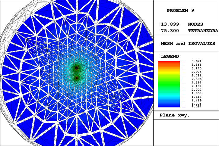
Figure 6.1: Solution to a two black hole problem.

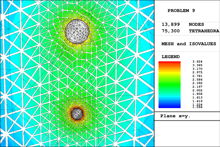
Figure 6.2: Solution to a two black hole problem, zoom.

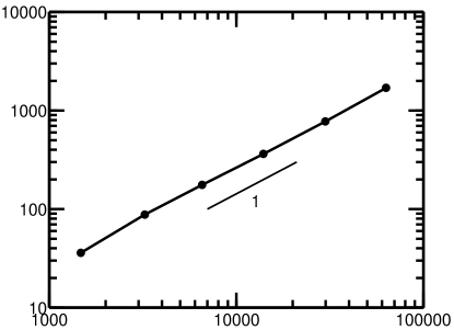
Figure 6.3: CPU seconds, on the $y$-axis, versus number of degrees of freedom, on the $x$-axis, for a binary black hole problem.

Acknowledgement
The work of the first author was supported by NSF grant DMS-9500672. The work of the third author was supported by the Swiss National Research Foundation.

Douglas N. Arnold
Department of Mathematics
Penn State University
University Park, PA 16802
USA
Arup Mukherjee
Department of Mathematics
Rutgers University
New Brunswick, NJ 08903
USA
Luc Pouly
ELCA Informatique SA
CH-1000 Lausanne
Switzerland

References

-
[1]
D. N. Arnold, A. Mukherjee, and L. Pouly,
“Locally adapted tetrahedral meshes using bisection,” Submitted
to SIAM J. Sci. Comp. (1997).
(available at http://www.math.psu.edu/dna/publications.html) - [2] E. Bänsch, “Local mesh refinement in 2 and 3 dimensions,” Impact of Comp. in Sci. and Engrg. 3 181–191 (1991).
- [3] J. Bey, “Tetrahedral grid refinement,” Computing 55, 271–288, 1995.
- [4] J. M. Bowen and J. W. York, “Time-symmetric initial data for black holes and black-hole collisions,” Phys. Rev. D 21, 2047–2056 (1980).
- [5] G. B. Cook, “Initial data for the two-body problem of general relativity,” Ph.D. Thesis, University of North Carolina at Chapel Hill (1990).
- [6] A. D. Kulkarni, “Time-asymmetric initial data for the N black hole problem in general relativity,” J. Math. Phys. 25(4), 1028–1034 (1984).
- [7] A. Liu and B. Joe, “On the shape of tetrahedra from bisection,” Math. Comp. 63(207) 141–154 (1994).
- [8] A. D. Kulkarni and L. C. Shepley and J. W. York, “Initial data for N black holes,” Phys. Lett. 96A(5) 228–230 (1983).
- [9] J. M. Maubach, “Local bisection refinement for n-simplicial grids generated by reflection,” SIAM J. Sci. Comput. 16(1) 210–227 (1995).
- [10] J. M. Maubach, “The amount of similarity classes created by local -simplicial bisection refinement,” preprint (1997).
-
[11]
A. Mukherjee, “An adaptive finite element code for elliptic boundary
value problems in three dimensions with applications in numerical relativity,”
Ph.D. Thesis, Penn State University (1996).
(available at http://www.math.psu.edu/dna/publications.html) - [12] M. C. Rivara, “Local modification of meshes for adaptive and/or multigrid finite-element methods,” J. Comput. Appl. Math. 36 79–89 (1991).
- [13] M. C. Rivara and C. Levin, “A 3-D refinement algorithm suitable for adaptive and multi-grid techniques,” Comm. in App. Num. Meth. 8 218–290 (1992).
- [14] J. W. York,“ Conformally invariant orthogonal decomposition of symmetric tensors on Riemanian manifolds and the initial-value problem of general relativity,” J. Math. Phys. 14 456–464 (1973).
- [15] J. W. York and T. Piran, “The initial value problem and beyond.” In: Spacetime and Geometry: The Alfred Schild Lectures, R. Matzner and L. Shepley eds., University of Texas Press, Austin, 1982.