Topological Black Holes – Outside Looking In

Abstract

I describe the general mathematical construction and physical picture of topological black holes, which are black holes whose event horizons are surfaces of non-trivial topology. The construction is carried out in an arbitrary number of dimensions, and includes all known special cases which have appeared before in the literature. I describe the basic features of massive charged topological black holes in $(3+1)$ dimensions, from both an exterior and interior point of view. To investigate their interiors, it is necessary to understand the radiative falloff behaviour of a given massless field at late times in the background of a topological black hole. I describe the results of a numerical investigation of such behaviour for a conformally coupled scalar field. Significant differences emerge between spherical and higher genus topologies.

1 Introduction

It has become clear over the last decade that black holes have an essential role to play in the development of a quantum theory of gravity. Each aspect of the physics of black holes – their formation due to gravitational collapse, their interior structure after formation, their thermodynamic properties, the singularities cloaked by their event horizons, and the endpoint of their evolution after thermally evaporating – present a set of interconnected puzzles whose ultimate resolution presumably entails the development of a full theory of quantum gravity. The most promising developments along this line have been in terms of the string-theoretic and Ashtekar proposals for quantum gravity, although a number of other candidate ideas exist, including non-commutative geometries, gauge-theoretic formulations, quantization of topologies, gravity as an induced phenonemon, and so on. These ideas are not mutually exclusive, and it is conceivable that the full theory of quantum gravity could contain some elements of each. Despite enormous effort, however, a full theory of quantum gravity remains elusive.

However the efforts expended towards achieving such a theory have yielded a large and still growing panoply of black objects, including black holes, black strings, and black branes. In general a spacetime containing a black object is one which has at least one event horizon: a surface which bounds a region of spacetime that is causally cut off from future timelike infinity. This surface is a null surface beyond which light (and hence all other forms of mass-energy) cannot escape. Each black object presents us with a theoretical laboratory in which we can test some of our basic ideas about the fundamental nature of gravity and its interactions with other forms of mass-energy.

One of the more interesting black objects to have entered the scene in recent times arose from the realization that certain identifications in anti-de Sitter spacetime in $(2+1)$ dimensions yields a spacetime which can be interpreted as a black hole of definite mass $M$ and angular momentum $J$ in a spacetime with cosmological constant $\Lambda=-1/\ell^{2}$. The construction was originally given by Bañados, Teitelboim and Zanelli [1] and is generally referred to as the BTZ black hole. Although originally presented as a formal, mathematical construction [1, 2], it was quickly realized that these black holes can ‘physically’ form from the collapse of $(2+1)$-dimensional matter [3] and indeed have many features in common with their more conventional $(3+1)$-dimensional counterparts [4].

Since the exterior spacetime of a collapsing $(2+1)$ dimensional black hole is locally anti-de Sitter, its singularity structure differs considerably from that of its Schwarzchild anti-de Sitter counterpart in $(3+1)$ dimensions. The Kretschmann scalar ${\cal K}=R_{\mu\nu\alpha\beta}R^{\mu\nu\alpha\beta}$ has a power-law divergence at the origin in the latter case, whereas for the BTZ black hole it is everywhere finite. Instead the BTZ black hole has a causal singularity, which occurs where the identifications surfaces merge in $(2+1)$ dimensional anti-de Sitter spacetime. These properties suggest that a study of its interior structure along the lines of that carried out for mass inflation of $(3+1)$ dimensional Reissner-Nordstrom-Vaidja black holes [5] would be interesting. Such a study was carried out by Chan et. al. for the rotating BTZ-Vaidya black hole [6] and yielded several interesting results. Assuming the radiative falloff in the BTZ-Vaidya solution has a power-law tail, the mass function diverges at the Cauchy horizon in the interior of the black hole, but all the scalar curvature invariants remain finite, and tidal distortions remain bounded. However some higher-derivative curvature scalars diverge. This forms an interesting test [7] of the Konkowski-Helliwell conjecture, which predicts the stability of Cauchy horizons based upon the behavior of test fields, and in the case of instability also predicts the nature of the singularities produced [8]. More recently, it has been shown that the assumption of a power-law falloff for the BTZ-Vaidya black hole is not correct, and that the falloff rate is exponential [9]. This does not change any of the basic results mentioned above provided the falloff rate is sufficiently weak. However for $|\Lambda|J^{2}/M^{2}>.64$, the exponential falloff rate is so large that mass inflation is cut off.

Intriguing as these effects are, their restriction to $(2+1)$ dimensions suggests at least that a considerable amount of caution be exercised in applying them to $(3+1)$ dimensions. One way of extending these results to $(3+1)$ dimensions is to embed the BTZ solution within a $(3+1)$-dimensional dilaton theory of gravity. The resultant solution may be interpreted as a spinning black string [10] and it exhibits mass inflation effects similar to its $(2+1)$ dimensional BTZ counterpart [11].

However within the last year it has been shown that higher-dimensional generalizations of the $(2+1)$-dimensional BTZ construction exist. This yields an interesting new set of black holes with event horizons of non-trivial topologies. One can obtain these black holes by either constructing higher-dimensional counterparts of the identifications in anti-de Sitter spacetime [12, 13] or by systematic elimination of the conical singularities in the cosmological C-metric [14].

In this article I shall describe the basic properties of these topological black holes from both an exterior and an interior viewpoint. I shall first describe their basic construction in terms of identifications on anti-de Sitter spacetime. I shall then move on to outline some of their basic properties, and discuss how they can form from a distribution of collapsing dust. I shall then explore the behaviour of the radiative falloff of waves outside these black hole, a necessary precursor to obtaining a more detailed understanding of their interior structure. Finally, I shall close with a discussion of the possible relevance of topological black holes to physics and of some recent research into this subject.

2 Describing Topological Black Holes

Topological black holes may be constructed by beginning with anti-de Sitter spacetime and then judiciously imposing certain identifications which have the effect of generating event horizons in the resultant quotient spacetime, thereby yielding a black hole. The treatment given here has not appeared before in the literature, although various aspects of certain details have [12, 13, 14].

Start with $(n+1)$ dimensional anti-de Sitter spacetime. This can be described by a hypersurface in an $(n+2)$-dimensional flat space of signature $(n-2,2)$

$$ds^{2}=-dx^{2}_{0}+dx^{2}_{1}+\cdots+dx^{2}_{m-1}+dx^{2}_{m}+\cdots+dx^{2}_{n}-dx^{2}_{n+1}$$ (1)

where the equation of constraint for the hypersurface is

$$-x^{2}_{0}+x^{2}_{1}+\cdots+x^{2}_{m-1}+x^{2}_{m}+\cdots+x^{2}_{n}-x^{2}_{n+1}=-\ell^{2}$$ (2)

where $\ell$ is constant.

Consider next the subspace described by the coordinates $(x_{0},\ldots,x_{m})$. This $m$-dimensional Minkowski subspace has the isometry group SO(m-1,1), with the associated Killing vectors

$$J_{\alpha\beta}=-J_{\beta\alpha}=\left(x_{\alpha}\partial_{\beta}\pm x_{\beta}\partial_{\alpha}\right)$$ (3)

where $\alpha,\beta=0,\ldots,m-1$, and the plus sign is chosen if one of $\alpha$ or $\beta$ is $0$. The idea now is to identify points in this subspace which are connected by some discrete subgroup $\Gamma$ of the isometries which are generated by the $J_{\alpha\beta}$. This of course can be done in a variety of ways for the many different discrete subgroups. However most of these identifications will yield closed timelike curves (CTCs) because points in the $x_{0}$ direction will end up being identified.

Hence the identification subspaces must lie in a region where the Killing vectors are spacelike to avoid CTCs. This yields the constraint

$$x^{2}_{0}-\left(x^{2}_{1}+\cdots+x^{2}_{m-1}\right)=R^{2}>0$$ (4)

on the Minkowskian subspace coordinates. Reparametrizing the coordinates so that

$$RX_{\alpha}=\frac{R_{+}}{\ell}x_{\alpha}$$ (5)

(where $R_{+}$ is an arbitrary constant) implies that the $m$-dimensional Minkowski subspace metric may be written as

$$ds^{2}_{m} = -dx^{2}_{0}+dx^{2}_{1}+\cdots+dx^{2}_{m-1}$$ (6)

$$= \frac{\ell^{2}}{R^{2}_{+}}\left[-dR^{2}+R^{2}\left(-dX^{2}_{0}+dX^{2}_{1}+\cdots+dX^{2}_{m-1}\right)\right]$$

where

$$-X^{2}_{0}+X^{2}_{1}+\cdots+X^{2}_{m-1}=-\frac{R^{2}_{+}}{\ell^{2}}\qquad.$$ (7)

This latter constraint means that we can write the quotient subspace metric as

$$ds^{2}_{m}=-\frac{\ell^{2}}{R^{2}_{+}}dR^{2}+R^{2}d\sigma^{2}_{m-1}$$ (8)

after identification. The metric

$$d\sigma^{2}_{m-1}=\frac{\ell^{2}}{R^{2}_{+}}\left(-dX^{2}_{0}+dX^{2}_{1}+\cdots+dX^{2}_{m-1}\right)$$ (9)

with the constraint (7) describes, after identification, a compact $(m-1)$-dimensional space $\Sigma$ of negative curvature, with $\Sigma=H^{m-1}/\Gamma$.

The coordinate $R$ is timelike within the $m$-dimensional subspace, but within the full spacetime is actually timelike. The full metric may now be written as

$$ds^{2}=-\frac{\ell^{2}}{R^{2}_{+}}dR^{2}+R^{2}d\sigma^{2}_{m-1}+dx^{2}_{m}+\cdots+dx^{2}_{n}-dx^{2}_{n+1}$$ (10)

where the constraint (2) becomes

$$x^{2}_{m}+\cdots+x^{2}_{n}-x^{2}_{n+1}=\ell^{2}\left(\frac{R^{2}}{R^{2}_{+}}-1\right)\qquad.$$ (11)

From (11) is clear that the above identification procedure has broken up the original anti-de Sitter spacetime into various causal regions that are parametrized by the magnitude of $R$. When $R=R_{+}$ the coordinates $(x_{m},\ldots,x_{n+1})$ describe a null hypersurface. This will later be seen to be the event horizon of the black hole. The region $R>R_{+}$ will correspond to the exterior of the black hole, and the region $R<R_{+}$ will correspond to the black hole interior, with $R=0$ being a singular point where the identification procedure becomes degenerate, the condition (4) being violated.

To see that the metric (10) actually describes a black hole, it is helpful to reparametrize the remaining coordinates

$$\sqrt{R^{2}-R^{2}_{+}}Y_{I}=\frac{R_{+}}{\ell}x_{n+1-I}\qquad\qquad I=m,\ldots,n+1$$ (12)

in which case (11) becomes

$$Y^{2}_{1}+\cdots+Y^{2}_{n-m+1}-Y^{2}_{0}=1$$ (13)

in the region $R>R_{+}$. The orthogonal subspace metric may be written as

$$ds^{2}_{n-m+1} = dx^{2}_{m}+\cdots+dx^{2}_{n+1}$$

$$= \frac{\ell^{2}}{R^{2}_{+}}\left[\frac{R^{2}}{R^{2}-R^{2}_{+}}dR^{2}+(R^{2}-R^{2}_{+})\left(-dY^{2}_{0}+dY^{2}_{1}+\cdots+dY^{2}_{n-m+1}\right)\right]$$

in terms of the $Y$-coordinates and $R$. The metric in the spatial $Y$ coordinates may be rewritten in terms of $(n-m+1)$ dimensional spherical coordinates

$$dY^{2}_{1}+\cdots+dY^{2}_{n-m+1}=d\rho^{2}+\rho^{2}d\Omega^{2}_{n-m}$$ (15)

and the constraint (13) becomes

$$\rho^{2}-Y^{2}_{0}=1\qquad.$$ (16)

This suggests the coordinate transformation

$$\rho=\cosh\left(\frac{R_{+}}{\ell^{2}}t\right)\qquad Y_{0}=\sinh\left(\frac{R_{+}}{\ell^{2}}t\right)$$ (17)

which yields

$$ds^{2}_{n-m+1}=\frac{\ell^{2}}{R^{2}_{+}}\left[\frac{R^{2}}{R^{2}-R^{2}_{+}}dR^{2}+(R^{2}-R^{2}_{+})\left(-\frac{R^{2}_{+}}{\ell^{4}}dt^{2}+\cosh^{2}\left(\frac{R_{+}}{\ell^{2}}t\right)d\Omega^{2}_{n-m}\right)\right]$$ (18)

for the orthogonal subspace metric.

Inserting (18) into (10) yields the final result

$$ds^{2}=\frac{\ell^{4}}{R^{2}_{+}}N(R)\left(-\frac{R^{2}_{+}}{\ell^{4}}dt^{2}+\cosh^{2}\left(\frac{R_{+}}{\ell^{2}}t\right)d\Omega^{2}_{n-m}\right)+\frac{dR^{2}}{N(R)}+R^{2}d\sigma^{2}_{m-1}$$ (19)

which is the general metric for an $(n+1)$-dimensional topological black hole. The function $N(R)$ is given by

$$N(R)=\frac{R^{2}-R^{2}_{+}}{\ell^{2}}$$ (20)

and plays the role of a generalized lapse function in the metric (19).

The metric (19) is an exact solution to the Einstein equations with negative cosmological constant in $(n+1)$ dimensions. The event horizon at $R=R_{+}$ is the direct product of null $(n-m)$-sphere with $\Sigma$, a generalization of the usual event horizon of a spherically symmetric black hole in $(3+1)$ dimensions which is a direct product of a pair of crossed null lines (i.e. a null $0$-sphere) with a $2$-sphere. Similarly, using (4), (10), and (11), one can see that there is a singularity at $R=0$ which is the direct product of a hyperbolic surface with $\Sigma$, generalizing the usual singularity which is the direct product of a hyperbola with a $2$-sphere.

It is easier to appreciate some of the features of this metric by considering a few special cases.

• $m=n=2\quad$ The metric is

  $$ds^{2}=-N(R)dt^{2}+\frac{dR^{2}}{N(R)}+R^{2}d\phi^{2}$$ (21)

  which is the static BTZ metric. The compact space $\Sigma$ is a circle. The event horizon is the direct product of a pair of crossed null lines with this circle, and the singularity at $R=0$ is the direct product of a hyperbola with this circle.

• $m=n=3\quad$ The metric is now

  $$ds^{2}=-N(R)dt^{2}+\frac{dR^{2}}{N(R)}+R^{2}\left(d\theta^{2}+\sinh^{2}(\theta)d\phi^{2}\right)$$ (22)

  which are the $(3+1)$ dimensional topological black holes discussed in refs. [12, 14]. The space $\Sigma=\Sigma_{g}$ is a Riemann 2-surface of genus $g$. The event horizon is the direct product of a pair of crossed null lines with $\Sigma_{g}$ and the singularity at $R=0$ is the direct product of a hyperbola with $\Sigma_{g}$.

  The compactness of $\Sigma_{g}$ can be understood in the following way. The coordinates $(\theta,\phi)$ are the coordinates of a hyperbolic space or pseudosphere. Geodesics on the pseudosphere are formed from intersections of the psuedosphere with planes through the origin, and are the analogs of great circles on a surface of constant positive curvature (a sphere), which are intersections of the sphere and planes through the origin. A projection of the psuedosphere onto the $(y_{1},y_{2})$ plane is known as a the Poincaré disk. On it, geodesics are segments of circles, orthogonal to the disk boundary at the edges. The pseudosphere, its associated Poincaré disk and the geodesics are shown in figure 1.

  Figure 1: The pseudosphere is one half of the hyperboloid. Beneath the pseudosphere is the Poincaré disk, the center of which is the origin.

  Consider a polygon centered at the origin of the pseudosphere whose sides are geodesics. By identifying opposite sides of this polygon a compact surface on the pseudosphere can be obtained. The angles of the polygon must sum to $2\pi$ or more, and the number of sides must be a multiple of four in order to avoid conical singularities [15]. Since the geodesics on the pseudosphere meet at angles smaller than those for geodesics meeting on a flat plane, an octagon is the simplest solution, yielding a surface of genus 2. This construction is shown in figure 2. In general, a polygon of $4g$ sides yields a surface of genus $g$, where $g\geq 2$.

  Figure 2: The identification of the octagon is shown. Opposite sides of the octagon are identified as in 2A, with sides drawn straight for clarity. Dashed lines indicate where sides have been sewn together. Sides $1$ and $1^{\prime}$ are first identified, folding the top and bottom of the octagon away from view (2B). The sides $2$ and $2^{\prime}$ are then brought together to form a torus with a diamond shaped hole, as in 2C. Next, sides $3$ and $3^{\prime}$ are stretched out and joined in 2D. The loop is lengthened along the direction of identification 3 and bent until $4$ and $4^{\prime}$ meet, forming a second torus. Finally the topology is deformed to the preferred shape, seen in 2F. Identification of a polygon of $4g$ sides will result in $g$ attached tori or, equivalently, a $g$-holed pacifier.

• $m=2,n=3\quad$ The metric is

  $$ds^{2}=N(R)\left(-dt^{2}+\frac{\ell^{4}}{R^{2}_{+}}\cosh^{2}\left(\frac{R_{+}}{\ell^{2}}t\right)d\theta^{2}\right)+\frac{dR^{2}}{N(R)}+R^{2}d\phi^{2}$$ (23)

  which describes the metric of an alternate generalization of the BTZ black hole discussed recently by Holst and Peldan [16]. The coordinate $\theta$ is periodically identified. The compact space $\Sigma$ is again a circle with coordinate $\phi$. The event horizon is the direct product of a null conoid (i.e. a null circle) with this circle, and the singularity is the direct product of a 2-dimensional hyperboloid with this circle.

  Under the coordinate transformation

  $$\sinh(\frac{R_{+}t}{\ell^{2}})=\cosh(T/\ell)\sqrt{X^{2}-1}\qquad\tan(\theta)=\sinh(T/\ell)\frac{\sqrt{X^{2}-1}}{X}$$ (24)

  the $(t,\theta)$ section transforms as

  $$-dt^{2}+\frac{\ell^{4}}{R^{2}_{+}}\cosh^{2}\left(\frac{R_{+}}{\ell^{2}}t\right)d\theta^{2}=\frac{\ell^{4}}{R^{2}_{+}}\left(-\frac{dX^{2}}{X^{2}-1}+(X^{2}-1)dT^{2}/\ell^{2}\right)$$ (25)

  where the coordinate transformation is valid provided $|X|>1$. It is clear from (25) that these coordinates can be extended to the $|X|\leq 1$ region, in which $X$ becomes a spatial coordinate and $T$ becomes a timelike coordinate. Writing $X=\cos\lambda$ yields

  $$\frac{\ell^{4}}{R^{2}_{+}}\left(-\frac{dX^{2}}{X^{2}-1}+(X^{2}-1)dT^{2}/\ell^{2}\right)=\frac{\ell^{4}}{R^{2}_{+}}\left(d\lambda^{2}-\sin^{2}\lambda\ dT^{2}/\ell^{2}\right)$$ (26)

  which implies that

  $$ds^{2}=N(R)\frac{\ell^{4}}{R^{2}_{+}}\left(d\lambda^{2}-\sin^{2}\lambda\ dT^{2}/\ell^{2}\right)+\frac{dR^{2}}{N(R)}+R^{2}d\phi^{2}$$ (27)

  which is also a solution to the Einstein equations with negative cosmological constant.

  The metric (27) is the constant curvature black hole (CCBH) discussed earlier [13]. Its global properties differ from those of the metric (23) in that the event horizon is the direct product of a pair of null conoids joined at their apexes with the circle $\Sigma$. Note that $\partial/\partial T$ is a Killing vector of the metric (27), but that $\partial/\partial t$ is not a Killing vector of the metric (23). In this sense the event horizon of (23) evolves with respect to the time coordinate $t$ [16].

3 Properties of Topological Black Holes

I shall consider only $(3+1)$ dimensional black holes throughout the sequel. For the solutions (22) it is possible to add mass and charge [14], yielding

$$ds^{2} = -\left(R^{2}/l^{2}-1-2m/R+q^{2}/R^{2}\right)dt^{2}+\frac{dR^{2}}{R^{2}/l^{2}-1-2m/R+q^{2}/R^{2}}$$ (28)

$$\qquad+R^{2}\left(d\theta^{2}+\sinh^{2}(\theta)d\phi^{2}\right)$$

which is an exact solution of the Einstein-Maxwell equations with negative cosmological constant $\Lambda=-3/\ell^{2}$. The metric for fixed $(t,R)$ is assumed to be identified in the $(\theta,\phi)$ coordinates as decribed previously, so that it describes a black hole whose event horizon is of genus $g\geq 2$. The electromagnetic field strength is

$$F=-\frac{q}{R^{2}}dt\wedge dR$$ (29)

in the electric case, and

$$F=q\sinh\theta d\theta\wedge d\phi$$ (30)

in the magnetic case. Toroidal black holes (genus $g=1$) have the metric

$$ds^{2}=-\left(R^{2}/l^{2}-2m/R+q^{2}/R^{2}\right)dt^{2}+\frac{dR^{2}}{R^{2}/l^{2}-2m/R+q^{2}/R^{2}}$$

$$+R^{2}\left(d\theta^{2}+d\phi^{2}\right)$$ (31)

with

$$F=-\frac{q}{R^{2}}dt\wedge dR\qquad F=qd\theta\wedge d\phi$$ (32)

in the electric and magnetic cases respectively, where $\theta$ and $\phi$ are periodically identified. Note that the entire spacetime has topology $R^{2}\times H^{2}_{g}$ for a genus $g\geq 1$ black hole.

Using the quasilocal formalism developed for anti de Sitter spacetimes [17] it is straightforward to show that

$$M=m(|g-1|+\delta_{g,1})$$ (33)

is the conserved mass parameter associated with the Killing vector $\partial/\partial t$. for genus $g\geq 1$ [18, 19]. Similarly,

$$Q=q(|g-1|+\delta_{g,1})$$ (34)

is the conserved charge $Q$ associated with a genus $g$ black hole.

The genus $g$ metric function

$$V(r)\equiv R^{2}/l^{2}-(1-\delta_{g,1}-2\delta_{g,0})-2m/R+q^{2}/R^{2}$$ (35)

has at most two roots for positive $R$, corresponding to an inner and outer horizon, as with the usual $g=0$ Reissner-Nordstrom anti de Sitter metric. For $g=1$, provided

$$27\,l^{2}\,{\it m}^{4}\geq 16\,q^{6}$$ (36)

there are two horizons, with the extremal case saturating the inequality. For $g\geq 2$ event horizons exist provided

$$m^{2}\leq{\displaystyle\frac{l^{2}}{27}}\,{\displaystyle\frac{16-24\,e^{2}b-16b\sqrt{1-e^{2}b}\,e^{2}+6b^{2}\,e^{4}+16\,\sqrt{1-e^{2}b}}{e^{6}}}$$ (37)

where $e=\frac{2\sqrt{2}q}{3m}$. There is no (obvious) upper limit on e, and event horizons can exist for arbitrarily large values of $q$ relative to $m$.

The causal structure of these spacetimes is similar to that of Reissner-Nordstrom anti de Sitter spacetime with spherical topology. The three causal diagrams in the neutral, sub-extremal and extremal cases are shown in Fig. 3. A curious feature of these higher-genus black holes is that the mass parameter need not be positive in order for an event horizon to exist [20], even if the black hole is uncharged.

Figure 3: Causal diagrams for topological black holes in the neutral, subextremal and extremal cases. The subextremal case can be that of a charged black hole or of a negative mass black hole.

An extensive study of the thermodynamic properties of these black holes was recently carried out by Brill et. al. [19]. The entropy/area relation

$$S=\frac{1}{4}A$$ (38)

was found to hold, although this result has been disputed by Vanzo [21]. Their heat capacities $C_{X}=T\left(\frac{\partial S}{\partial T}\right)_{X}$ were also computed, and found to be of indefinite sign if $g\geq 2$.

It has also been demonstrated that topological black holes of arbitrary genus can form from the gravitational collapse of pressureless dust [22]. Although the procedure is somewhat analogous to that in the spherical case, there are a few interesting discrepancies. For non-trivial topologies, collapse from rest will not take place unless

$$\Lambda>8\pi G\rho_{0},$$ (39)

where $\rho_{0}$ is the initial density of the cloud. A more general but qualitatively similar condition holds if the dust cloud is given some initial velocity. The exterior spacetime formed is that given by (28) with $q=0$. Another interesting feature is that collapse can take place even for dust which violates the weak energy condition, i.e. $\rho_{0}<0$. Provided the initial negative energy density is not too large in magnitude, a cloud of negative energy dust can collapse to a topological black hole of negative mass [20].

Finally, topological black holes may be pair produced in the presence of a domain wall of suitable topology [14, 18]. The mechanism is analogous to that discussed for other cosmological black holes [23, 24].

4 Inside Topological Black Holes?

Both charged and negative mass topological black holes have inner as well as outer event horizons. As can be seen from figure 3, the maximal extensions of such black hole spacetimes can be imagined as a collection of different asymptotically anti de Sitter universes connected by different charged (or negative mass) black holes. The presence of the inner horizon causes any radiation (either scalar, electromagnetic or gravitational in nature) entering this kind of black hole to be indefinitely blue-shifted at the inner (or Cauchy) horizon.

Does the phenomenon of mass inflation [25] take place for topological black holes? There are in general three necessary ingredients for mass inflation to take place: the existence of a Cauchy horizon, the presence of radiation which enters the black hole at some rate which decays at late times, and the possibility of cross-flow of this radiation with that emitted from a collapsing object that is forming the black hole. The first condition is clearly satisfied by either charged or negative mass black holes. Since both kinds of black holes can be formed from gravitational collapse, it is clear that the third condition can be satisfied provided the second one is.

An understanding of the nature of radiative falloff outside topological black holes is therefore crucial insofar as investigating their interior is concerned. For asymptotically flat spacetimes, the radiative falloff at late times obeys a power-law [26]. However this situation changes for other kinds of spacetimes. For example Mellor and Moss have shown that the radiation from perturbations in a de Sitter background exponentially decreases [27]. Strictly speaking this result has nothing to do with late time falloff since the global geometry extends beyond the cosmological horizon. However it does indicate that the radiative falloff behaviour is sensitive to the asymptotic structure of the spacetime. Indeed, for conditions more general that simple asymptotic flatness, the tail can be something other than an inverse power-law [28].

A recent investigation [29] of radiative falloff in Schwarzchild anti de Sitter spacetime indicated that the late time falloff behaviour is considerably more complicated than that in either asymptotically flat or asymptotically de Sitter spacetimes. This is a consequence of spatial infinity being timelike – although the proper distance to any point at large $R$ in such a spacetime diverges as $R\to\infty$, a light ray can travel to arbitrarily large $R$ in a finite amount of time.

A useful means for probing the falloff behaviour of late times is to study the conformally coupled scalar wave equation. The scalar wave equation has qualitatively the same behaviour and its more complicated electromagnetic and gravitational tensorial counterparts, and the conformal coupling ensures that the effective potential in which the wave moves most closely resembles the previously studied asymptotically flat case [29].

The (conformally coupled) scalar wave equation in $(3+1)$ dimensions is

$$\nabla^{2}\Psi = \xi\,R\,\Psi\;,$$ (40)

where $\xi$ is an arbitrary constant. If $\xi=\frac{1}{6}$ this equation is conformally invariant. The form of the metric for topological black holes is

$$ds^{2} = \mbox{-}\,V(r)\,dt^{2}+\frac{dr^{2}}{V(r)}+r^{2}\,d{\Omega_{g}}^{2}\;,$$ (41)

where $V(r)$ is the lapse function given by (35) and $d{\Omega_{g}}^{2}$ is the metric of a genus $g$ Riemann surface. Assuming the separability condition

$$\Psi = \frac{1}{r}\,\psi(t,r)\,{\cal Y}(\Omega_{g})_{l}$$ (42)

it is straightforward to show that equation (40) gives

$$\mbox{-}\,\partial_{tt}\psi(t,r)+V(r)\,\partial_{r}\left[\,N(r)\,\partial_{r}\psi(t,r)\,\right]-V(r)\,V_{e}(r)\,\psi(t,r) = 0$$ (43)

where

$$V_{e}(r) \equiv \xi\,R+\frac{1}{r}\,\frac{d}{d\,r}V(r)+\frac{l(l+1)}{r^{2}}$$ (44)

defines the function $V_{e}(r)$. The functions ${\cal Y}_{l}$ are the genus $g$ analogues of the spherical harmonics [15], and for $g\geq 2$, say, satisfy the equation

$$\hat{L}^{2}\!\left[\,{\cal Y}_{l}\,\right]\equiv\left[\frac{1}{\sinh\theta}\frac{\partial}{\partial\theta}\left(\sinh\theta\frac{\partial}{\partial\theta}\right)+\frac{1}{\sinh^{2}\theta}\frac{\partial^{2}}{\partial\phi^{2}}\right]{\cal Y}_{l}=\mbox{-}\,l\,(l+1)\,{\cal Y}_{l}$$ (45)

and are referred to as conical functions.

For simplicity the scalar wave will be assumed to be independent of $(\theta,\phi)$. One can then rewrite the wave equation (43) as

$$\partial_{tt}\psi\!\left(\,t,r(x)\,\right)-\partial_{xx}\psi\!\left(\,t,r(x)\,\right)+{\cal V}\!\left(\,r(x)\,\right)\,\psi\!\left(\,t,r(x)\,\right) = 0$$ (46)

where ${\cal V}(x)\equiv V(r(x))V_{e}(R(x))$ with $l=0$ and

$$x\;\equiv\;\int\frac{dr}{N(r)}$$ (47)

is the so-called tortoise coordinate.

The function ${\cal V}(r)$ plays the role of a potential barrier which is induced from the background spacetime geometry. Equation (46) has the familiar form of a potential scattering problem, although ${\cal V}$ has a rather complicated dependence on the tortoise co-ordinate $x$. It can be integrated numerically in a straightforward fashion by using finite difference methods. The D’Alembert operator $\partial_{tt}-\partial_{xx}$ is first discretized as

$$\frac{\psi(t-\Delta t,x)-2\,\psi(t,x)+\psi(t+\Delta t,x)}{{\Delta t}^{2}}\qquad$$ (48)

$$\qquad-\frac{\psi(t,x-\Delta x)-2\,\psi(t,x)+\psi(t,x+\Delta x)}{{\Delta x}^{2}} + O({\Delta t}^{2})+O({\Delta x}^{2})$$

using Taylor’s theorem. In order to formulate a well-posed Cauchy problem initial conditions must be chosen. For simplicity these can be taken to be

$$\psi(t=0,x)\;=\;0\hskip 28.45274pt {\rm and} \hskip 28.45274pt\partial_{t}\psi(t=0,x)\;=\;u(x)\;.$$ (49)

Because the field $\psi$ is initially zero, its subsequent evolution is solely the result of the initial impulse of the field $\partial_{t}\psi$. Discretizing the second condition in (49) yields

$$\frac{\psi(\Delta t,x)-\psi(\mbox{-}\,\Delta t,x)}{2\,\Delta t} = u(x)+O({\Delta t}^{2})\;,$$ (50)

where a Gaussian distribution with finite support for $u(x)$ is employed. Defining

$$\psi(m\,\Delta t,n\,\Delta x) \equiv \psi_{m,n}\;,$$ (51)

$$V(n\,\Delta x) \equiv V_{n}\;,$$ (52)

$$u(n\,\Delta x) \equiv u_{n}\;,$$ (53)

where the mesh size has to satisfy the condition $\Delta x>\Delta t$ so that the numerical rate of propagation of data is greater than its analytical counterpart.

If the black hole geometry is asymptotically flat, the tortoise coordinate $x$ goes from negative infinity to positive infinity. When the background is asymptotically anti de Sitter the initial data no longer enjoy this privilege because the tortoise coordinate goes from minus infinity to zero only. In other words, rightward propagating data cannot travel in this direction forever. As with the semi-infinite vibrating string problem, boundary conditions at spatial infinity (i.e. $x=0$) are needed in the asymptotically anti de Sitter background in order to formulate the problem appropriately. Here the boundary conditions employed will be either

$$\psi(t,x=0)\;=\;0\hskip 28.45274pt {\rm and} \hskip 28.45274pt\partial_{x}\psi(t,x=0)\;=\;1$$ (54)

which are referred to as the Dirichlet boundary conditions, or

$$\psi(t,x=0)\;=\;1\hskip 28.45274pt {\rm and} \hskip 28.45274pt\partial_{x}\psi(t,x=0)\;=\;0\;.$$ (55)

which are the Neumann boundary conditions.

Both of these boundary conditions will be used in investigated the radiative falloff of conformally coupled waves in the topological black hole spacetimes (41). For simplicity, only neutral topological black hole spacetimes will be considered.

5 Radiative Falloff Outside Neutral Topological Black Holes

Before presenting the results of the numerical analysis of equation 46 it will be worthwhile recapitulating what takes place in Schwarzchild and Schwarzchild anti de Sitter spacetimes [29]. The wave equation (46) in all cases is solved numerically using the scheme discussed in the previous section, and $\xi=\frac{1}{6}$ throughout.

Figure 4 shows the general form of the potential ${\cal V}(x)$ for a background Schwarzschild spacetime in both linear and logarithmic coordinates (with the $l=1$ spherical harmonic). The bottom diagram in 4 is a logarithmic plot of the magnitude of the scalar wave at the point $RO=20M$ as a function of time, where the compact initial Gaussian pulse is at the point $Ro=10M$ (or $x=12.76\,M$). The field vanishes until the pulse has propagated outwards to the point $RO$. It reaches its maximum value, after which it undergoes a “ringing” effect due to the presence of quasinormal modes [28]. This ringing dies out after $t\approx 200$, after which the field decays according to a smooth power law which from linear regression, is found to have a slope of $\mbox{-}\,5.026$ in agreement with the analytic prediction of an inverse power-law falloff with exponent $2\,l+3$ [26].

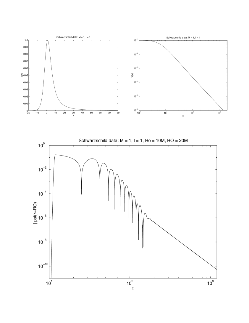
Figure 4: The potential ${\cal V}(x)$ in a Schwarzschild background and the resultant decay of a scalar wave. Prior to $t\approx 200$ the decay is accompanied by ‘ringing’ of the quasi-normal modes, after which the falloff rate is that of an inverse power-law.

The situation for Schwarzchild anti de Sitter (SAdS) spacetime is somewhat different, and is shown in figure 5. As with the Schwarzschild black hole (figure 4), the potential function $V(x)$ attains a maximum not far away from the event horizon $Rb$, given by the largest positive solution to $V(R_{b})=0$. However unlike the Schwarzschild case, the tortoise coordinate $x$ for the SAdS background is bounded above. The top part of figure 5 illustrates the shape of the potential function ${\cal V}(x)$ for a variety of values of $|\Lambda|=3/\ell^{2}$ and the spherical harmonic parameter $l$.

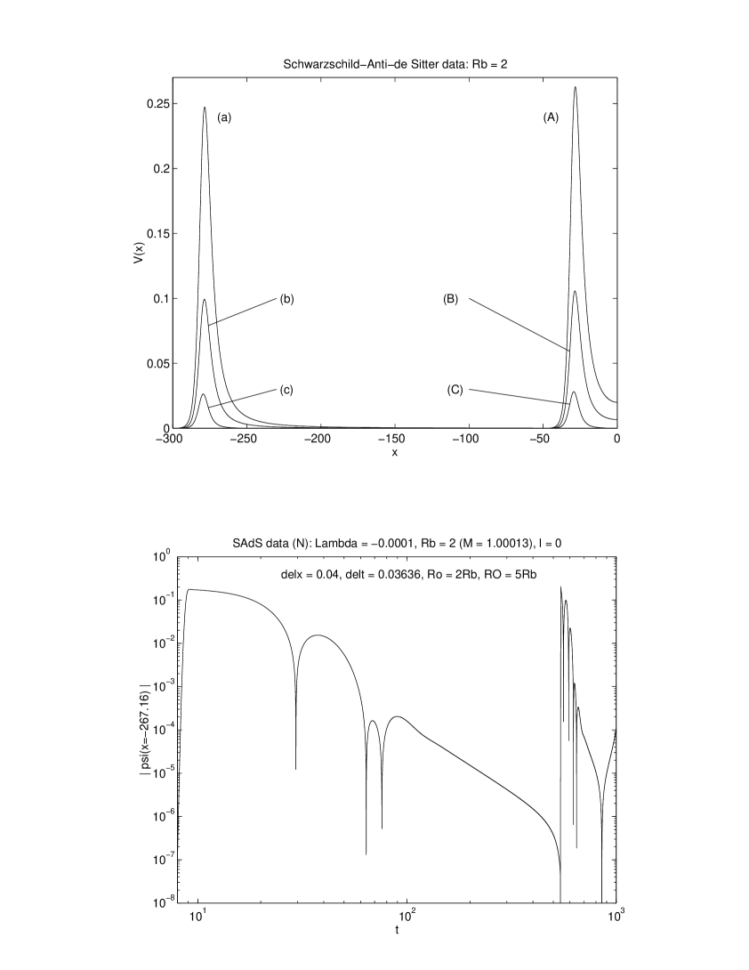
Figure 5: Potential functions $V(x)$ for the SAdS background. The six potentials are generated with the parameters (a) $\Lambda=\mbox{-}\,10^{\mbox{-}\,4},l=2$, (b) $\Lambda=\mbox{-}\,10^{\mbox{-}\,4},l=1$, (c) $\Lambda=\mbox{-}\,10^{\mbox{-}\,4},l=0$, (A) $\Lambda=\mbox{-}\,10^{\mbox{-}\,2},l=2$, (B) $\Lambda=\mbox{-}\,10^{\mbox{-}\,2},l=1$, (C) $\Lambda=\mbox{-}\,10^{\mbox{-}\,2},l=0$. The bottom diagram shows the $l=0$ scalar wave falloff pattern using Neumann condition.

Eventually all the outgoing conformal waves that leave the black hole region will return towards it due to the boundary condition at $x=0$. The returning wave will then reflect off of the potential barrier back toward spatial infinity for both the Dirichlet and Neumann boundary conditions. In this and all subsequent diagrams the quantities “delx” and “delt” on the graphs refer to the step sizes $\Delta x$ and $\Delta t$ of the variables x and t respectively, where $\Delta x>\Delta t$ holds as noted above.

For small $|\Lambda|$ and small times, the falloff behaviour resembles the Schwarzchild case. Initially there is a ringing effect (due to the quasi-normal modes) followed by inverse power-decay behaviour. However this inverse power-decay does not last very long because of the return of the outgoing wave from spatial infinity. As $l$ gets larger the ringing increases in frequency as shown in figure 6.

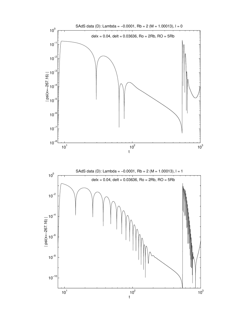
Figure 6: The $l=0$ (top) and $l=1$ (bottom) scalar wave falloff patterns using the Dirichlet condition.

As $|\Lambda|$ increases, the transient power-law effect is eliminated entirely and new behaviour emerges. For small $l$ there can be a pure ringing effect within an exponentially decaying envelope, as shown in the top part of figure 7. As $l$ increases, the ringing itself undergoes a complicated oscillation effect which mildly decays, as shown in the bottom part of figure 7.

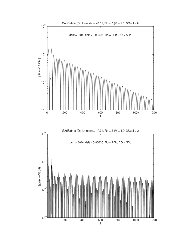
Figure 7: The $l=0$ (top) and $l=2$ (bottom) scalar wave falloff patterns using for large $|\Lambda|$.

These results are all largely insensitive to the use of either Dirichlet or Neumann boundary conditions [29].

Turning next to the (neutral) topological black hole (TBH) case, figure 8 compares the potential ${\cal V}(x)$ for $l=0$ for the SAdS (top) and TBH (bottom) cases. The event horizon is at $x=-\infty$, and spatial infinity is at $x=0$. Each potential has a maximum at some finite $x$ and decays exponentially toward the horizon. However the TBH potential does not have a point of inflection on the rightward side of the maximum, unlike the SAdS case.

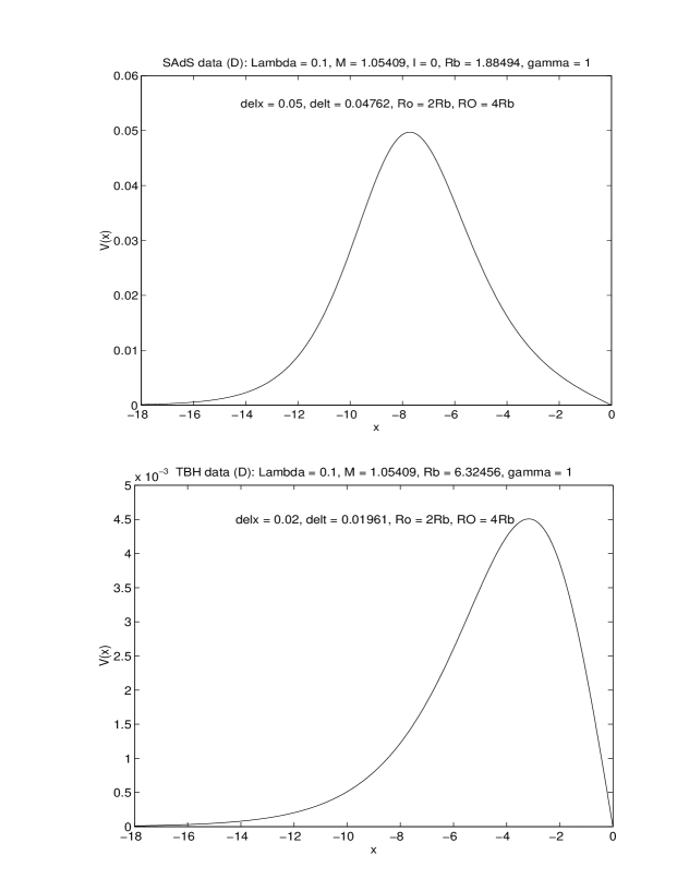
Figure 8: A comparison of the potential ${\cal V}(x)$ for the SAdS (top) and TBH (bottom) cases.

Note that even if $M$ and $\Lambda$ for a given topological black hole are equal to that of a given SAdS black hole, the location of the event horizons $Rb$ will differ because $V$[TBH] = $V$[SAdS]$-2$. One is then faced with the problem of how to meaningfully compare the falloff behaviour of a given TBH with that of a “similar” SAdS black hole for differing values of $M$ and $\Lambda$. This can be overcome by choosing to compare the SAdS and TBH cases for equal values of the parameter $\gamma\equiv 3\sqrt{3}M/\ell=3M\sqrt{|\Lambda|}$, which is a dimensionless measure of the black hole mass. This parameter governs the location of the event horizon $Rb=r_{h}\ell$, where

$$r^{3}_{h}-(1-\delta_{g,1}-2\delta_{g,0})r_{h}=\frac{2}{3\sqrt{3}}\gamma$$ (56)

defines $r_{h}$, for a genus $g$ black hole. For the SAdS case ($g=0$), $0<\gamma<\infty$, whereas for the TBH case ($g\geq 2$) $-1<\gamma<\infty$ because subextremal negative mass black holes can also be included. Here only the range $0<\gamma<\infty$ will be considered. For a given value of $\gamma$, I shall compare the SAdS, TBH ($g\geq 2$) and toroidal ($g=1$) cases over a range of values of $\Lambda$.

Consider first the cases where the genus $g\geq 2$. These cases all have the same qualitative behaviour, shown in figures 9 – 11 For large $\gamma$, the behaviour of the TBH and SAdS cases is qualitatively similar over a wide range of values of $|\Lambda|$ with some quantitative differences as shown in figure 9. Each exhibits a ringing effect which falls off exponentially with time. The ringing frequency is slightly higher and the falloff rate slightly weaker in the SAdS case that in the TBH case. For each, as $|\Lambda|$ increases the ringing frequency and the falloff rate both increase.

Figure 9: Falloff rates for the SAdS (left) and TBH (right) cases for $\gamma=10$ for a range of values of $|\Lambda|$.

These differences become more pronounced as $\gamma$ decreases. From figure 10, in which $\gamma=1$, it is clear that the approximate exponential falloff rate in the TBH case increases substantially relative to the SAdS case. In addition the ringing frequency in the SAdS case rises relative to that of the TBH case, although not as dramatically as it might first appear due to the difference in scale on the $t$-axis of the plots. These effects become slightly more pronounced as $|\Lambda|$ increases.

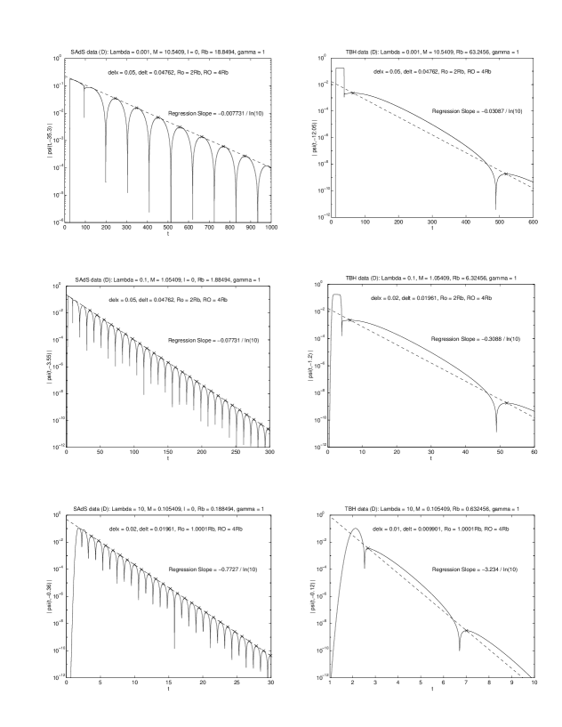
Figure 10: Falloff rates for the SAdS (left) and TBH (right) cases for $\gamma=1$ for a range of values of $|\Lambda|$.

For very small $\gamma$ substantial qualitative differences between the two cases emerge. The sequence of ringing, power-law falloff and resurgence of the wave noted above from figure 6 for the SAdS case returns. As $|\Lambda|$ increases the intermediate power-law falloff is obliterated at late times, replaced by a slowly decaying set of oscillatory ringing behaviour. However in the TBH case the ringing virtually disappears, being replaced by a smooth exponential falloff. Due to limitations in computer memory and running time, it is not possible to tell if the ringing effect has actually vanished or if the frequency is just extremely low, although the upper right graph in figure 11 would suggest that it has actually vanished. The falloff rate grows with increasing $|\Lambda|$.

Figure 11: Falloff rates for the SAdS (left) and TBH (right) cases for $\gamma=0.1$ for a range of values of $|\Lambda|$.

A comparsion of the SAdS and toroidal (genus $g=1$) cases is given in figures 12 – 14. For large $\gamma$ the toroidal case is similar to that of the genus $g\geq 2$ cases, with a slightly less rapid falloff and more frequent ringing for the toroidal case. The difference is most pronounced for small $\gamma$, with the toroidal case still exhibiting some ringing for $\gamma=0.1$. For clarity figure 15 shows a comparison at $\gamma=1$ between the higher genus (TBH) and toroidal cases.

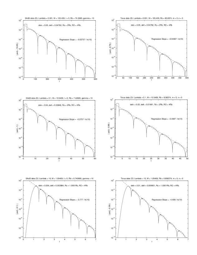
Figure 12: Falloff rates for the SAdS (left) and Toroidal (right) cases for $\gamma=10$ for a range of values of $|\Lambda|$.

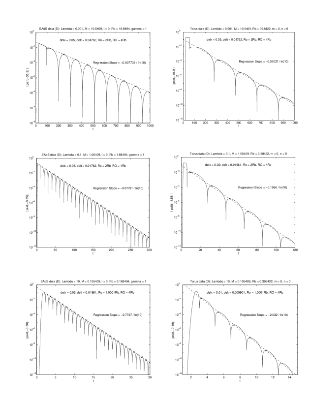
Figure 13: Falloff rates for the SAdS (left) and Toroidal (right) cases for $\gamma=1$ for a range of values of $|\Lambda|$.

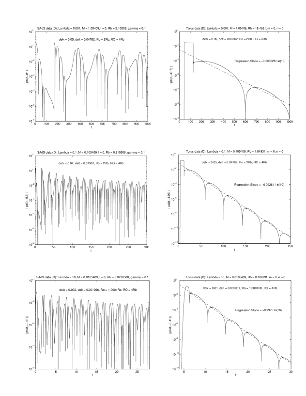
Figure 14: Falloff rates for the SAdS (left) and Toroidal (right) cases for $\gamma=0.1$ for a range of values of $|\Lambda|$.

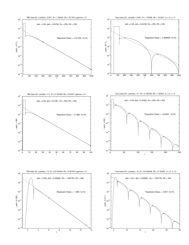
Figure 15: Falloff rates for the higher genus TBH (left) and Toroidal (right) cases for $\gamma=0.1$ for a range of values of $|\Lambda|$.

For all of the above results, the radiative falloff behaviour for topological black holes is relatively insensitive to the use of Dirichlet or Neumann boundary conditions.

6 Summary

The radiative falloff behaviour described in the previous section indicates that (charged or negative mass) topological black holes can indeed undergo mass inflation, provided the exponential falloff rate is sufficiently small. In this case the blueshift effect at the Cauchy horizon will overwhelm the exponential decay of the incoming radiation, triggering mass inflation. However it is quite conceivable that that the falloff rate could be so strong as to cut off the mass inflation process for some range of the parameter set $(\gamma,|\Lambda|)$.

Whether or not this can take place is presently under investigation. However a similar phenomenon has been observed in $(2+1)$ dimensions for the BTZ black hole. As noted above, for $|\Lambda|J^{2}/M^{2}>.64$, the exponential falloff rate outside a BTZ black hole is so large that mass inflation is cut off. A detailed study of the nature of the transition at this point is presently being carried out.

Topological black holes present us with an interesting new set of possibilites to explore in our quest to understand the physics of black holes and the role they play in quantum gravity. Although astrophysical applications of topological black holes are not immediately apparent, they will necessarily play some role in any theory of quantum gravity which includes topology changing processes.

References

- [1] M. Banados, C. Teitelboim and J. Zanelli, Phys. Rev. Lett. 69, (1992) 1849.
- [2] M. Banados, M. Henneaux, C. Teitelboim and J. Zanelli, Phys. Rev. D 48, (1993) 1506.
- [3] R.B. Mann and S.F. Ross, Phys. Rev. D47 (1993) 3319.
- [4] For a review see S. Carlip, Class. Quant. Grav. 12 (1995) 2853; for a more general review on the subject of lower dimensional black holes see R.B. Mann, Proceedings of the Winnipeg Conference on Heat Kernels and Quantum Gravity, ed. S. Christensen (Texas A& M Press, 1996) 303.
- [5] E. Poisson and W. Israel, Phys. Lett. B 233, (1989) 74 ; E. Poisson and W. Israel, Phys. Rev. D 41, (1990) 1796 .
- [6] S.F.J. Chan, K.C.K. Chan and R.B. Mann, Phys. Rev. D54 (1996) 1535.
- [7] B. Wang, R. Su and P.K.N. Yu Phys. Rev. D54 (1996) 7298.
- [8] T. M. Helliwell and D. A. Konkowski, Phys. Rev. D51, (1995) 5517; Phys. Rev. D54, (1997) 7898.
- [9] R.B. Mann and J.S.F. Chan, Phys. Rev. D55 (1997) 7546.
- [10] N. Kaloper, Phys. Rev. D48, 10, 4658 (1993).
- [11] J.S.F. Chan and R.B. Mann, Phys. Rev. D51 (1995) 5428.
- [12] S. Aminneborg, I Bengtsson, S. Holst and P. Peldan, Class. Quant. Grav. 13, (1996) 2707; D. Brill, Helv.Phys.Acta 69 (1996) 249.
- [13] M. Bañados, Report No. gr-qc/9703040 (1997).
- [14] R.B. Mann, Class. Quant. Grav. 14 (1997) L109 .
- [15] N. L. Balasz and A. Voros, Phys. Rep. 143 (1986) 109.
- [16] S. Holst and P. Peldan, Report No. gr-qc/9705007 (1997).
- [17] J.D. Brown, J. Creighton and R.B. Mann, Phys. Rev. D 50 6394 (1994).
- [18] R.B. Mann, WATPHYS-TH97/05, gr-qc/9705223.
- [19] D. Brill, J. Louko and P. Peldan, Phys. Rev. D56 (1997) 3600.
- [20] R.B. Mann, WATPHYS-TH97/03, gr-qc/9705007, to be published in Class. Quant. Grav.
- [21] L. Vanzo, UTF-400, gr-qc/9705004.
- [22] W.L. Smith and R.B. Mann, WATPHYS-TH97/02, gr-qc/9703007, to be published in Phys. Rev. D.
- [23] R.B. Mann and S.F. Ross, Phys. Rev. D52, (1995) 2254.
- [24] R.R. Caldwell, A. Chamblin and G.W. Gibbons, Phys. Rev. D53 (1996) 7103.
- [25] E. Poisson and W. Israel, Phys. Lett. B233, (1989) 74 Phys. Rev. D41, (1990) 1796.
- [26] R. H. Price, Phys. Rev. D5, (1972) 2419.
- [27] F. Mellor and I. Moss, Phys. Rev. D41, (1990) 403.
- [28] E. S. C. Ching, P. T. Leung, W. M. Suen and K. Young, Phys. Rev. D 52, (1995) 2118.
- [29] R.B. Mann and J.S.F. Chan, Phys. Rev. D55 (1997) 7546.